Composite Cluster States and Alternative Architectures for One- Way Quantum Computation
Abstract
We propose a new architecture for the measurement-based quantum computation model. The new design relies on small composite light-atom primary clusters. These are then assembled into cluster arrays using ancillary light modes and the actual computation is run on such a cellular cluster. We show how to create the primary clusters, which are Gaussian cluster states composed of both light and atomic modes. These are entangled via QND interactions and beamsplitters and the scheme is well described within the continuous-variable covariance matrix formalism.
I Introduction
The one-way model or Measurement Based Quantum Computation (MBQC) has emerged as a conceptually interesting and potentially practical alternative to the standard model of quantum computation [1]. MBQC replaces the need for coherent unitary control [2] by a sequence of adaptive local measurements performed on a highly entangled resource state known as a cluster state [3]. This resource acts as a universal substrate with quantum information encoded virtually within it. Though originally based on qubits, the cluster model has been generalized to higher dimensional discrete-variable systems (qudits) [4] as well as to continuous quantum variables [5].
In its continuous-variable (CV) incarnation, the resource state is a multimode squeezed Gaussian state. In the optical setting [6, 7], homodyne detection and photon counting plus classical feedforward, suffice to implement universal QC over CV. It has also been shown that homodyne detection alone is sufficient to implement all multimode Gaussian operations, given a cluster state with a sufficiently connected graph [8].
Many proposals for the construction of optical CV cluster states have been put forward, including the linear optical construction [6], the single optical parametric oscillator (OPO) method [9, 10] and single quantum nondemolition (QND)-gate schemes [11, 12]. These procedures are deterministic and have the advantage over their discrete counterparts [13, 14, 15], which rely on nondeterministic interactions and postselection. However, as with any CV system, these protocols suffer the usual problems such as the lack of infinitely squeezed resources leading to finite squeezing errors.
Here we will use the canonical generation method where cluster states are created from single-mode squeezers and controlled-Z () gates [5]. The controlled-Z is an example of a QND interaction and, for optical modes, can be implemented using beamsplitters and inline or offline squeezers [16, 17, 18]. This method, while experimentally challenging is achievable with current technology [19].
CV cluster states can be built, not only from optical modes but also from ensembles of polarized atoms where each ensemble is a different CV mode [20, 21, 22, 23]. The ensembles are entangled by performing interactions with off-resonant linearly polarized light, which, on the classical level, performs a Faraday rotation. The rotated light then serves as a carrier to encode information in each of the ensembles and homodyne measurements are performed to complete the protocol and project the state of the ensembles into the desired entangled state.
However, it has been shown that Gaussian cluster states suffer from a fundamental problem. Namely, no matter what Gaussian local measurements are performed on systems distributed on a general graph, transport and processing of quantum information is not possible beyond a certain influence region, except for exponentially suppressed corrections [24]. In other words, as the size of the cluster increases there is an exponential decay in the Gaussian localizable entanglement over the entire cluster which leads to the corollary that cluster states with only Gaussian operations cannot serve as perfect quantum wires. Hence large cluster states with only Gaussian resources available will always suffer from large errors.
Here we propose an architecture of a one-way computer that removes the need for large clusters. In our scheme, small, single gate-size cluster states composed of atomic ensembles are created and the computations are carried out over an array of such clusters. Due to their proven suitability as information carriers, communication between the clusters is accomplished using optical modes. The atomic ensembles we use have the advantage that they can serve as a short term quantum memory as well as a processing device due to their relatively long lived storage times. In order to get information from one processor to the next, we entangle a polarized light pulse to the ensemble. This light mode in effect becomes part of the processor cluster state. When suitable measurements are performed on the atomic modes, the information is passed onto the light. This light mode can then be coupled to the next processor and the procedure is repeated until the computation is complete. In order to realize this scheme, we require a protocol to include a light mode into an atomic cluster state. We call such a state a composite cluster state that is composed of atomic modes and light modes. Here we will explicitly demonstrate the protocol for the generation of such states.
This paper is organized as follow. In section II we will review the types of interaction we will be using and show how the two-mode composite cluster state is constructed. In section III, we discuss the protocol in the covariance matrix formalism. In section IV we discuss the entanglement properties of the state. In section V we generalize our discussion to multipartite entanglement and show how to create composite cluster states of arbitrary size. In section VI we discuss an alternative computational architecture for CV MBQC, making use of the multi-mode composite cluster states. We conclude in section VII.
II Quantum non-demolition interactions
The physical systems of interest to us are atomic ensembles and light beams. The light beams are used both as part of the required cluster state and information carriers between nodes of the cluster.
Each atomic ensemble contains a large number, , of non- interacting alkali atoms with individual total angular momentum [25]. The ensemble is described by its collective angular momentum , where
| (1) |
All atoms are assumed to be polarized along the -direction, which corresponds to preparing them in a particular hyperfine state, . Then, fluctuations in the component of collective spin are kept extremely small relative to the strong coherent excitation and we can just treat as a classical quantity, . The orthogonal components of spin are unaffected by the -polarization and quantum fluctuations around their mean value remain relatively large. By taking an appropriate normalization, the orthogonal components fulfill the canonical commutation relations, . In this canonical form, we can identify these variables as the “position” and “momentum” of the system, defined in the following way,
| (2) |
Light modes are used as a node of the cluster and for generating interactions. Each light mode is taken to be out of resonance from any relevant atomic transition and linearly polarized along the - direction. A useful description of light is given through the Stokes operators, of light polarization given by
| (3) |
The individual components correspond to the difference between the number of photons (per unit time) with and polarization, linear polarizations and the two circular polarizations, respectively. These allow for a microscopic description of the interaction with atoms, however only the macroscopic observables , where is the duration of the light pulse will be relevant. Similar to the atomic case, the linear polarization along allows us to make the approximation . The orthogonal components and are rescaled to fulfill the commutation relation . Once again we make a connection with the canonical position and momenta,
| (4) |
Note, in the language of the canonical variables, the spin and polarization degrees of freedom are treated on an equal footing. In the following analysis, we will only use these canonical variables to refer to the atomic ensembles and light modes We denote by the atomic ensemble (light mode). Let us assume that a light beam propagates in the plane and passes through a single ensemble at an angle with respect to the -direction. Then the atom-light interaction can be approximated by the effective QND Hamiltonian [26],
| (5) |
where is the coupling constant. The evolution associated with this interaction can be evaluated by applying the Heisenberg equation for the atoms and the Maxwell-Bloch equation (neglecting retardation) for the light. The variables characterizing the composite system transform according to the following rules:
| (6) |
These are straightforwardly generalized to the case in which a single light beam propagates through many atomic ensembles, impinging on the sample at an angle .
We also require an interaction between the cluster light mode and the interaction light pulses. These interactions can be implemented by a beamsplitter and squeezers [16], yielding an interaction Hamiltonian of the form , where is the position quadrature of the interaction light pulse. Under the influence of this Hamiltonian the variables transform according to:
| (7) |
Note that () are the squeezed (antisqueezed) modes such that, and with vacuum modes labelled by the superscript .
II.1 Composite cluster protocol
The stabilizer formalism gives us an efficient way to represent continuous variable cluster states. A state is stabilized by an operator if it is an eigenstate of with unit eigenvalue. That is . If such a set of operators exist for a given state, we call that state a stabilizer state and we may use the generators of its stabilizer group to uniquely specify it. It is well known that the stabilizers for continuous variable cluster states are
| (8) |
for all , where is the set of vertices that neighbour vertex , i.e. . This group is described by its Lie algebra, the space of operators such that . We refer to any element of this algebra as a nullifier of . Being hermitian, every nullifier is an observable [27]. Any ideal cluster state has nullifier representation
| (9) |
where for an ideal cluster.
For the case of the two mode composite cluster composed from an atomic ensemble and optical mode, these nullifiers reduce to just two conditions on the quantum variables,
| (10) |
where the subscript refers to the atomic ensemble and is the light mode. Using the interaction pulses we can assemble these quadrature combinations in the following way. Unlike standard two-mode entangled states, the two-mode cluster state mixes the position and momentum quadratures of different nodes.
We pass our first interaction pulse, though the atomic ensemble (see Fig.1(a)). By careful choice of the angle at which the light impinges on the atomic sample we can couple the light and the atoms via the QND Hamiltonian . The interaction pulse picks up an atomic quadrature term in its position variable, . Then the interaction pulse is combined with the cluster light mode, , on a beamsplitter with effective interaction, . This modifies the quadratures of the light mode by rotating to .

Our second interaction pulse is first passed through the beamsplitter with light mode (Fig.1(b)). The quadrature action on is a rotation of , with the associated backaction on the light mode. Interaction of the pulse with the atomic ensemble via results in the output . Note that the momenta of the light and atomic modes now have the correct form as given by (22) for the quadrature combinations for a two mode cluster state plus some extra noise terms that are a consequence of the backaction of the QND interactions. To complete the protocol, the outgoing interaction pulses undergo homodyne measurements which project the composite system into a cluster state. As we shall see in section VI, such composite states provide the means for the atomic clusters to communicate with each other so they can act as one computational array.
Due to the fact that both light and atoms are highly polarized, the initial states of the atomic ensembles as well as the light can be treated as Gaussian modes. The interaction is a bilinear coupling between Stokes operators and collective spin and thus preserves the Gaussian character of the initial states. Furthermore, the beamsplitter interactions that we use to include light modes in the cluster also yield a description in terms of Gaussian operations. To tackle these CV interactions we employ the covariance matrix (CM) formalism. This allows us to examine the entanglement properties of the resulting state and estimate bounds on the experimental implementation.
III Symplectic Description
Gaussian functions are mathematically completely defined by their first and second moments [28, 29, 31]. Hence it follows that any Gaussian state is characterized by the first and second moments of the quadrature field operators. We denote the first moments by and the second moments by the covariance matrix (CM) of elements
| (11) |
First moments can be arbitrarily adjusted by local unitary operations, that is, displacements in phase space. These can be performed by applying single-mode Weyl operators to re-center the reduced Gaussian corresponding to each single mode. Such operations leave the structure of the Gaussian state and hence any information contained within it invariant and hence any first moments are unimportant to our analysis and from now on, unless otherwise stated we will set these to zero.
The Wigner function of a Gaussian state can be written as follows in terms of phase-space quadrature variables
| (12) |
where is the real phase-space vector . A useful observation is that even though the Hilbert space in which the state lives is infinite dimensional, a complete description of an arbitrary Gaussian state is therefore encoded in the CM matrix, which we will use to denote the second moments of the Gaussian state or the state itself. In the formalism of statistical mechanics, the CM elements are the two-point truncated correlation functions between the canonical continuous variables. The covariance matrix corresponding to a quantum state must fulfill the positivity condition
| (13) |
where
| (14) |
In general, for QND and beamsplitter interactions, the covariance matrix takes the form
| (15) |
where the submatrix corresponds to those modes that are nodes of the cluster, are the light modes responsible for mediating the interactions between the nodes within the cluster states and is the correlations between them.
If a Gaussian state undergos a physical unitary evolution that preserves its Gaussianity, then the transformation at the level of the CM corresponds to a symplectic transformation by a symplectic matrix
| (16) |
We also require the ability to perform homodyne detections on the outgoing interaction pulses. In the CM formalism, assuming an initial displacement of zero, the measurement of quadrature with outcome leaves the system in the state described by the CM
| (17) |
with the displacement
| (18) |
where the inverse is understood as the Moore-Penrose pseudo-inverse whenever the matrix is not full rank and is a diagonal matrix with the same dimension as with diagonal entries .
We assume the initial state of the composite system is given by the covariance matrix for the atoms, light and interaction pulses, , where the identity matrices stand for single modes.
As described in our protocol above, we begin by passing through the atomic ensemble and then combine it with the cluster light mode via a beamsplitter. The symplectic matrix for this operation is given by
| (19) |
The second round of interactions with , is given by the symplectic matrix
| (20) |
Then the resulting state is described by the transformation (see appendix for explicit form). However, entanglement between the light mode and atomic ensemble is not produced until the interaction pulses are measured. We perform a homodyne measurement on the outgoing pulses and in the -basis with results and to project into the final state described by the CM
| (21) |
where is the upper left matrix corresponding to the atomic and light modes, is the lower right matrix representing the interaction pulses and and are the off diagonal matrices with entries corresponding to the correlations between the light mode, the atomic ensemble and the interaction pulses. The final covariance matrix for the two-mode composite state is given in Appendix. A. The final state is independent of the measurement outcomes, but they are present in the displacement vector.
IV Verification of Entanglement
On completion of the protocol, an analysis if the correlations induced between the atomic ensemble and light must be performed. Through the CM formalism we have complete access to all the information we need to verify entanglement. A structural separability test, which can only be applied when the full CM is available is the positive partial transpose (PPT) test [30, 32, 33]. In phase space, any mode Gaussian state can be transformed by symplectic operations in its Williamson diagonal form [34], such that , with . The set of all positive- defined eigenvalues of constitutes the symplectic spectrum of , the elements of which are the symplectic eigenvalues which must fulfill the conditions to ensure the positivity of the density matrix associated with . The symplectic eigenvalues, , are determined by symplectic invariants associated with the characteristic polynomial of the matrix . In order to say something about entanglement, we recall that the CM’s PPT is a necessary and sufficient condition of separability for the -mode bisymmetric Gaussian states with respect to the bipartition of the modes. This also holds for -mode Gaussian states with fully degenerate symplectic spectrum. Further, for the case of , PPT is a necessary and sufficient condition for separability of all Gaussian states [35, 36]. In phase space, partial transposition corresponds to partial time reversal of the CM, or simply, a change of sign of the momenta for chosen modes. If is the symplectic spectrum of the partially transposed CM , then a -mode Gaussian state with CM is separable if and only if . If the partially time reversed CM does not fulfill the positivity condition, the corresponding state is entangled. Computing symplectic eigenvalues for the partially transposed CM , we find that the state is indeed entangled since the smallest eigenvalue of is for an interaction strength of .
V Multimode composite cluster states
Here we extend our analysis to the multipartite case. In general, composite clusters can be composed of atomic modes with light modes. We shall call these -composite cluster states. Here we give the protocol for a cluster, which will become the basic unit for the computational scheme in the next section.
Our protocol for the -composite cluster proceeds as follows. We construct a four-mode square cluster state from atomic ensembles labelled (Fig.2), where [20]. We include a light mode to form the composite state by entangling it with one of the atomic modes in the cluster.
The nullifiers for a four-mode square cluster can be written as:
| (22) |

To entangle the ensembles we use light pulses labelled, . We make use of QND Hamiltonians to mediate the interaction between the ensembles and light pulses. Note that for such an off-resonant atom- light interaction, the Hamiltonians are given in [polzik] and are well established experimentally. The Hamiltonians we make use of are and which leads to quadrature transformations
| (23) |
The protocol to generate atomic cluster states is depicted in Fig.3. (a) Spin information is picked up from and by pulse via the interaction . This pulse encodes the information onto through the interaction . (b) Spin information is picked up from and by pulse via the interaction . This pulse encodes the information onto through the interaction . (c) Spin information is picked up from and by pulse via the interaction . This pulse encodes the information onto through the interaction . (d) Spin information is picked up from and by pulse via the interaction . This pulse encodes the information onto through the interaction .

When this procedure is completed, the ensembles have quadrature combinations:
where , , and are the backaction terms due to the QND interactions with the interaction pulses. Then for the remaining terms are exactly the nullifier relations, (22), for the four-mode square cluster state. To complete the protocol, homodyne measurements are made on the outgoing interaction pulses which project the ensembles into the required state.
The -composite cluster, has nullifier relations
| (25) |
We entangle a light mode with ensemble (Fig.4). Following the protocol given in section II, the light mode is coupled to the existing atomic cluster with interaction pulses and . The nullifiers of the atomic modes , and are unaffected but the quadrature combinations for are now
| (26) |
where is the new backaction term. The light mode quadratures have transformed as
| (27) |
and .

Note that the backaction terms, , are composed of quadratures of the interaction light modes only. The interaction modes are momentum- squeezed and interact weakly with the ensembles so their backaction can be neglected (see also the related experiment [25] where this has been verified). We observe that we have a complete set of quadrature combinations that satisfies the composite cluster nullifier conditions (25). Finally, homodyne measuring and completes the protocol.
We note that this protocol can be simply extended to creating general -composite clusters of arbitrary shape. Further QND interactions can be used to add atomic ensembles and it is always possible to add a light mode to an atomic mode through the beamsplitter interaction. However adding extra nodes always results in extra backaction terms, .
VI A new architecture
Here we seek to address one of the major difficulties in the practical implementation of cluster state computation: That of decreasing localizable entanglement with increasing size of the cluster when only Gaussian operations are available [24]. This places a limit on the size of useful cluster states, i.e. those that have sufficient entanglement available to perform processes below the computational error threshold. Traditionally, the MBQC model relies on creating large clusters on which the entire computation can be performed and read out. Here we propose to build up computational arrays from small building blocks or qubricks which are composed of an atomic cluster state acting as a quantum processor and a light mode that allow for communication to other qubricks (Fig.5). This allows us to eliminate redundant nodes that only serve to increase the error rate in the system. A similar suggestion to increase the efficiency of generating qubit cluster states based on ancilla light modes was made in [41].

In our scheme, many atomic cluster states, labelled , are created. Each of these act as a small quantum processor which performs some unitary operation on an input state. Each processor , shares no entanglement with any other in the array. We keep the number of nodes in each atomic cluster small, say four nodes each (Fig.2), which is minimum sufficient for a controlled quantum gate. By limiting the size of the cluster states, the decay of entanglement within each processor is kept to a minimum.
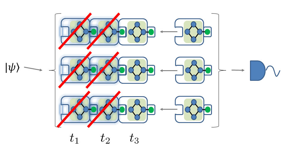
To allow communication between the processors, we entangle an ancillary light mode with the output node in the atomic cluster to form a qubrick which is a -composite cluster. The light mode of the qubrick can then be used to convey the output of the process performed on the atomic cluster contained in the brick to the next in the array (Fig.6). Given sufficient resources, the state can be processed in parallel using strings of qubricks. The total output from each of the strings can then be combined to give the final output.

In more detail, a typical process would proceed as follows. A state , is loaded onto the first cluster . Adaptive measurements are then applied to the atomic ensembles to process the state with outcome . A light mode , is added to to form the qubrick and the state is transferred to by a further measurement (Fig.7). Since the cluster and its associated entanglement has been destroyed in the measurement process the light pulse is free to carry the information to the next qubrick, without inadvertently entangling the atomic clusters belonging to different bricks. Another measurement transfers the state onto the first node of the atomic cluster, and a gate operation is performed by a new sequence of measurements yielding . A light mode , is added to to form a new qubrick and it carries the processed state is to the next cluster. Since each cluster applies some unitary transformation to the state, this process can be repeated until the desired output if achieved and the state is given by .
It is important to note that we do not claim that this procedure outperforms the error rate of large cluster arrays in general. What the qubrick scheme does guarantee, is that the loss of entanglement and therefore the errors accumulated in each quantum gate are constant. Then the errors that propagate through the computation are just proportional to the number of qubricks used. This is in contrast to the large cluster state in which the entanglement decays exponentially with the size of the cluster and hence errors accumulate rather quickly as the cluster size increases. Note however, that the error rate of particular geometries of large scale cluster states actually outperform the qubrick scheme i.e., for a 16-node square cluster. In this case the entanglement scales as , where is some constant. If we assume the error rate increases proportional to the degradation of entanglement then the errors scale as where is some constant that depends on the particular system in question. In the qubrick setting, to replicate this state exactly, we require four qubricks and the cumulative error then scales as , which is significantly worse. Here we do not propose that the qubricks mimic the large scale states exactly (since they can never beat the fundamental limit anyway). In this scheme, each qubrick and hence each quantum gate is initialized individually and only when it is required (Fig.(6)). These gates are then directly coupled to the light pulse carrying the output from previous processes. Our scheme removes the need for nodes serving as quantum wires to convey information around the cluster and eliminates any redundant nodes. In doing so we supress the exponential losses due to entanglement decay and hence reduce the error rate.
Furthermore, this method can be simplified to just one qubrick, if we loop the output from the brick back to the input in a similar manner to that proposed in [11]. In this scheme, the output from the first computation again gives . The atomic cluster is re-generated and the light mode is fed back into the input node where a different series of adaptive measurements is performed. This gives which is processed again until the desired unitary is enacted. This scheme eliminates the parallel element but it vastly decreases the number of resources required while maintaining a constant error rate. This time the error depends on the number of time the state is reused. This type of scheme could from the basis of a proof of principle demonstration of CV cluster state computation with atomic ensembles since it is achievable with currently available technology.
VII Conclusion
We have presented a scheme to produce a two-mode cluster state composed of an atomic ensemble and light pulse, called a composite cluster, via QND interactions and beamsplitters. We find that since both the atomic ensembles and light are initially Gaussian states and only Gaussian operations are performed, the procedure is well described by the covariance matrix formalism. From the covariance matrix we have confirmed that the states are indeed entangled using the PPT separability criterion. We have generalized our protocol, and given an explicit construction for multipartite composite cluster states composed of an arbitrary number of atomic and light modes. Using our composite clusters, we have proposed a new architecture for the one- way computer that reduces losses due to decay of localizable entanglement by preparing many separate clusters and using the light modes as information carriers between them. This scheme is experimentally feasible with current technology and has the potential for scalability since many of the resources can be re-used as many times as required.
Acknowledgements.
This research has been supported by the EU STREP project COMPAS FP7- ICT-2007-C-212008 under the FET-Open Programme, by the Scottish Universities Physics Alliance (SUPA) and by the Engineering and Physical Sciences Research Council (EPSRC).References
- [1] R. Raussendorf and H. J. Briegel, Phys. Rev. Lett 86, 5188 (2001).
- [2] M. A. Nielsen and I. L. Chuang, Quantum Computation and Quantum Information (Cambridge, 2000).
- [3] H. J. Briegel and R. Raussendorf, Phys. Rev. Lett. 86, 910 (2001).
- [4] D. L. Zhou, B. Zeng, Z. Xu, and C. P. Sun, Phys. Rev. A 68, 062303 (2003)
- [5] N. C. Meniucci et al, Phys. Rev. Lett 97, 110501 (2006).
- [6] P. van Loock, C. Weedbrook, and M. Gu, Phys. Rev. A 76, 060301 (2007).
- [7] J. Zhang and S. L. Braustein, Phys. Rev. A 73, 032318 (2006).
- [8] M. Gu et al, Phys. Rev. A, 79, 062318 (2009).
- [9] N. C. Menicucci, S. T. Flammia, and O. Pfister, Phys. Rev. Lett. 101, 130501 (2008).
- [10] S. T. Flammia, N. C. Menicucci, and O. Pfister, J. Phys. B 42, 114009 (2009).
- [11] N. C. Menicucci, X. Ma, and T. C. Ralph, Phys. Rev. Lett. 104, 250503 (2010).
- [12] N. C. Menicucci, Phys. Rev. A 83, 062314 (2011)
- [13] M. A. Nielsen, Phys. Rev. Lett 93, 040503 (2004).
- [14] D. E. Browne, and T. Rudolph, Phys. Rev. Lett 95, 010501, (2005).
- [15] L.-M. Duan and R. Raussendorf, Phys. Rev. Lett 95, 080503 (2005).
- [16] S. L. Braunstein, Phys. Rev. A 71, 055801 (2005).
- [17] B. Yurke, J. Opt. Soc. Am. B 2, 732 (1985).
- [18] Radim Filip, Petr Marek, and Ulrik L. Andersen, Phys. Rev. A 71, 042308 (2005).
- [19] J. Yoshikawa et al, Phys. Rev. Lett 101, 250501 (2008).
- [20] D. F. Milne, and N. V. Korolkova, Generation of atomic cluster states by QND measurements,
- [21]
D. F. Milne, and N. V. Korolkova, Generation
of hybrid cluster states using non-demolition measurements,
- [22] J. Stasinska, C. Rodó, S. Paganelli, G. Birk, and A. Sanpera, Phys. Rev. A 80, 062304 (2009).
- [23] J. Stasinska, S. Paganelli, C. Rodó, and A. Sanpera, arXiv:10070403v3 [quant-ph] (2011).
- [24] M. Ohliger, K. Kieling, and J. Eisert, Phys. Rev. A 82, 042336 (2010).
- [25] B. Julsgaard, A. Kozhekin and E. Polzik, Nature 413 (2001).
- [26] B. Julsgaard, Entanglement and Quantum Interactions with Macroscopic Gas Samples. PhD thesis, University of Aarhus, Denmark (2003).
- [27] E. Knill, R. Laflamme and G. J. Milburn, Nature (London) 409, 46 (2001)
- [28] G. Giedke, and J. I. Cirac. Phys. Rev. A 66, 032316 (2002).
- [29] S. L. Braunstein, and P. van Loock, Rev. Mod. Phys, 77, 513 (2005).
- [30] G. Adesso, and F. Illuminati, arXiv: [quant-ph] 0510052v2 (2007).
- [31] G. Adesso, and F. Illuminati, J. Phys. A: Math Theor, 40 7821 (2007).
- [32] A. Peres, Phys. Rev. Lett 77, 1413 (1996).
- [33] R. Horodecki, P. Horodecki, and M. Horodecki, Phys. Rev. Lett 210, 377 (1996).
- [34] J. Williamson, Am. J. Math 58, 141 (1936).
- [35] R. Simon, Phys. Rev. Lett 84, 2726 (2000).
- [36] R. F. Werner and M. M, Wolf, Phys. Rev. Lett 86, 3658 (2001).
- [37] G. Vidal, and R. F. Werner, Phys. Rev. A 65, 032314 (2002).
- [38] M. B. Plenio, Phys. Rev. Lett 95, 090503 (2005).
- [39] L-.H. Duan, G. Giedke, J. I. Cirac, and P. Zoller, Phys. Rev. Lett 84, 2722 (2000).
- [40] P. van Loock, and A. Furusawa, Phys. Rev. A 67, 052315 (2003).
- [41] C. Horsman, K.L. Brown, W. J. Munro, and V.M. Kendon, Phys. Rev. A 83, 042327 (2011)
Appendix A Explicit covariance matrices for two-mode composite cluster state
Here we give the explicit CM for the two-mode composite cluster state. Computing yields the CM:
| (28) |
However, this has not produced the required entanglement between the atomic and light mode. Homodyning the interaction pulses produces the required correlations. In terms of covariance matrices, this amounts to the operation
| (29) |
which traces out the interaction light modes and to leave us with a matrix representing only the atomic and light modes that are part of the cluster:
| (30) |
This final CM represents the state (up to a known displacement that depends on the measurement outcome) of the two-mode composite cluster. Here, the upper left block represents the atomic mode, the lower right is the light mode and the off diagonal blocks are the correlations between them.