跳到论文正文
W Papers独立论文阅读器 arXiv:1202.1119 论文正文 计算阅读时间 · 0%
引用这篇论文根据当前论文元数据生成,正式投稿前建议核对。


License: arXiv.org perpetual non-exclusive license
arXiv:1202.1119v2 [cs.LG] 18 Oct 2012

Cramér-Rao–Type Bounds for Sparse Bayesian LearningThanks: The authors are with the Dept. of Electrical Communication Eng. at IISc, Bangalore, India. (e-mails: {ranjitha.p, cmurthy}@ece.iisc.ernet.in)Thanks: Copyright (c) 2012 IEEE. Personal use of this material is permitted. However, permission to use this material for any other purposes must be obtained from the IEEE by sending a request to pubs-permissions@ieee.org.

Ranjitha Prasad and Chandra R. Murthy Senior Member, IEEE Affiliation:
Abstract

In this paper, we derive Hybrid, Bayesian and Marginalized Cramér-Rao lower bounds (HCRB, BCRB and MCRB) for the single and multiple measurement vector Sparse Bayesian Learning (SBL) problem of estimating compressible vectors and their prior distribution parameters. We assume the unknown vector to be drawn from a compressible Student-tt prior distribution. We derive CRBs that encompass the deterministic or random nature of the unknown parameters of the prior distribution and the regression noise variance. We extend the MCRB to the case where the compressible vector is distributed according to a general compressible prior distribution, of which the generalized Pareto distribution is a special case. We use the derived bounds to uncover the relationship between the compressibility and Mean Square Error (MSE) in the estimates. Further, we illustrate the tightness and utility of the bounds through simulations, by comparing them with the MSE performance of two popular SBL-based estimators. It is found that the MCRB is generally the tightest among the bounds derived and that the MSE performance of the Expectation-Maximization (EM) algorithm coincides with the MCRB for the compressible vector. Through simulations, we demonstrate the dependence of the MSE performance of SBL based estimators on the compressibility of the vector for several values of the number of observations and at different signal powers.

Index Terms:
Sparse Bayesian learning, mean square error, Cramér-Rao lower bounds, expectation maximization.

I Introduction

Recent results in the theory of compressed sensing have generated immense interest in sparse vector estimation problems, resulting in a multitude of successful practical signal recovery algorithms. In several applications, such as the processing of natural images, audio, and speech, signals are not exactly sparse, but compressible, i.e., the magnitudes of the sorted coefficients of the vector follow a power law decay [1]. In [2] and [3], the authors show that random vectors drawn from a special class of probability distribution functions (pdf) known as compressible priors result in compressible vectors. Assuming that the vector to be estimated (henceforth referred to as the unknown vector) has a compressible prior distribution enables one to formulate the compressible vector recovery problem in the Bayesian framework, thus allowing the use of Sparse Bayesian Learning (SBL) techniques [4]. In his seminal work, Tipping proposed an SBL algorithm for estimating the unknown vector, based on the Expectation Maximization (EM) and McKay updates [4]. Since these update rules are known to be slow, fast update techniques are proposed in [5]. A duality based algorithm for solving the SBL cost function is proposed in [6], and ℓ1−ℓ2\ell_{1}-\ell_{2} based reweighting schemes are explored in [7]. Such algorithms have been successfully employed for image/visual tracking [8], neuro-imaging [9, 10], beamforming [11], and joint channel estimation and data detection for OFDM systems [12].
Many of the aforementioned papers study the complexity, convergence and support recovery properties of SBL based estimators (e.g., [5, 6]). In [3], the general conditions required for the so-called instance optimality of such estimators are derived. However, it is not known whether these recovery algorithms are optimal in terms of the Mean Square Error (MSE) in the estimate or by how much their performance can be improved. In the context of estimating sparse signals, Cramér-Rao lower bounds on the MSE performance are derived in [13, 14, 15]. However, to the best of our knowledge, none of the existing works provide a lower bound on the MSE performance of compressible vector estimation. Such bounds are necessary, as they provide absolute yardsticks for comparative analysis of estimators, and may also be used as a criterion for minimization of MSE in certain problems [16]. In this paper, we close this gap in theory by providing Cramér-Rao type lower bounds on the MSE performance of estimators in the SBL framework.

As our starting point, we consider a linear Single Measurement Vector (SMV) SBL model given by

𝐲=𝚽​𝐱+𝐧,\mathbf{y}=\bm{\Phi}\mathbf{x}+\mathbf{n}, (1)

where the observations 𝐲∈ℝN\mathbf{y}\in\mathbb{R}^{N} and the measurement matrix 𝚽∈ℝN×L\bm{\Phi}\in\mathbb{R}^{N\times L} are known, and 𝐱∈ℝL\mathbf{x}\in\mathbb{R}^{L} is the unknown sparse/compressible vector to be estimated [17]. Each component of the additive noise 𝐧∈ℝN\mathbf{n}\in\mathbb{R}^{N} is white Gaussian, distributed as 𝒩⁡(0,σ2)\mathcal{N}(0,\sigma^{2}), where the variance σ2\sigma^{2} may be known or unknown. The SMV-SBL system model in (1) can be generalized to a linear Multiple Measurement Vector (MMV) SBL model given by

𝐓=𝚽​𝐖+𝐕.\mathbf{T}=\bm{\Phi}\mathbf{W}+\mathbf{V}. (2)

Here, 𝐓∈ℝN×M\mathbf{T}\in\mathbb{R}^{N\times M} represents the MM observation vectors, the columns of 𝐖∈ℝL×M\mathbf{W}\in\mathbb{R}^{L\times M} are the MM sparse/compressible vectors with a common underlying distribution, and each column of 𝐕∈ℝN×M\mathbf{V}\in\mathbb{R}^{N\times M} is modeled similar to 𝐧\mathbf{n} in (1) [18].
In typical compressible vector estimation problems, 𝚽\bm{\Phi} is underdetermined (N<LN<L), rendering the problem ill-posed. Bayesian techniques circumvent this problem by using a prior distribution on the compressible vector as a regularization, and computing the corresponding posterior estimate. To incorporate a compressible prior in (1) and (2), SBL uses a two-stage hierarchical model on the unknown vector, as shown in Fig. 1. Here, 𝐱∼𝒩⁡(0,𝚼)\mathbf{x}\sim\mathcal{N}(0,\bm{\Upsilon}), where the diagonal matrix 𝚼\bm{\Upsilon} contains the hyperparameters 𝜸=[γ1,…,γL]T\bm{\gamma}=[\gamma_{1},\ldots,\gamma_{L}]^{T} as its diagonal elements. Further, an Inverse Gamma (IG) hyperprior is assumed for 𝜸\bm{\gamma} itself, because it leads to a Student-tt prior on the vector 𝐱\mathbf{x}, which is known to be compressible [4].11 1 The IG hyperprior is conjugate to the Gaussian pdf [4]. In scenarios where the noise variance is unknown and random, an IG prior is used for the distribution of the noise variance as well. For the system model in (2), every compressible vector 𝐰i∼𝒩⁡(0,𝚼)\mathbf{w}_{i}\sim\mathcal{N}(0,\bm{\Upsilon}), i.e., the MM compressible vectors are governed by a common 𝚼\bm{\Upsilon}.

x j y i σ 2 j = 1 : L i = 1 : N k = 1 : N ⁢ I G ( c , d ) n k N ( 0 , σ 2 ) γ j | y ∼ x N ( ⁢ Φ x , ⁢ σ 2 I × N N ) N ( 0 , γ j ) ⁢ I G ( ν , ⁢ / ν 2 λ )
Figure 1: Graphical model for SBL: Two stage hierarchical model with the compressible vector taking a conditional Gaussian distribution and the hyperparameters taking an Inverse Gamma distribution. The noise is modeled as white Gaussian distributed, with the noise variance modeled as deterministic/random and known or unknown.

It is well known that the Cramér-Rao Lower Bound (CRLB) provides a fundamental limit on the MSE performance of unbiased estimators [19] for deterministic parameter estimation. For the estimation problem in SBL, an analogous bound known as the Bayesian Cramér-Rao Bound (BCRB) is used to obtain lower bounds [20], by incorporating the prior distribution on the unknown vector. If the unknown vector consists of both deterministic and random components, Hybrid Cramér-Rao Bounds (HCRB) are derived [21].

In SBL, the unknown vector estimation problem can also be viewed as a problem involving nuisance parameters. Since the assumed hyperpriors are conjugate to the Gaussian likelihood, the marginalized distributions have a closed form and the Marginalized Cramér-Rao Bounds (MCRB) [22] can be derived. For example, in the SBL hyperparameter estimation problem, 𝐱\mathbf{x} itself can be considered a nuisance variable and marginalized from the joint distribution, p𝐘,𝐗|𝜸​(𝐲,𝐱|𝜸){p}_{\mathbf{Y},\mathbf{X}|\bm{\gamma}}(\mathbf{y},\mathbf{x}|\bm{\gamma}), to obtain the log likelihood as

log∫𝐱p𝐘,𝐗|Γ(𝐲,𝐱|𝜸)d𝐱=−(log⁡|𝚺y|+𝐲T​𝚺y−1​𝐲)2,\log\int_{\mathbf{x}}{p}_{\mathbf{Y},\mathbf{X}|\Gamma}(\mathbf{y},\mathbf{x}|\bm{\gamma})\mathrm{d}\mathbf{x}=\frac{-(\log|\bm{\Sigma}_{y}|+\mathbf{y}^{T}\bm{\Sigma}_{y}^{-1}\mathbf{y})}{2}, (3)

where 𝚺y=σ2​𝐈N×N+𝚽​𝚼​𝚽T\bm{\Sigma}_{y}=\sigma^{2}\mathbf{I}_{N\times N}+\bm{\Phi}\bm{\Upsilon}\bm{\Phi}^{T} [23].

: deterministic γ MCRB from p ( y , x ) : random x : marginalized γ MCRB from p ( y , γ ) : deterministic γ : random x = , θ [ γ T x T ] T : marginalized x : random γ : random x BCRB from p ( y , x , γ ) HCRB from p ( y , x , γ )
Figure 2: Summary of the lower bounds derived in this work when noise variance is assumed to be known.

The goal of this paper is to derive Cramér-Rao type lower bounds on the MSE performance of estimators based on the SBL framework. Our contributions are as follows:

  • •

    Under the assumption of known noise variance, we derive the HCRB and the BCRB for the unknown vector 𝜽=[𝐱T,𝜸T]T\bm{\theta}=[\mathbf{x}^{T},\bm{\gamma}^{T}]^{T}, as indicated in the left half of Fig. 2.

  • •

    When the noise variance is known, we marginalize nuisance variables (𝜸\bm{\gamma} or 𝐱\mathbf{x}) and derive the corresponding MCRB, as indicated in the right half of Fig. 2. Since the MCRB is a function of the parameters of the hyperprior (and hence is an offline bound), it yields insights into the relationship between the MSE performance of the estimators and the compressibility of 𝐱\mathbf{x}.

  • •

    In the unknown noise variance case, we derive the BCRB, HCRB and MCRB for the unknown vector 𝜽=[𝐱T,𝜸T,σ2]T\bm{\theta}=[\mathbf{x}^{T},\bm{\gamma}^{T},\sigma^{2}]^{T}, as indicated in Fig. 3.

  • •

    We derive the MCRB for a general parametric form of the compressible prior [3] and deduce lower bounds for two of the well-known compressible priors, namely, the Student-tt and generalized double Pareto distributions.

  • •

    Similar to the SMV-SBL case, we derive the BCRB, HCRB and MCRB for the MMV-SBL model in (2).

Through numerical simulations, we show that the MCRB on the compressible vector 𝐱\mathbf{x} is the tightest lower bound, and that the MSE performance of the EM algorithm achieves this bound at high SNR and as N→LN\rightarrow L. The techniques used to derive the bounds can be extended to handle different compressible prior pdfs used in literature [2]. These results provide a convenient and easy-to-compute benchmark for comparing the performance of the existing estimators, and in some cases, for establishing their optimality in terms of the MSE performance.

: deterministic γ : random x : random σ 2 : random γ : random x : random σ 2 : deterministic γ : marginalized x : deterministic σ 2 = θ [ γ T , x T , σ 2 ] T p ( y , γ , σ 2 ) p ( y , x , σ 2 , γ ) p ( y , x , σ 2 , γ )
Figure 3: Different modeling assumptions and the corresponding bounds derived in this work when noise variance is assumed to be unknown.

The rest of this paper is organized as follows. In Sec. II, we provide the basic definitions and describe the problem set up. In Secs. III and IV, we derive the lower bounds for the cases shown in Figs. 2 and 3, respectively. The bounds are extended to the MMV-SBL signal model in Sec. V. The efficacy of the lower bounds is graphically illustrated through simulation results in Sec. VI. We provide some concluding remarks in Sec. VII. In the Appendix, we provide proofs for the Propositions and Theorems stated in the paper.

Notation: In the sequel, boldface small letters denote vectors and boldface capital letters denote matrices. The symbols (⋅)T(\cdot)^{T} and |⋅||\cdot| denote the transpose and determinant of a matrix, respectively. The empty set is represented by ∅\emptyset, and Γ⁡(⋅)\Gamma(\cdot) denotes the Gamma function. The function pX​(x){p}_{X}(x) represents the pdf of the random variable XX evaluated at its realization xx. Also, diag​(𝐚)\mbox{diag}(\mathbf{a}) stands for a diagonal matrix with entries on the diagonal given by the vector 𝐚\mathbf{a}. The symbol ∇𝜽\nabla_{\bm{\theta}} is the gradient with respect to (w.r.t.) the vector 𝜽\bm{\theta}. The expectation w.r.t. a random variable XX is denoted as 𝔼X​(⋅)\mathbb{E}_{X}(\cdot). Also, 𝐀⪰𝐁\mathbf{A}\succeq\mathbf{B} denotes that 𝐀−𝐁\mathbf{A}-\mathbf{B} is positive semidefinite, and 𝐀⊗𝐁\mathbf{A}\otimes\mathbf{B} is the Kronecker product of the two matrices 𝐀\mathbf{A} and 𝐁\mathbf{B}.

II Preliminaries

As a precursor to the sections that follow, we define the MSE matrix and the Fisher Information Matrix (FIM) [19], and state the assumptions under which we derive the lower bounds in this paper. Consider a general estimation problem where the unknown vector 𝜽∈ℝn\bm{\theta}\in\mathbb{R}^{n} can be split into sub-vectors 𝜽=[𝜽rT,𝜽dT]T\bm{\theta}=[\bm{\theta}_{r}^{T},\penalty\ \bm{\theta}_{d}^{T}]^{T}, where 𝜽r∈ℝm\bm{\theta}_{r}\in\mathbb{R}^{m} consists of random parameters distributed according to a known pdf, and 𝜽d∈ℝn−m\bm{\theta}_{d}\in\mathbb{R}^{n-m} consists of deterministic parameters. Let 𝜽^​(𝐲)\hat{\bm{\theta}}(\mathbf{y}) denote the estimator of 𝜽\bm{\theta} as a function of the observations 𝐲\mathbf{y}. The MSE matrix 𝐄𝜽\mathbf{E}^{\bm{\theta}} is defined as

𝐄𝜽≜𝔼𝐘,Θr​[(𝜽−𝜽^​(𝐲))​(𝜽−𝜽^​(𝐲))T],\mathbf{E}^{\bm{\theta}}\triangleq\mathbb{E}_{\mathbf{Y},\Theta_{r}}\left[(\bm{\theta}-\hat{\bm{\theta}}(\mathbf{y}))(\bm{\theta}-\hat{\bm{\theta}}(\mathbf{y}))^{T}\right], (4)

where Θr\Theta_{r} denotes the random parameters to be estimated, whose realization is given by 𝜽r\bm{\theta}_{r}. The first step in obtaining Cramér-Rao type lower bounds is to derive the FIM 𝐈𝜽\mathbf{I}^{\bm{\theta}} [19]. Typically, 𝐈𝜽\mathbf{I}^{\bm{\theta}} is expressed in terms of the individual blocks of submatrices, where the (i​j)th(ij)^{\text{th}} block is given by

𝐈i​j𝜽≜−𝔼𝐘,Θr​[∇𝜽i∇𝜽jT​log⁡p𝐘,Θr;Θd​(𝐲,𝜽r,𝜽d)].\mathbf{I}^{\bm{\theta}}_{ij}\triangleq-\mathbb{E}_{\mathbf{Y},\Theta_{r}}[\nabla_{\bm{\theta}_{i}}\nabla_{\bm{\theta}_{j}}^{T}\log{p}_{\mathbf{Y},\Theta_{r};\Theta_{d}}(\mathbf{y},\bm{\theta}_{r};\bm{\theta}_{d})]. (5)

In this paper, we use the notation 𝐈𝜽\mathbf{I}^{\bm{\theta}} to represent the FIM under the different modeling assumptions. For example, when 𝜽r≠∅\bm{\theta}_{r}\neq\emptyset and 𝜽d≠∅\bm{\theta}_{d}\neq\emptyset, 𝐈𝜽\mathbf{I}^{\bm{\theta}} represents a Hybrid Information Matrix (HIM). When 𝜽r≠∅\bm{\theta}_{r}\neq\emptyset and 𝜽d=∅\bm{\theta}_{d}=\emptyset, 𝐈𝜽\mathbf{I}^{\bm{\theta}} represents a Bayesian Information matrix (BIM). Assuming that the MSE matrix 𝐄𝜽\mathbf{E}^{\bm{\theta}} exists and the FIM is non-singular, a lower bound on the MSE matrix 𝐄𝜽\mathbf{E}^{\bm{\theta}} is given by the inverse of the FIM:

𝐄𝜽⪰(𝐈𝜽)−1.\mathbf{E}^{\bm{\theta}}\succeq\left(\mathbf{I}^{\bm{\theta}}\right)^{-1}. (6)

It is easy to verify that the underlying pdfs considered in the SBL model satisfy the regularity conditions required for computing the FIM (see Sec. 5.2.3 in [22]).
We conclude this section by making one useful observation about the FIM in the SBL problem. An assumption in the SMV-SBL framework is that 𝐱\mathbf{x} and 𝐧\mathbf{n} are independent of each other (for the MMV-SBL model, 𝐓\mathbf{T} and 𝐖\mathbf{W} are independent). This assumption is reflected in the graphical model in Fig. 1, where the compressible vector 𝐱\mathbf{x} (and its attribute 𝜸\bm{\gamma}) and the noise component 𝐧\mathbf{n} (and its attribute σ2\sigma^{2}) are on unconnected branches. Due to this, a submatrix of the FIM is of the form

𝐈𝜸​ξ𝜽=−𝔼𝐗,𝐘,Γ,Ξ[∇𝜸∇ξ{logp𝐘|𝐗,Ξ(𝐲|𝐱,ξ)\displaystyle\mathbf{I}^{\bm{\theta}}_{\bm{\gamma}\xi}=-\mathbb{E}_{\mathbf{X},\mathbf{Y},\Gamma,\Xi}\left[\nabla_{\bm{\gamma}}\nabla_{\xi}\left\{\log{p}_{\mathbf{Y}|\mathbf{X},\Xi}(\mathbf{y}|\mathbf{x},\xi)\right.\right.
+logp𝐗,Γ(𝐱,𝜸)+logpΞ(ξ)}],\displaystyle\left.\left.+\log{p}_{\mathbf{X},\Gamma}(\mathbf{x},\bm{\gamma})+\log{p}_{\Xi}(\xi)\right\}\right], (7)

where there are no terms in which both 𝜸\bm{\gamma} and ξ=σ2\xi=\sigma^{2} are jointly present. Hence, the corresponding terms in the above mentioned submatrix are always zero. This is formally stated in the following Lemma.

Lemma 1

When 𝛉i=𝛄\bm{\theta}_{i}=\bm{\gamma} and 𝛉j=σ2\bm{\theta}_{j}=\sigma^{2}, the (i​j)th(ij)^{\text{th}} block matrix of the FIM 𝐈𝛉\mathbf{I}^{\bm{\theta}} given by (5) simplifies to 𝐈i​j𝛉=𝟎L×1\mathbf{I}^{\bm{\theta}}_{ij}=\mathbf{0}_{L\times 1}, i.e., to an all zero vector.

III SMV-SBL: Lower Bounds when σ2\sigma^{2} is Known

In this section, we derive lower bounds for the system model in (1) for the scenarios in Fig. 2, where the unknown vector is 𝜽=[𝐱T,𝜸T]T\bm{\theta}=[\mathbf{x}^{T},\bm{\gamma}^{T}]^{T}. We examine different modeling assumptions on 𝜸\bm{\gamma} and derive the corresponding lower bounds.

III-A Bounds from the Joint pdf

III-A1 HCRB for 𝜽=[𝐱T,𝜸T]T\bm{\theta}=[\mathbf{x}^{T},\bm{\gamma}^{T}]^{T}

In this subsection, we consider the unknown variables as a hybrid of a deterministic vector 𝜸\bm{\gamma} and a random vector 𝐱\mathbf{x} distributed according to a Gaussian distribution parameterized by 𝜸\bm{\gamma}. Using the assumptions and notation in the previous section, we obtain the following proposition.

Proposition 1

For the signal model in (1), the HCRB on the MSE matrix 𝐄𝛉\mathbf{E}^{\bm{\theta}} of the unknown vector 𝛉=[𝐱T,𝛄T]T\bm{\theta}=[\mathbf{x}^{T},\bm{\gamma}^{T}]^{T} with the parameterized distribution of the compressible signal 𝐱\mathbf{x} given by 𝒩⁡(0,𝚼)\mathcal{N}(0,\bm{\Upsilon}), and with 𝛄\bm{\gamma} modeled as unknown and deterministic, is given by 𝐄𝛉⪰(𝐇𝛉)−1\mathbf{E}^{\bm{\theta}}\succeq(\mathbf{H}^{\bm{\theta}})^{-1}, where

𝐇𝜽≜[𝐇𝜽​(𝐱)𝐇𝜽​(𝐱,𝜸)(𝐇𝜽​(𝐱,𝜸))T𝐇𝜽​(𝜸)]=\displaystyle\mathbf{H}^{\bm{\theta}}\triangleq\begin{bmatrix}\mathbf{H}^{\bm{\theta}}(\mathbf{x})&\mathbf{H}^{\bm{\theta}}(\mathbf{x},\bm{\gamma})\\ (\mathbf{H}^{\bm{\theta}}(\mathbf{x},\bm{\gamma}))^{T}&\mathbf{H}^{\bm{\theta}}(\bm{\gamma})\end{bmatrix}=
[(𝚽T​𝚽σ2+𝚼−1)𝟎L×L𝟎L×Ldiag​(2​γ12, 2​γ22,…, 2​γL2)−1].\displaystyle\begin{bmatrix}\left(\frac{\bm{\Phi}^{T}\bm{\Phi}}{\sigma^{2}}+\bm{\Upsilon}^{-1}\right)&\mathbf{0}_{L\times L}\\ \mathbf{0}_{L\times L}&\textnormal{diag}({2\gamma_{1}^{2}},\penalty\ {2\gamma_{2}^{2}},\penalty\ \ldots,\penalty\ {2\gamma_{L}^{2}})^{-1}\end{bmatrix}. (8)

Proof: See Appendix -A.

Note that the lower bound on the estimate of 𝐱\mathbf{x} depends on the prior information through the diagonal matrix 𝚼\bm{\Upsilon}. In the SBL problem, the realization of the random parameter 𝜸\bm{\gamma} has to be used to compute the bound above, and hence, it is referred to as an online bound. Also, the lower bound on the MSE matrix of 𝐱\mathbf{x} is 𝐄𝜽⪰(𝚽T​𝚽σ2+𝚼−1)−1\mathbf{E}^{\bm{\theta}}\succeq\left(\frac{\bm{\Phi}^{T}\bm{\Phi}}{\sigma^{2}}+\bm{\Upsilon}^{-1}\right)^{-1}, which is the same as the lower bound on the error covariance of the Baye’s vector estimator for a linear model (see Theorems 10.2 and 10.3 in [19]), and is achievable by the MMSE estimator when 𝚼=diag​(γ1,…,γL)\bm{\Upsilon}=\mbox{diag}(\gamma_{1},\ldots,\gamma_{L}) is known.

III-A2 BCRB for 𝜽=[𝐱T,𝜸T]T\bm{\theta}=[\mathbf{x}^{T},\bm{\gamma}^{T}]^{T}

For deriving the BCRB, a hyperprior distribution is considered on 𝜸\bm{\gamma}, and the resulting 𝐱\mathbf{x} is viewed as being drawn from a compressible prior distribution. The most commonly used hyperprior distribution in the literature is the IG distribution [4], where γi,i=1,2,…,L\gamma_{i},i=1,2,\ldots,L are distributed as ℐ​𝒢​(ν2,ν2​λ)\mathcal{IG}\left(\frac{\nu}{2},\frac{\nu}{2\lambda}\right), given by

pΓ​(γi)≜(Γ⁡(ν2))−1​(ν2​λ)ν2​γi(−ν2−1)​exp⁡{−ν2​λ​γi},{p}_{\Gamma}(\gamma_{i})\triangleq\left(\Gamma\left(\frac{\nu}{2}\right)\right)^{-1}\left(\frac{\nu}{2\lambda}\right)^{\frac{\nu}{2}}{\gamma_{i}^{\left(-\frac{\nu}{2}-1\right)}\exp\left\{-\frac{\nu}{2\lambda\gamma_{i}}\right\}}, (9)

where γi∈(0,∞),ν,λ>0\gamma_{i}\in(0,\infty),\penalty\ \penalty\ \nu,\lambda>0. Using the definitions and notation in the previous section, we state the following proposition.

Proposition 2

For the signal model in (1), the BCRB on the MSE matrix 𝐄𝛉\mathbf{E}^{\bm{\theta}} of the unknown random vector 𝛉=[𝐱T,𝛄T]T\bm{\theta}=[\mathbf{x}^{T},\bm{\gamma}^{T}]^{T}, where the conditional distribution of the compressible signal 𝐱|𝛄\mathbf{x}|\bm{\gamma} is 𝒩⁡(0,𝚼)\mathcal{N}(0,\bm{\Upsilon}), and the hyperprior distribution on 𝛄\bm{\gamma} is ∏i=1Lℐ​𝒢​(ν2,ν2​λ)\prod_{i=1}^{L}\mathcal{IG}\left(\frac{\nu}{2},\frac{\nu}{2\lambda}\right), is given by 𝐄𝛉⪰(𝐁𝛉)−1\mathbf{E}^{\bm{\theta}}\succeq(\mathbf{B}^{\bm{\theta}})^{-1}, where

𝐁𝜽≜[𝐁𝜽​(𝐱)𝐁𝜽​(𝐱,𝜸)(𝐁𝜽​(𝐱,𝜸))T𝐁𝜽​(𝜸)]=\displaystyle\mathbf{B}^{\bm{\theta}}\triangleq\begin{bmatrix}\mathbf{B}^{\bm{\theta}}(\mathbf{x})&\mathbf{B}^{\bm{\theta}}(\mathbf{x},\bm{\gamma})\\ (\mathbf{B}^{\bm{\theta}}(\mathbf{x},\bm{\gamma}))^{T}&\mathbf{B}^{\bm{\theta}}(\bm{\gamma})\end{bmatrix}=
[(𝚽T​𝚽σ2+λ​𝐈L×L)𝟎L×L𝟎L×Lλ2​(ν+2)​(ν+7)2​ν​𝐈L×L].\displaystyle\begin{bmatrix}\left(\frac{\bm{\Phi}^{T}\bm{\Phi}}{\sigma^{2}}+{\lambda}\mathbf{I}_{L\times L}\right)&\mathbf{0}_{L\times L}\\ \mathbf{0}_{L\times L}&\frac{\lambda^{2}(\nu+2)(\nu+7)}{2\nu}\mathbf{I}_{L\times L}\end{bmatrix}. (10)

Proof: See Appendix -B.

It can be seen from 𝐁𝜽\mathbf{B}^{\bm{\theta}} that the lower bound on the MSE of 𝜸^​(𝐲)\hat{\bm{\gamma}}(\mathbf{y}) is a function of the parameters of the IG prior on 𝜸\bm{\gamma}, i.e., a function of ν\nu and λ\lambda, and it can be computed without the knowledge of realization of 𝜸\bm{\gamma}. Thus, it is an offline bound.

III-B Bounds from Marginalized Distributions

III-B1 MCRB for 𝜽=[𝜸]\bm{\theta}=[\bm{\gamma}]

Here, we derive the MCRB for 𝜽=[𝜸]\bm{\theta}=[\bm{\gamma}], where 𝜸\bm{\gamma} is an unknown deterministic parameter. This requires the marginalized distribution p𝐘;𝜸​(𝐲,𝜸){p}_{\mathbf{Y};\bm{\gamma}}(\mathbf{y};\bm{\gamma}), which is obtained by considering 𝐱\mathbf{x} as a nuisance variable and marginalizing it out of the joint distribution p𝐗,𝐘;𝜸​(𝐱,𝐲,𝜸){p}_{\mathbf{X},\mathbf{Y};\bm{\gamma}}(\mathbf{x},\mathbf{y};\bm{\gamma}), to obtain (3). Since 𝜸\bm{\gamma} is a deterministic parameter, the pdf p𝐘;𝜸​(𝐲,𝜸){p}_{\mathbf{Y};\bm{\gamma}}(\mathbf{y};\bm{\gamma}) must satisfy the regularity condition in [19]. We have the following theorem.

Theorem 1

For the signal model in (1), the log likelihood function log⁡p𝐘;𝛄​(𝐲,𝛄)\log{p}_{\mathbf{Y};\bm{\gamma}}(\mathbf{y};\bm{\gamma}) satisfies the regularity conditions in [19]. Further, the MCRB on the MSE matrix 𝐄𝛄\mathbf{E}^{\bm{\gamma}} of the unknown deterministic vector 𝛉=[𝛄]\bm{\theta}=[\bm{\gamma}] is given by 𝐄𝛄⪰(𝐌𝛄)−1\mathbf{E}^{\bm{\gamma}}\succeq({\mathbf{M}^{\bm{\gamma}}})^{-1}, where the (i​j)th(ij)^{\text{th}} element of 𝐌𝛄\mathbf{M}^{\bm{\gamma}} is given by

𝐌i​j𝜸=12​(ΦjT​𝚺y−1​Φi)2,\mathbf{M}^{\bm{\gamma}}_{ij}=\frac{1}{2}(\Phi_{j}^{T}\bm{\Sigma}_{y}^{-1}\Phi_{i})^{2}, (11)

for 1≤i,j≤L1\leq i,j\leq L, where Φi\Phi_{i} is the ithi^{\text{th}} column of 𝚽\bm{\Phi}, and 𝚺y=σ2​𝐈N×N+𝚽​𝚼​𝚽T\bm{\Sigma}_{y}=\sigma^{2}\mathbf{I}_{N\times N}+\bm{\Phi}\bm{\Upsilon}\bm{\Phi}^{T}, as defined earlier.

Proof: See Appendix -C.

To intuitively understand (11), we consider a special case of 𝚽T​𝚽=N​𝐈N×N\bm{\Phi}^{T}\bm{\Phi}=N\mathbf{I}_{N\times N}, and use the Woodbury formula to simplify 𝚺y−1\bm{\Sigma}_{y}^{-1}, to obtain the (i​i)th(ii)^{\text{th}} entry of the matrix 𝐌𝜸\mathbf{M}^{\bm{\gamma}} as

𝐌i​i𝜸=2​(σ2N+γi)−2.\displaystyle\mathbf{M}^{\bm{\gamma}}_{ii}=2\left(\frac{\sigma^{2}}{N}+\gamma_{i}\right)^{-2}. (12)

Hence, the error in γi\gamma_{i} is bounded as 𝐄i​i𝜸≥2​(σ2N+γi)2\mathbf{E}^{\bm{\gamma}}_{ii}\geq 2\left(\frac{\sigma^{2}}{N}+\gamma_{i}\right)^{2}. As N→∞N\rightarrow\infty, the bound reduces to 2​γi22\gamma_{i}^{2}, which is the same as the lower bound on the estimate of 𝜸\bm{\gamma} obtained as the lower-right submatrix in (8). For finite NN, the MCRB is tighter than the HCRB.

III-B2 MCRB for 𝜽=[𝐱]\bm{\theta}=[\mathbf{x}]

In this subsection, we assume a hyperprior on 𝜸\bm{\gamma}, which leads to a joint distribution of 𝐱\mathbf{x} and 𝜸\bm{\gamma}, from which 𝜸\bm{\gamma} can be marginalized. Further, assuming specific forms for the hyperprior distribution can lead to a compressible prior on 𝐱\mathbf{x}. For example, assuming an IG hyperprior on 𝜸\bm{\gamma} leads to an 𝐱\mathbf{x} with a Student-tt distribution. Sampling from a Student-tt distribution with parameters ν\nu and λ\lambda results in a ν\nu-compressible 𝐱\mathbf{x} [2]. The Student-tt prior is given by

p𝐗​(𝐱)≜(Γ⁡((ν+1)/2)Γ⁡(ν/2))L​(λπ​ν)L2​∏i=1L(1+λ​xi2ν)−ν+12,{p}_{\mathbf{X}}(\mathbf{x})\triangleq\left(\frac{\Gamma((\nu+1)/2)}{\Gamma(\nu/2)}\right)^{L}\left(\frac{\lambda}{\pi\nu}\right)^{\frac{L}{2}}\prod_{i=1}^{L}\left(1+\frac{\lambda x_{i}^{2}}{\nu}\right)^{-\frac{\nu+1}{2}}, (13)

where xi∈(−∞,∞),ν,λ>0x_{i}\in(-\infty,\infty),\penalty\ \penalty\ \nu,\lambda>0, ν\nu represents the number of degrees of freedom and λ\lambda represents the inverse variance of the distribution. Using the notation developed so far, we state the following theorem.

Theorem 2

For the signal model in (1), the MCRB on the MSE matrix 𝐄𝐱\mathbf{E}^{\mathbf{x}} of the unknown compressible random vector 𝛉=[𝐱]\bm{\theta}=[\mathbf{x}] distributed as (13), is given by 𝐄𝐱⪰(𝐌𝐱)−1\mathbf{E}^{\mathbf{x}}\succeq({\mathbf{M}^{\mathbf{x}}})^{-1}, where

𝐌𝐱=𝚽T​𝚽σ2+λ⁡(ν+1)(ν+3)​𝐈L×L.\mathbf{M}^{\mathbf{x}}=\frac{\bm{\Phi}^{T}\bm{\Phi}}{\sigma^{2}}+\frac{\lambda(\nu+1)}{(\nu+3)}\mathbf{I}_{L\times L}. (14)

Proof: See Appendix -D.

We see that the bound derived depends on the parameters of the Student-tt pdf. From [3], the prior is “somewhat” compressible for 2<ν<42<\nu<4, and (14) is nonnegative and bounded for 2<ν<42<\nu<4, i.e., the bound is meaningful in the range of ν\nu used in practice. Note that, by choosing λ\lambda to be large (or the variance of 𝐱\mathbf{x} to be small), the bound is dominated by the prior information, rather than the information from the observations, as expected in Bayesian bounds [19].

It is conjectured in [22] that, in general, the MCRB is tighter than the BCRB. Analytically comparing the MCRB (14) with the BCRB (8), we see that for the SBL problem of estimating a compressible vector, the MCRB is indeed tighter than the BCRB, since

(𝚽T​𝚽σ2+λ⁡(ν+1)(ν+3)​𝐈L×L)−1⪰(𝚽T​𝚽σ2+λ​𝐈L×L)−1.\left(\frac{\bm{\Phi}^{T}\bm{\Phi}}{\sigma^{2}}+\frac{\lambda(\nu+1)}{(\nu+3)}\mathbf{I}_{L\times L}\right)^{-1}\succeq\left(\frac{\bm{\Phi}^{T}\bm{\Phi}}{\sigma^{2}}+\lambda\mathbf{I}_{L\times L}\right)^{-1}.

The techniques used to derive the bounds in this subsection can be applied to any family of compressible distributions. In [3], the authors propose a parametric form of the Generalized Compressible Prior (GCP) and prove that such a prior is compressible for certain values of ν\nu. In the following subsection, we derive the MCRB for the GCP.

III-C General Marginalized Bounds

In this subsection, we derive MCRBs for the parametric form of the GCP. The GCP encompasses the double Pareto shrinkage type prior [24] and the Student-tt prior (13) as its special cases. We consider the GCP on 𝐱\mathbf{x} as follows

p𝐗(𝐱)≜KL∏i=1L(1+λ​|xi|τν)−(ν+1)/τ,{p}_{\mathbf{X}}(\mathbf{x})\triangleq K^{L}\prod_{i=1}^{L}\left(1+\frac{\lambda\left|x_{i}\right|^{\tau}}{\nu}\right)^{-(\nu+1)/\tau}, (15)

where xi∈(−∞,∞),τ,ν,λ>0x_{i}\in(-\infty,\infty),\tau,\nu,\lambda>0, and the normalizing constant K≜τ2​(λν)1/τ​Γ⁡((ν+1)/τ)Γ⁡(1/τ)​Γ​(ν/τ)K\triangleq\frac{\tau}{2}\left(\frac{\lambda}{\nu}\right)^{1/\tau}\frac{\Gamma((\nu+1)/\tau)}{\Gamma(1/\tau)\Gamma(\nu/\tau)}. When τ=2\tau=2, (15) reduces to the Student-tt prior in (13), and when τ=1\tau=1, it reduces to a generalized double Pareto shrinkage prior [24, 25]. Also, the expression for the GCP in [3] can be obtained from (15) by setting λ=1\lambda=1, and defining ν≜s−1\nu\triangleq s-1. The following theorem provides the MCRB for the GCP.

Theorem 3

For the signal model in (1), the MCRB on the MSE matrix 𝐄τ𝛉\mathbf{E}_{\tau}^{\bm{\theta}} of the unknown random vector 𝛉=[𝐱]\bm{\theta}=[\mathbf{x}], where 𝐱\mathbf{x} is distributed as the GCP in (15), is given by 𝐄τ𝛉⪰(𝐌τ𝛉)−1\mathbf{E}_{\tau}^{\bm{\theta}}\succeq({\mathbf{M}_{\tau}^{\bm{\theta}}})^{-1}, where

𝐌τ𝜽=𝚽T​𝚽σ2+Tτ,{\mathbf{M}_{\tau}^{\bm{\theta}}}=\frac{\bm{\Phi}^{T}\bm{\Phi}}{\sigma^{2}}+T_{\tau}, (16)

where Tτ=τ2​(ν+1)(ν+τ+1)​(λν)2/τ​Γ⁡(ν+2τ)​Γ​(2−1τ)Γ⁡(1τ)​Γ​(vτ)​𝐈L×L.T_{\tau}=\frac{\tau^{2}(\nu+1)}{(\nu+\tau+1)}\left(\frac{\lambda}{\nu}\right)^{2/\tau}\frac{\Gamma\left(\frac{\nu+2}{\tau}\right)\Gamma\left(2-\frac{1}{\tau}\right)}{\Gamma\left(\frac{1}{\tau}\right)\Gamma\left(\frac{v}{\tau}\right)}\mathbf{I}_{L\times L}.

Proof: See Appendix -E.
It is straightforward to verify that for τ=2\tau=2, (16) reduces to the MCRB derived in (14) for the Student-tt distribution. For τ=1\tau=1, the inverse of the MCRB can be reduced to

𝐌τ𝜽=𝚽T​𝚽σ2+λ2​(ν+1)2ν⁡(ν+2)​𝐈L×L.{\mathbf{M}_{\tau}^{\bm{\theta}}}=\frac{\bm{\Phi}^{T}\bm{\Phi}}{\sigma^{2}}+\frac{\lambda^{2}(\nu+1)^{2}}{\nu(\nu+2)}\mathbf{I}_{L\times L}. (17)

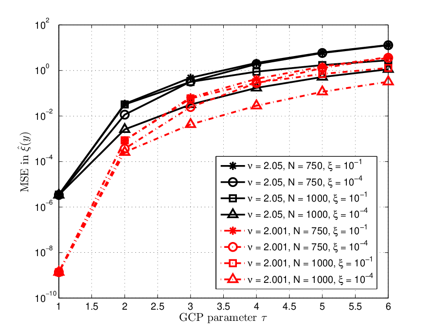
In Fig. 4, we plot the expression in (16). We observe that, in general, the bounds predict an increase in MSE for higher values of τ\tau. Also, for given value of NN, the lower bounds at different signal to noise ratios (SNRs) converge as the value of τ\tau increases, indicating that increasing τ\tau renders the bound insensitive to the SNR. The lower bounds also predict a smaller value of MSE for a lower value of ν\nu.

Refer to caption
Figure 4: Behavior of the MCRB (16) for the parametric form of the GCP, as a function of τ\tau, ν\nu, NN and noise variance ξ\xi.

Thus far, we have presented the lower bounds on the MSE in estimating the unknown parameters of the SBL problem when the noise variance is known. In the next section, we extend the results to the case of unknown noise variance.

IV SMV-SBL: Lower Bounds when σ2\sigma^{2} is Unknown

Let us denote the unknown noise variance as ξ=σ2\xi=\sigma^{2}. In the Bayesian formulation, the noise variance is associated with a prior, and since the IG prior is conjugate to the Gaussian likelihood p𝐘|𝐗,Ξ​(𝐲|𝐱,ξ){p}_{\mathbf{Y}|\mathbf{X},\Xi}(\mathbf{y}|\mathbf{x},\xi), it is assumed that σ2∼ℐ​𝒢​(c,d)\sigma^{2}\sim\mathcal{IG}(c,d) [4], i.e., ξ=σ2\xi=\sigma^{2} is distributed as

pΞ(ξ)≜dcΓ⁡(c)ξ(−c−1)exp{−dξ};ξ∈(0,∞),c,d>0.{p}_{\Xi}(\xi)\triangleq\frac{d^{c}}{\Gamma(c)}\xi^{(-c-1)}\exp\left\{-\frac{d}{\xi}\right\};\quad\xi\in(0,\infty),\penalty\ c,d>0. (18)

Under this assumption, one can marginalize the unknown noise variance and obtain the likelihood p⁡(𝐲|𝐱){p}(\mathbf{y}|\mathbf{x}) as

p⁡(𝐲|𝐱)≜∫ξ=0∞p⁡(𝐲,ξ|𝐱)​𝑑ξ\displaystyle{p}(\mathbf{y}|\mathbf{x})\triangleq\int_{\xi=0}^{\infty}{p}(\mathbf{y},\xi|\mathbf{x})\mathrm{d}\xi
=(2​d)c​Γ​(N2+c)Γ⁡(c)​(π)N/2​((𝐲−𝚽​𝐱)T​(𝐲−𝚽​𝐱)+2​d)−(N2+c),\displaystyle=\frac{(2d)^{c}\Gamma\left(\frac{N}{2}+c\right)}{\Gamma(c)(\pi)^{N/2}}\left((\mathbf{y}-\bm{\Phi}\mathbf{x})^{T}(\mathbf{y}-\bm{\Phi}\mathbf{x})+2d\right)^{-\left(\frac{N}{2}+c\right)}\!, (19)

which is a multivariate Student-tt distribution. It turns out that the straightforward approach of using the above multivariate likelihood to directly compute lower bounds for the various cases given in the previous section is analytically intractable, and that the lower bounds cannot be computed in closed form. Hence, we compute lower bounds from the joint pdf, i.e., we derive the HCRB and BCRBs for the unknown vector 𝜽=[𝐱T,𝜸T,ξ]T\bm{\theta}=[\mathbf{x}^{T},\bm{\gamma}^{T},\xi]^{T} with the MSE matrix 𝐄ξ𝜽\mathbf{E}_{\xi}^{\bm{\theta}} defined by (4).22 2 We use the subscript ξ\xi to indicate that the error matrices and bounds are obtained for the case of unknown noise variance. Using the assumptions and notation from the previous sections, we obtain the following proposition.

Proposition 3

For the signal model in (1), the HCRB on the MSE matrix 𝐄ξ𝛉\mathbf{E}_{\xi}^{\bm{\theta}} of the unknown vector 𝛉=[𝛉′T,ξ]T\bm{\theta}=[{\bm{\theta}^{\prime}}^{T},\xi]^{T}, where 𝛉′=[𝐱T,𝛄T]T\bm{\theta}^{\prime}=[\mathbf{x}^{T},\bm{\gamma}^{T}]^{T}, with the distribution of the compressible vector 𝐱\mathbf{x} given by 𝒩⁡(0,𝚼)\mathcal{N}(0,\bm{\Upsilon}), where 𝛄\bm{\gamma} is modeled as a deterministic or as a random parameter distributed as ∏i=1Lℐ​𝒢​(ν2,ν2​λ)\prod_{i=1}^{L}\mathcal{IG}\left(\frac{\nu}{2},\frac{\nu}{2\lambda}\right), and ξ\xi is modeled as a deterministic parameter, is given by (𝐇ξ𝛉)−1(\mathbf{H}_{\xi}^{\bm{\theta}})^{-1}, where

𝐇ξ𝜽=[𝐇𝜽′𝟎L×1𝟎1×LN2​ξ2].\displaystyle\mathbf{H}_{\xi}^{\bm{\theta}}=\begin{bmatrix}\mathbf{H}^{\bm{\theta}^{\prime}}&\mathbf{0}_{L\times 1}\\ \mathbf{0}_{1\times L}&\frac{N}{2\xi^{2}}\end{bmatrix}. (20)

In the above expression, with a slight abuse of notation, 𝐇𝜽′\mathbf{H}^{\bm{\theta}^{\prime}} is the FIM given by (8) when 𝜸\bm{\gamma} is unknown deterministic and by (10) when 𝜸\bm{\gamma} is random.
Proof: See Appendix -F.
The lower bound on the estimation of ξ\xi matches with known lower bounds on noise variance estimation (see Sec. 3.5 in [19]). One disadvantage of such a bound on ξ^​(𝐲)\hat{\xi}(\mathbf{y}) is that the knowledge of the noise variance is essential to compute the bound, and hence, it cannot be computed offline. Instead, assigning a hyperprior to ξ\xi would result in a lower bound that only depends on the parameters of the hyperprior, which are assumed to be known, allowing the bound to be computed offline. We state the following proposition in this context.

Proposition 4

For the signal model in (1), the HCRB on the MSE matrix 𝐄ξ𝛉\mathbf{E}_{\xi}^{\bm{\theta}} of the unknown vector 𝛉=[𝛉′T,ξ]T\bm{\theta}=[{\bm{\theta}^{\prime}}^{T},\xi]^{T}, where 𝛉′=[𝐱T,𝛄T]T\bm{\theta}^{\prime}=[\mathbf{x}^{T},\bm{\gamma}^{T}]^{T}, with the distribution of the vector 𝐱\mathbf{x} given by 𝒩⁡(0,𝚼)\mathcal{N}(0,\bm{\Upsilon}), where 𝛄\bm{\gamma} is modeled as a deterministic parameter or as a random parameter distributed as ∏i=1Lℐ​𝒢​(ν2,ν2​λ)\prod_{i=1}^{L}\mathcal{IG}\left(\frac{\nu}{2},\frac{\nu}{2\lambda}\right), and with the random parameter ξ\xi distributed as ℐ​𝒢​(c,d)\mathcal{IG}(c,d), is given by (𝐇ξ𝛉)−1(\mathbf{H}_{\xi}^{\bm{\theta}})^{-1}, where

𝐇ξ𝜽=[𝐇𝜽′𝟎L×1𝟎1×Lc⁡(c+1)​(N/2+c+3)d2].\displaystyle\mathbf{H}_{\xi}^{\bm{\theta}}=\begin{bmatrix}\mathbf{H}^{\bm{\theta}^{\prime}}&\mathbf{0}_{L\times 1}\\ \mathbf{0}_{1\times L}&\frac{c(c+1)(N/2+c+3)}{d^{2}}\end{bmatrix}. (21)

In (21), 𝐇𝜽′\mathbf{H}^{\bm{\theta}^{\prime}} is the FIM given in (8) when 𝜸\bm{\gamma} is unknown deterministic and by (10) when 𝜸\bm{\gamma} is random.
Proof: See Appendix -G.

In SBL problems, a non-informative prior on ξ\xi is typically preferred, i.e., the distribution of the noise variance is modeled to be as flat as possible. In [4], it was observed that a non-informative prior is obtained when c,d→0c,d\rightarrow 0. However, as c,d→0c,d\rightarrow 0, the bound in (21) is indeterminate. In Sec. VI, we illustrate the performance of the lower bound in (21) for practical values of cc and dd.

IV-A Marginalized Bounds

In this subsection, we obtain lower bounds on the MSE of the estimator ξ^​(𝐲)\hat{\xi}(\mathbf{y}), in the presence of nuisance variables in the joint distribution. To start with, we consider the marginalized distributions of 𝜸\bm{\gamma} and ξ\xi, i.e., p𝐘;𝜸,ξ​(𝐲,𝜸,ξ){p}_{\mathbf{Y};\bm{\gamma},\xi}(\mathbf{y};\bm{\gamma},\xi) where both, 𝜸\bm{\gamma} and ξ\xi are deterministic variables. Since the unknowns are deterministic, the regularity condition has to be satisfied for 𝜽=[𝜸T,ξ]T\bm{\theta}=[\bm{\gamma}^{T},\xi]^{T}. We state the following theorem.

Theorem 4

For the signal model in (1), the log likelihood function log⁡p𝐘;𝛄,ξ​(𝐲,𝛄,ξ)\log{p}_{\mathbf{Y};\bm{\gamma},\xi}(\mathbf{y};\bm{\gamma},\xi) satisfies the regularity condition [19]. Further, the MCRB on the MSE matrix 𝐄ξ𝛉\mathbf{E}_{\xi}^{\bm{\theta}} of the unknown deterministic vector 𝛉=[𝛄T,ξ]T\bm{\theta}=[\bm{\gamma}^{T},\xi]^{T} is given by 𝐄ξ𝛉⪰(𝐌ξ𝛉)−1\mathbf{E}_{\xi}^{\bm{\theta}}\succeq({\mathbf{M}_{\xi}^{\bm{\theta}}})^{-1}, where

𝐌ξ𝜽≜[𝐌ξ𝜽​(𝜸)𝐌ξ𝜽​(𝜸,ξ)𝐌ξ𝜽​(ξ,𝜸)𝐌ξ𝜽​(ξ)],\mathbf{M_{\xi}^{\bm{\theta}}}\triangleq\begin{bmatrix}\mathbf{M}_{\xi}^{\bm{\theta}}(\bm{\gamma})&\mathbf{M}_{\xi}^{\bm{\theta}}(\bm{\gamma},\xi)\\ \mathbf{M}_{\xi}^{\bm{\theta}}(\xi,\bm{\gamma})&\mathbf{M}_{\xi}^{\bm{\theta}}(\xi)\end{bmatrix}, (22)

where the (i​j)th(ij)^{\text{th}} entry of the matrix 𝐌ξ𝛉​(𝛄)\mathbf{M_{\xi}^{\bm{\theta}}}(\bm{\gamma}) is given by (𝐌ξ𝛉​(𝛄))i​j=12​{(ΦjT​𝚺y−1​Φi)2}(\mathbf{M_{\xi}^{\bm{\theta}}}(\bm{\gamma}))_{ij}=\frac{1}{2}\left\{(\Phi_{j}^{T}\bm{\Sigma}_{y}^{-1}\Phi_{i})^{2}\right\}, and 𝐌ξ𝛉​(ξ)=12​Tr​(𝚺y−2)\mathbf{M^{\bm{\theta}}_{\xi}}(\xi)=\frac{1}{2}\mbox{Tr}(\bm{\Sigma}_{y}^{-2}). Further, (𝐌ξ𝛉​(𝛄,ξ))i=(𝐌ξ𝛉​(ξ,𝛄))i=ΦiT​𝚺y−2​Φi2(\mathbf{M}_{\xi}^{\bm{\theta}}(\bm{\gamma},\xi))_{i}=(\mathbf{M}_{\xi}^{\bm{\theta}}(\xi,\bm{\gamma}))_{i}=\frac{\Phi_{i}^{T}\bm{\Sigma}_{y}^{-2}\Phi_{i}}{2}, i,j=1,2,…,Li,j=1,2,\ldots,L.

Proof: See Appendix -H.

Remark: From the graphical model in Fig. 1, it can be seen that the branches consisting of γi\gamma_{i} and ξ\xi are independent conditioned on 𝐱\mathbf{x}. However, when 𝐱\mathbf{x} is marginalized, the nodes ξ\xi and γi\gamma_{i} are connected, and hence, Lemma 1 is no longer valid. Due to this, the lower bound on 𝜸\bm{\gamma} depends on ξ\xi and vice versa, i.e., 𝐌ξ𝜽​(𝜸)\mathbf{M_{\xi}^{\bm{\theta}}(\bm{\gamma})} and 𝐌ξ𝜽​(ξ)\mathbf{M_{\xi}^{\bm{\theta}}(\xi)} depend on both ξ\xi and 𝚼=diag​(𝜸)\bm{\Upsilon}=\mbox{diag}(\bm{\gamma}) through 𝚺y=ξ​𝐈N×N+𝚽​𝚼​𝚽T\bm{\Sigma}_{y}=\xi\mathbf{I}_{N\times N}+\bm{\Phi}\bm{\Upsilon}\bm{\Phi}^{T}.

Thus far, we have presented several bounds for the MSE performance of the estimators 𝐱^​(𝐲)\hat{\mathbf{x}}(\mathbf{y}), 𝜸^​(𝐲)\hat{\bm{\gamma}}(\mathbf{y}) and ξ^​(𝐲)\hat{\xi}(\mathbf{y}) in the SMV-SBL framework. In the next section, we derive Cramér-Rao type lower bounds for the MMV-SBL signal model.

V Lower Bounds for the MMV-SBL

In this section, we provide Cramér-Rao type lower bounds for the estimation of unknown parameters in the MMV-SBL model given in (2). We consider the estimation of the compressible vector 𝐰\mathbf{w} from the vector of observations 𝐭\mathbf{t}, which contain the stacked columns of 𝐖\mathbf{W} and 𝐓\mathbf{T}, respectively. In the MMV-SBL model, each column of 𝐖\mathbf{W} is distributed as 𝐰i∼𝒩⁡(0,𝚼)\mathbf{w}_{i}\sim\mathcal{N}(0,\bm{\Upsilon}), for i=1,…​Mi=1,\ldots M, and the likelihood is given by ∏i=1Mp𝐓|𝐖i,Ξ​(𝐭i|𝐰i,ξ)\prod_{i=1}^{M}{p}_{\mathbf{T}|\mathbf{W}_{i},\Xi}(\mathbf{t}_{i}|\mathbf{w}_{i},\xi), where p𝐓|𝐖i​Ξ​(𝐭i|𝐰i,ξ)=𝒩⁡(𝚽​𝐰i,ξ){p}_{\mathbf{T}|\mathbf{W}_{i}\Xi}(\mathbf{t}_{i}|\mathbf{w}_{i},\xi)=\mathcal{N}(\bm{\Phi}\mathbf{w}_{i},\xi) and ξ=σ2\xi=\sigma^{2}. The modeling assumptions on 𝜸\bm{\gamma} and ξ\xi are the same as in the SMV-SBL case, given by (9) and (18), respectively [18].

Using the notation developed in Sec. II, we derive the bounds for the MMV SBL case similar to the SMV-SBL cases considered in Secs. III and IV. Since the derivation of these bounds follow along the same lines as in the previous sections, we simply state results in Table I.

Bound Derived Expression
HCRB on 𝜸^​(𝐲)\hat{\bm{\gamma}}(\mathbf{y}) 𝐇M𝜽=diag​(M2​γi2)\mathbf{H}_{M}^{\bm{\theta}}=\mbox{diag}\left(\frac{M}{2\gamma_{i}^{2}}\right), i=1,2​…,Li=1,2\ldots,L
BCRB on 𝜸^​(𝐲)\hat{\bm{\gamma}}(\mathbf{y}) 𝐁M𝜽=λ2​(ν+2)​(M+ν+6)2​ν​𝐈L×L\mathbf{B}_{M}^{\bm{\theta}}=\frac{\lambda^{2}(\nu+2)(M+\nu+6)}{2\nu}\mathbf{I}_{L\times L}
MCRB on 𝜸^​(𝐲)\hat{\bm{\gamma}}(\mathbf{y}) 𝐌M𝜽=[𝐌i​j𝜽]\mathbf{M}_{M}^{\bm{\theta}}=[\mathbf{M}_{ij}^{\bm{\theta}}],
where 𝐌i​j𝜽=M2​(ΦjT​𝚺y−1​Φi)2\mathbf{M}_{ij}^{\bm{\theta}}=\frac{M}{2}(\Phi_{j}^{T}\bm{\Sigma}_{y}^{-1}\Phi_{i})^{2}
HCRB on 𝐰^​(𝐲)\hat{\mathbf{w}}(\mathbf{y}) 𝐇M𝜽=(𝚽T​𝚽σ2+𝚼−1)⊗𝐈M×M\mathbf{H}_{M}^{\bm{\theta}}=\left(\frac{\bm{\Phi}^{T}\bm{\Phi}}{\sigma^{2}}+{\bm{\Upsilon}^{-1}}\right)\otimes\mathbf{I}_{M\times M}
BCRB on 𝐰^​(𝐲)\hat{\mathbf{w}}(\mathbf{y}) 𝐁M𝜽=(𝚽T​𝚽σ2+λ​𝐈L×L)⊗𝐈M×M\mathbf{B}_{M}^{\bm{\theta}}=\left(\frac{\bm{\Phi}^{T}\bm{\Phi}}{\sigma^{2}}+{\lambda}\mathbf{I}_{L\times L}\right)\otimes\mathbf{I}_{M\times M}
HCRB on ξ^​(𝐲)\hat{\xi}(\mathbf{y}) 𝐇M,ξ𝜽=(M​N2​ξ2)\mathbf{H}_{M,\xi}^{\bm{\theta}}=\left(\frac{MN}{2\xi^{2}}\right)
BCRB on ξ^​(𝐲)\hat{\xi}(\mathbf{y}) 𝐁M,ξ𝜽=c​(M​N2+c+3)​(c+1)d2\mathbf{B}_{M,\xi}^{\bm{\theta}}=\frac{c\left(\frac{MN}{2}+c+3\right)(c+1)}{d^{2}}
MCRB on [𝜸^(𝐲)T[\hat{\bm{\gamma}}(\mathbf{y})^{T}, ξ^(𝐲)]T\hat{\xi}(\mathbf{y})]^{T} 𝐌M,ξ𝜽=M×𝐌ξ𝜽\mathbf{M}_{M,\xi}^{\bm{\theta}}={M}\times\mathbf{M_{\xi}^{\bm{\theta}}}
Table I: Cramér-Rao Type Bounds for the MMV-SBL Case.

We see that the lower bounds on 𝜸^​(𝐲)\hat{\bm{\gamma}}(\mathbf{y}) and ξ^​(𝐲)\hat{\xi}(\mathbf{y}) are reduced by a factor of MM compared to the SMV case, which is intuitively satisfying. It turns out that it is not possible to obtain the MCRB on 𝐰\mathbf{w} in the MMV-SBL setting, since closed form expressions for the FIM are not available.

In the next section, we consider two popular algorithms for SBL and graphically illustrate the utility of the lower bounds.

VI Simulations and Discussion

The vector estimation problem in the SBL framework typically involves the joint estimation of the hyperparameter and the unknown compressible vector 𝐱\mathbf{x}. Since the hyperparameter estimation problem cannot be solved in closed form, iterative estimators are employed [4]. In this section, we consider the iterative updates based on the EM algorithm first proposed in [4]. We also consider the algorithm proposed in [6] based on the Automatic Relevance Determination (ARD) framework. We plot the MSE performance in estimating 𝐱\mathbf{x}, 𝜸\bm{\gamma} and ξ\xi with the linear model in (1) and (2), for the EM algorithm, labeled EM, and the ARD based Reweighted ℓ1\ell_{1} algorithm, labeled ARD-SBL. We compare the performance of the estimators against the derived lower bounds.

Refer to caption
Figure 5: Decay profile of the sorted magnitudes of i.i.d. samples drawn from a Student-tt distribution.

We simulate the lower bounds for a random underdetermined (N<LN<L) measurement matrix 𝚽\bm{\Phi}, whose entries are i.i.d. and standard Bernoulli ({+1,−1})\left(\left\{+1,-1\right\}\right) distributed. A compressible signal of dimension LL is generated by sampling from a Student-tt distribution with the value of ν\nu ranging from 2.012.01 to 2.052.05, which is the range in which the signal is “somewhat” compressible, for high dimensional signals [3]. Figure 5 shows the decay profile of the sorted magnitudes of L=1024L=1024 i.i.d. samples drawn from a Student-tt distribution for different ν\nu and with the value of 𝔼⁡(xi2)\mathbb{E}(x_{i}^{2}) fixed at 10−310^{-3}.

VI-A Lower Bounds on the MSE Performance of 𝐱^​(𝐲)\hat{\mathbf{x}}(\mathbf{y})

Refer to caption
Figure 6: The MSE performance of 𝐱^​(𝐲)\hat{\mathbf{x}}(\mathbf{y}) and the corresponding MCRB and BCRB, as a function of SNR, with ν=2.01\nu=2.01.

In this subsection, we compare the MSE performance of the ARD-SBL estimator and the EM based estimator 𝐱^​(𝐲)\hat{\mathbf{x}}(\mathbf{y}). Figure 6 depicts the MSE performance of 𝐱^​(𝐲)\hat{\mathbf{x}}(\mathbf{y}) for different SNRs and N=750N=750 and 10001000, with ν=2.01\nu=2.01. We compare it with the HCRB/BCRB derived in (8), which is obtained by assuming the knowledge of the realization of the hyperparameters 𝜸\bm{\gamma}. We see that the MCRB derived in (14) is a tight lower bound on the MSE performance at high SNR and NN.

Refer to caption
Figure 7: The MSE performance of 𝐱^​(𝐲)\hat{\mathbf{x}}(\mathbf{y}) and the corresponding MCRB and BCRB, as a function of ν\nu, with SNR = 4040 dB.
Refer to caption
Figure 8: The MSE performance of 𝐱^​(𝐲)\hat{\mathbf{x}}(\mathbf{y}) and the corresponding MCRB and BCRB, as a function of NN, with SNR = 4040 dB.

Figure 7 shows the comparative MSE performance of the ARD-SBL estimator and EM based estimator as a function of varying degrees of freedom ν\nu, at an SNR of 4040 dB and N=1000N=1000 and 750750. As expected, the MSE performance of the algorithms is better at low values of ν\nu since the signal is more compressible, and the MCRB and BCRB also reflect this behavior. The MCRB is a tight lower bound, especially for high values of NN. Figure 8 shows the MSE performance of the ARD-SBL estimator and EM based estimator as a function of NN, at an SNR of 4040 dB and for two different values of ν\nu. The MSE performance of the EM algorithm converges to that of the MCRB at higher NN.

VI-B Lower Bounds on the MSE Performance of 𝛄^​(𝐲)\hat{\bm{\gamma}}(\mathbf{y})

In this subsection, we compare the different lower bounds for the MSE of the estimator 𝜸^​(𝐲)\hat{\bm{\gamma}}(\mathbf{y}) for the SMV and MMV-SBL system model. Figure 9 shows the MSE performance of 𝜸^​(𝐲)\hat{\bm{\gamma}}(\mathbf{y}) as a function of SNR and MM, when γ\gamma is a random parameter, N=1000N=1000 and ν=2.01\nu=2.01. In this case, it turns out that there is a large gap between the performance of the EM based estimate and the lower bound.

Refer to caption
Figure 9: The MSE performance of 𝜸^​(𝐲)\hat{\bm{\gamma}}(\mathbf{y}) and the corresponding HCRB, as a function of SNR, with N=1000N=1000.

When 𝜸\bm{\gamma} is deterministic, we first note that the EM based ML estimator for 𝜸\bm{\gamma} is asymptotically optimal and the lower bounds are practical for large data samples [19]. The results are listed in Table II. We see that for L=2048L=2048 and N=1500N=1500, the MCRB and BCRB are tight lower bounds, with MCRB being marginally tighter than the BCRB. However, as MM increases, the gap between the MSE and the lower bounds increases.

SNR(dB) 1010 2020 3030 4040
M=1M=1 MSE 0.0540.054 0.0530.053 0.0510.051 0.0500.050
MCRB 0.0520.052 0.0510.051 0.0500.050 0.0490.049
BCRB 0.0490.049 0.0490.049 0.0490.049 0.0490.049
M=50M=50 MSE 0.04500.0450 0.0390.039 0.0350.035 0.0300.030
MCRB ×10−2\times 10^{-2} 0.120.12 0.110.11 0.100.10 0.090.09
BCRB×10−3\times 10^{-3} 0.9770.977 0.9770.977 0.9770.977 0.9770.977
Table II: Values of the MSE of the estimator 𝜸^​(𝐲)\hat{\bm{\gamma}}(\mathbf{y}), the MCRB and the BCRB, for 𝜽d=[𝜸]\bm{\theta}_{d}=[\bm{\gamma}] as a function of SNR, for N=1500N=1500.

VI-C Lower Bounds on the MSE Performance of ξ^​(𝐲)\hat{\xi}(\mathbf{y})

In Fig. 10, we compare the lower bounds on the MSE of the estimator ξ^​(𝐲)\hat{\xi}(\mathbf{y}) in the SMV and MMV-SBL settings, for different values of NN and MM. Here, ξ\xi is sampled from the IG pdf (18), with parameters c=3c=3 and d=0.2d=0.2.

Refer to caption
Figure 10: The MSE performance of ξ^​(𝐲)\hat{\xi}(\mathbf{y}) and its HCRB, as a function of NN.

When ξ\xi is deterministic, the EM based ML estimator for 𝜸\bm{\gamma} is asymptotically optimal and the lower bounds are practical for large data samples [19]. Table III lists the MSE values of ξ^​(𝐲)\hat{\xi}(\mathbf{y}), the corresponding HCRB and MCRB for deterministic but unknown noise variance, while the true noise variance is fixed at 10−310^{-3}. We see that for L=2048L=2048 and N=1500N=1500, the MCRB is marginally tighter than the HCRB. However, when the noise variance is random, we see from Fig. 10 that there is a large gap between the MSE performance and the HCRB.

NN 15001500 16001600 17001700 18001800
M=1M=1 MSE ×10−8\times 10^{-8} 0.7360.736 0.6630.663 0.6360.636 0.5920.592
MCRB×10−8\times 10^{-8} 0.3800.380 0.3400.340 0.3070.307 0.2790.279
HCRB×10−8\times 10^{-8} 0.1330.133 0.1250.125 0.1180.118 0.1110.111
M=50M=50 MSE ×10−9\times 10^{-9} 0.9300.930 0.8920.892 0.8660.866 0.8470.847
MCRB×10−10\times 10^{-10} 0.6800.680 0.6520.652 0.6140.614 0.5730.573
HCRB×10−10\times 10^{-10} 0.2670.267 0.2500.250 0.2350.235 0.2220.222
Table III: Values of the MSE of the estimator ξ^​(𝐲)\hat{\xi}(\mathbf{y}), the MCRB and the HCRB for θd=[ξ]\theta_{d}=[\xi], as a function of NN.

VII Conclusion

In this work, we derived Cramér-Rao type lower bounds on the MSE, namely, the HCRB, BCRB and MCRB, for the SMV-SBL and the MMV-SBL problem of estimating compressible signals. We used a hierarchical model for the compressible priors to obtain the bounds under various assumptions on the unknown parameters. The bounds derived by assuming a hyperprior distribution on the hyperparameters themselves provided key insights into the MSE performance of SBL and the values of the parameters that govern these hyperpriors. We derived the MCRB for the generalized compressible prior distribution, of which the Student-tt and Generalized Pareto prior distribution are special cases. We showed that the MCRB is tighter than the BCRB. We compared the lower bounds with the MSE performance of the ARD-SBL and the EM algorithm using Monte Carlo simulations. The numerical results illustrated the near-optimality of EM based updates for SBL, which makes it attractive for practical implementations.

-A Proof of Proposition 1

Using the graphical model of Fig. 1 in (5),

𝐇𝜽​(𝐱)\displaystyle\mathbf{H}^{\bm{\theta}}(\mathbf{x}) ≜\displaystyle\triangleq −𝔼𝐘,𝐗;𝜸​[∇𝐱2​log⁡p𝐘,𝐗;𝜸​(𝐲,𝐱,𝜸)]\displaystyle-\mathbb{E}_{\mathbf{Y},\mathbf{X};\bm{\gamma}}\left[\nabla_{\mathbf{x}}^{2}\log{p}_{\mathbf{Y},\mathbf{X};\bm{\gamma}}(\mathbf{y},\mathbf{x};\bm{\gamma})\right] (23)
=\displaystyle= −𝔼𝐘,𝐗;𝜸​[∇𝐱(𝚽T​(𝐲−𝚽​𝐱)σ2−𝚼−1​𝐱)]\displaystyle-\mathbb{E}_{\mathbf{Y},\mathbf{X};\bm{\gamma}}\left[\nabla_{\mathbf{x}}\left(\frac{\bm{\Phi}^{T}(\mathbf{y}-\bm{\Phi}\mathbf{x})}{\sigma^{2}}-{\bm{\Upsilon}^{-1}\mathbf{x}}\right)\right]
=\displaystyle= 𝚽T​𝚽σ2+𝚼−1.\displaystyle\frac{\bm{\Phi}^{T}\bm{\Phi}}{\sigma^{2}}+\bm{\Upsilon}^{-1}.

Similarly, it is straightforward to show that ∇𝐱∇𝜸​log⁡p𝐘,𝐗;𝜸​(𝐲,𝐱,𝜸)=diag​(x1γ12,x2γ22,…,xLγL2)\nabla_{\mathbf{x}}\nabla_{\bm{\gamma}}\log{p}_{\mathbf{Y},\mathbf{X};\bm{\gamma}}(\mathbf{y},\mathbf{x};\bm{\gamma})=\textnormal{diag}\left(\frac{x_{1}}{\gamma_{1}^{2}},\penalty\ \frac{x_{2}}{\gamma_{2}^{2}},\penalty\ \ldots,\penalty\ \frac{x_{L}}{\gamma_{L}^{2}}\right). Since xix_{i} are zero mean random variables,

𝐇𝜽​(𝜸,𝐱)=−𝔼𝐘,𝐗;𝜸​[∇𝜸∇𝐱​log⁡p𝐘,𝐗;𝜸​(𝐲,𝐱,𝜸)]=𝟎L×L,\displaystyle\mathbf{H}^{\bm{\theta}}(\bm{\gamma},\mathbf{x})=-\mathbb{E}_{\mathbf{Y},\mathbf{X};\bm{\gamma}}\left[\nabla_{\bm{\gamma}}\nabla_{\mathbf{x}}\log{p}_{\mathbf{Y},\mathbf{X};\bm{\gamma}}(\mathbf{y},\mathbf{x};\bm{\gamma})\right]=\mathbf{0}_{L\times L},
𝐇𝜽​(𝜸)=−𝔼𝐘,𝐗;𝜸​[∇𝜸2(log⁡p𝐘|𝐗​(𝐲|𝐱)+log⁡p𝐗;𝜸​(𝐱,𝜸))].\mathbf{H}^{\bm{\theta}}(\bm{\gamma})=-\mathbb{E}_{\mathbf{Y},\mathbf{X};\bm{\gamma}}\left[\nabla_{\bm{\gamma}}^{2}(\log{p}_{\mathbf{Y}|\mathbf{X}}(\mathbf{y}|\mathbf{x})+\log{p}_{\mathbf{X};\bm{\gamma}}(\mathbf{x};\bm{\gamma}))\right].

Now, since log⁡p𝐗;𝜸​(𝐱,𝜸)=∑i=1Llog⁡p𝐗;𝜸​(𝐱i,𝜸i)\log{p}_{\mathbf{X};\bm{\gamma}}(\mathbf{x};\bm{\gamma})=\sum_{i=1}^{L}\log{p}_{\mathbf{X};\bm{\gamma}}(\mathbf{x}_{i};\bm{\gamma}_{i}), we get,

∂2log⁡p𝐗;𝜸​(𝐱,𝜸)∂γi​∂γj\displaystyle\frac{\partial^{2}\log{p}_{\mathbf{X};\bm{\gamma}}(\mathbf{x};\bm{\gamma})}{\partial\gamma_{i}\partial\gamma_{j}} =\displaystyle= {12​γi2−xi2γi3if​i=j0if​i≠j.\displaystyle\left\{\begin{array}[]{ll}\frac{1}{2\gamma_{i}^{2}}-\frac{x_{i}^{2}}{\gamma_{i}^{3}}&\mbox{if}\penalty\ i=j\\ 0&\mbox{if}\penalty\ i\neq j.\end{array}\right.

Taking −𝔼𝐗;𝜸​(⋅)-\mathbb{E}_{\mathbf{X};\bm{\gamma}}(\cdot) on both sides of the above equation and noting that 𝔼𝐗;𝜸​(xi2)=γi\mathbb{E}_{\mathbf{X};\bm{\gamma}}(x_{i}^{2})=\gamma_{i}, we obtain

𝐇𝜽​(𝜸)\displaystyle\mathbf{H}^{\bm{\theta}}(\bm{\gamma}) =\displaystyle= diag​(−𝔼𝐗;𝜸​[∂2log⁡p𝐗;𝜸​(𝐱,𝜸)∂γi2])\displaystyle\mbox{diag}\left(-\mathbb{E}_{\mathbf{X};\bm{\gamma}}\left[\frac{\partial^{2}\log{p}_{\mathbf{X};\bm{\gamma}}(\mathbf{x};\bm{\gamma})}{\partial\gamma_{i}^{2}}\right]\right) (27)
=\displaystyle= diag​([12​γ12,…,12​γL2]).\displaystyle\mbox{diag}\left(\left[\frac{1}{2\gamma_{1}^{2}},\ldots,\frac{1}{2\gamma_{L}^{2}}\right]\right).

This completes the proof.

-B Proof of Proposition 2

Using the graphical model of Fig. 1 in (5),

𝐁𝜽​(𝐱)\displaystyle\mathbf{B}^{\bm{\theta}}(\mathbf{x}) ≜\displaystyle\triangleq −𝔼𝐘,𝐗,Γ​[∇𝐱2​log⁡p𝐘,𝐗,Γ​(𝐲,𝐱,𝜸)]\displaystyle-\mathbb{E}_{\mathbf{Y},\mathbf{X},\Gamma}\left[\nabla_{\mathbf{x}}^{2}\log{p}_{\mathbf{Y},\mathbf{X},\Gamma}(\mathbf{y},\mathbf{x};\bm{\gamma})\right] (28)
=\displaystyle= −𝔼𝐘,𝐗,Γ​[∇𝐱(𝚽T​(𝐲−𝚽​𝐱)σ2−𝚼−1​𝐱)]\displaystyle-\mathbb{E}_{\mathbf{Y},\mathbf{X},\Gamma}\left[\nabla_{\mathbf{x}}\left(\frac{\bm{\Phi}^{T}(\mathbf{y}-\bm{\Phi}\mathbf{x})}{\sigma^{2}}-{\bm{\Upsilon}^{-1}\mathbf{x}}\right)\right]
=\displaystyle= 𝔼Γ​[𝚽T​𝚽σ2+𝚼−1]\displaystyle\mathbb{E}_{\Gamma}\left[\frac{\bm{\Phi}^{T}\bm{\Phi}}{\sigma^{2}}+\bm{\Upsilon}^{-1}\right]
=\displaystyle= 𝚽T​𝚽σ2+𝔼Γ​[𝚼−1].\displaystyle\frac{\bm{\Phi}^{T}\bm{\Phi}}{\sigma^{2}}+\mathbb{E}_{\Gamma}\left[\bm{\Upsilon}^{-1}\right]. (29)

The expression for 𝔼Γ​[𝚼−1]\mathbb{E}_{\Gamma}\left[\bm{\Upsilon}^{-1}\right] w.r.t. γi\gamma_{i} is given by,

𝔼Γ​[1γi]\displaystyle\mathbb{E}_{\Gamma}\left[\frac{1}{\gamma_{i}}\right] =\displaystyle= Kγ​∫γi=0∞γi(−ν2−2)​exp⁡{−ν2​λ​γi}​d​γi\displaystyle K_{\gamma}\int_{\gamma_{i}=0}^{\infty}\gamma_{i}^{\left(-\frac{\nu}{2}-2\right)}\exp\left\{-\frac{\nu}{2\lambda\gamma_{i}}\right\}\mathrm{d}\gamma_{i} (30)
=\displaystyle= Kγ​Γ⁡(ν2+1)(ν2​λ)ν2+1​∫γi=0∞ℐ​𝒢​(ν2+1,ν2​λ)​d​γi⏟=1\displaystyle K_{\gamma}\frac{\Gamma\left(\frac{\nu}{2}+1\right)}{\left(\frac{\nu}{2\lambda}\right)^{\frac{\nu}{2}+1}}\underbrace{\int_{\gamma_{i}=0}^{\infty}\mathcal{IG}\left(\frac{\nu}{2}+1,\frac{\nu}{2\lambda}\right)\mathrm{d}\gamma_{i}}_{=1}
=\displaystyle= λ,\displaystyle\lambda, (31)

since Kγ=(ν2​λ)ν/2​(Γ⁡(ν2))−1K_{\gamma}=\left(\frac{\nu}{2\lambda}\right)^{\nu/2}\left(\Gamma\left(\frac{\nu}{2}\right)\right)^{-1}. Hence, the overall bound is given by

𝐁𝜽​(𝐱)=𝚽T​𝚽σ2+λ​𝐈L×L.\mathbf{B}^{\bm{\theta}}(\mathbf{x})=\frac{\bm{\Phi}^{T}\bm{\Phi}}{\sigma^{2}}+\lambda\mathbf{I}_{L\times L}. (32)

Using the graphical model of Fig. 1 in (5), for 𝜽=[𝐱T,𝜸T]T\bm{\theta}=[\mathbf{x}^{T},\bm{\gamma}^{T}]^{T}, 𝐁𝜽​(𝜸)\mathbf{B}^{\bm{\theta}}(\bm{\gamma}) is defined as

𝐁𝜽(𝜸)≜−𝔼𝐘,𝐗,Γ[∇𝜸2(logp𝐘|𝐗(𝐲|𝐱)\displaystyle\mathbf{B}^{\bm{\theta}}(\bm{\gamma})\triangleq-\mathbb{E}_{\mathbf{Y},\mathbf{X},\Gamma}\left[\nabla_{\bm{\gamma}}^{2}\left(\log{p}_{\mathbf{Y}|\mathbf{X}}(\mathbf{y}|\mathbf{x})\right.\right.
+logp𝐗|Γ(𝐱|𝜸)+logpΓ(𝜸))].\displaystyle\left.\left.+\log{p}_{\mathbf{X}|\Gamma}(\mathbf{x}|\bm{\gamma})+\log{p}_{\Gamma}(\bm{\gamma})\right)\right]. (33)

Since the expressions for log⁡p𝐗|Γ​(𝐱|𝜸)\log{p}_{\mathbf{X}|\Gamma}(\mathbf{x}|\bm{\gamma}) and log⁡pΓ​(𝜸)\log{p}_{\Gamma}(\bm{\gamma}) are separable and symmetric w.r.t. γi\gamma_{i}, the off-diagonal terms of 𝐁𝜽​(𝜸)\mathbf{B}^{\bm{\theta}}(\bm{\gamma}) are zero, and it is sufficient to evaluate the diagonal terms −𝔼𝐘,𝐗,Γ​(∂2(log⁡p𝐗|Γ​(𝐱|𝜸)+log⁡pΓ​(𝜸))∂γi2)-\mathbb{E}_{\mathbf{Y},\mathbf{X},\Gamma}\left(\frac{\partial^{2}(\log{p}_{\mathbf{X}|\Gamma}(\mathbf{x}|\bm{\gamma})+\log{p}_{\Gamma}(\bm{\gamma}))}{\partial\gamma_{i}^{2}}\right). Differentiating the expression w.r.t. γi\gamma_{i} twice,

∂2(log⁡p𝐗|Γ​(𝐱|𝜸)+log⁡pΓ​(𝜸))∂γi2=−(ν+1)2​γi2+νλ​γi3.\frac{\partial^{2}\left(\log{p}_{\mathbf{X}|\Gamma}(\mathbf{x}|\bm{\gamma})+\log{p}_{\Gamma}(\bm{\gamma})\right)}{\partial\gamma_{i}^{2}}=-\frac{(\nu+1)}{2\gamma_{i}^{2}}+\frac{\nu}{\lambda\gamma_{i}^{3}}. (34)

The expression for −𝔼Γ​[−(ν+1)2​γi2+νλ​γi3]-\mathbb{E}_{\Gamma}\left[-\frac{(\nu+1)}{2\gamma_{i}^{2}}+\frac{\nu}{\lambda\gamma_{i}^{3}}\right] is given by

𝔼Γ​[(ν+1)2​γi2−νλ​γi3]=Kγ\displaystyle\mathbb{E}_{\Gamma}\left[\frac{(\nu+1)}{2\gamma_{i}^{2}}-\frac{\nu}{\lambda\gamma_{i}^{3}}\right]=K_{\gamma}
∫γi=0∞[(ν+1)​γi−22−ν​γi−3λ]​γi(−ν2−1)​exp⁡{−ν2​λ​γi}​d​γi,\displaystyle\int\limits_{\gamma_{i}=0}^{\infty}\left[\frac{(\nu+1){\gamma_{i}^{-2}}}{2}-\frac{\nu{\gamma_{i}^{-3}}}{\lambda}\right]\gamma_{i}^{\left(-\frac{\nu}{2}-1\right)}\exp\{-\frac{\nu}{2\lambda\gamma_{i}}\}\mathrm{d}\gamma_{i}, (35)

where Kγ=(ν2​λ)ν/2​(Γ⁡(ν2))−1K_{\gamma}=\left(\frac{\nu}{2\lambda}\right)^{\nu/2}\left(\Gamma\left(\frac{\nu}{2}\right)\right)^{-1}. After some manipulation, it can be shown that the above integral reduces to

−𝔼Γ​[−(ν+1)2​γi2+νλ​γi3]=λ2​(ν+2)​(ν+7)2​ν.-\mathbb{E}_{\Gamma}\left[-\frac{(\nu+1)}{2\gamma_{i}^{2}}+\frac{\nu}{\lambda\gamma_{i}^{3}}\right]=\frac{\lambda^{2}(\nu+2)(\nu+7)}{2\nu}. (36)

Thus, the (i​j)th(ij)^{\text{th}} component of 𝐁𝜽​(𝜸,𝐱)\mathbf{B}^{\bm{\theta}}(\bm{\gamma},\mathbf{x}) is given by

(𝐁𝜽​(𝜸,𝐱))i​j=∂2log⁡p𝐗|Γ​(𝐱|𝜸)∂γi​∂xi=−xiγi2,(\mathbf{B}^{\bm{\theta}}(\bm{\gamma},\mathbf{x}))_{ij}=\frac{\partial^{2}\log{p}_{\mathbf{X}|\Gamma}(\mathbf{x}|\bm{\gamma})}{\partial\gamma_{i}\partial x_{i}}=-\frac{x_{i}}{\gamma_{i}^{2}}, (37)

and 𝐁𝜽​(𝐱,𝜸)=(𝐁𝜽​(𝜸,𝐱))T\mathbf{B}^{\bm{\theta}}(\mathbf{x},\bm{\gamma})=(\mathbf{B}^{\bm{\theta}}(\bm{\gamma},\mathbf{x}))^{T}. Since 𝔼𝐗|Γ​(xi)=0\mathbb{E}_{\mathbf{X}|\Gamma}(x_{i})=0, 𝐁𝜽​(𝜸,𝐱)=𝟎L×L\mathbf{B}^{\bm{\theta}}(\bm{\gamma},\mathbf{x})=\mathbf{0}_{L\times L}. This completes the proof.

-C Proof of Theorem 1

To establish the regularity condition, the first order derivative of the log likelihood log⁡p𝐘;𝜸​(𝐲,𝜸)\log{p}_{\mathbf{Y};\bm{\gamma}}(\mathbf{y};\bm{\gamma}) is required. This, in turn, requires the evaluation of ∂log⁡|𝚺y|∂γj\frac{\partial\log|\bm{\Sigma}_{y}|}{\partial\gamma_{j}} and ∂𝐲T​𝚺y−1​𝐲∂γj\frac{\partial\mathbf{y}^{T}\bm{\Sigma}_{y}^{-1}\mathbf{y}}{\partial\gamma_{j}}. Using the chain rule for differentiation [26], we have

∂log⁡|𝚺y|∂γj\displaystyle\frac{\partial\log|\bm{\Sigma}_{y}|}{\partial\gamma_{j}} =Tr​{(∂log⁡|𝚺y|∂𝚺y)T​∂𝚺y∂γj}\displaystyle=\mbox{Tr}\left\{\left(\frac{\partial\log|\bm{\Sigma}_{y}|}{\partial\bm{\Sigma}_{y}}\right)^{T}\frac{\partial\bm{\Sigma}_{y}}{\partial\gamma_{j}}\right\}
=Tr​{(𝚺y−1)T​Φj​ΦjT}=ΦjT​𝚺y−1​Φj.\displaystyle=\mbox{Tr}\left\{(\bm{\Sigma}_{y}^{-1})^{T}\Phi_{j}\Phi_{j}^{T}\right\}=\Phi_{j}^{T}\bm{\Sigma}_{y}^{-1}\Phi_{j}. (38)

Here, we have used the identity ∇X​log|X|=X−1\nabla_{X}\log|X|=X^{-1} [26] and results from vector calculus [26] to obtain ∂𝚺y∂γj=Φj​ΦjT\frac{\partial\bm{\Sigma}_{y}}{\partial\gamma_{j}}=\Phi_{j}\Phi_{j}^{T}, where Φj\Phi_{j} is the jthj^{\text{th}} column of 𝚽\bm{\Phi}. Similarly, the derivative of 𝐲T​𝚺y−1​𝐲\mathbf{y}^{T}\bm{\Sigma}_{y}^{-1}\mathbf{y} can be obtained as

∂𝐲T​𝚺y−1​𝐲∂γj\displaystyle\frac{\partial\mathbf{y}^{T}\bm{\Sigma}_{y}^{-1}\mathbf{y}}{\partial\gamma_{j}} =Tr​{(∂𝐲T​𝚺y−1​𝐲∂𝚺y−1)T​∂𝚺y−1∂γj}\displaystyle=\mbox{Tr}\left\{\left(\frac{\partial\mathbf{y}^{T}\bm{\Sigma}_{y}^{-1}\mathbf{y}}{\partial\bm{\Sigma}_{y}^{-1}}\right)^{T}\frac{\partial\bm{\Sigma}_{y}^{-1}}{\partial\gamma_{j}}\right\} (39)
=−ΦjT​𝚺y−1​𝐲𝐲T​𝚺y−1​Φj,\displaystyle=-\Phi_{j}^{T}\bm{\Sigma}_{y}^{-1}\mathbf{y}\mathbf{y}^{T}\bm{\Sigma}_{y}^{-1}\Phi_{j},

and hence,

∂∂γj​log⁡p𝐘;𝜸​(𝐲,𝜸)=ΦjT​𝚺y−1​𝐲𝐲T​𝚺y−1​Φj−ΦjT​𝚺y−1​Φj2.\frac{\partial}{\partial\gamma_{j}}\log{p}_{\mathbf{Y};\bm{\gamma}}(\mathbf{y};\bm{\gamma})=\frac{\Phi_{j}^{T}\bm{\Sigma}_{y}^{-1}\mathbf{y}\mathbf{y}^{T}\bm{\Sigma}_{y}^{-1}\Phi_{j}-\Phi_{j}^{T}\bm{\Sigma}_{y}^{-1}\Phi_{j}}{2}. (40)

Taking 𝔼𝐘;𝜸​(⋅)\mathbb{E}_{\mathbf{Y};\bm{\gamma}}(\cdot) on both the sides of the above equation,

𝔼𝐘;𝜸​[∂∂γj​log⁡p𝐘;𝜸​(𝐲,𝜸)]=ΦjT​𝚺y−1​{𝔼𝐘;𝜸​(𝐲𝐲T)}​𝚺y−1​Φj−ΦjT​𝚺y−1​Φj2=0,\mathbb{E}_{\mathbf{Y};\bm{\gamma}}\left[\frac{\partial}{\partial\gamma_{j}}\log{p}_{\mathbf{Y};\bm{\gamma}}(\mathbf{y};\bm{\gamma})\right]\\ =\frac{\Phi_{j}^{T}\bm{\Sigma}_{y}^{-1}\left\{\mathbb{E}_{\mathbf{Y};\bm{\gamma}}(\mathbf{y}\mathbf{y}^{T})\right\}\bm{\Sigma}_{y}^{-1}\Phi_{j}-\Phi_{j}^{T}\bm{\Sigma}_{y}^{-1}\Phi_{j}}{2}=0, (41)

since 𝔼𝐘​(𝐲𝐲T)=𝚺y\mathbb{E}_{\mathbf{Y}}(\mathbf{y}\mathbf{y}^{T})=\bm{\Sigma}_{y}. Hence, the pdf satisfies the required regularity constraint.

Now, the MCRB for 𝜽=[𝜸]\bm{\theta}=[\bm{\gamma}] is obtained by computing the second derivative of the log likelihood, as follows:

−∂2∂γi​∂γj​log⁡p𝐘,𝜸​(𝐲,𝜸)=12​∂∂γi​(ΦjT​𝚺y−1​Φj−(ΦjT​𝚺y−1​𝐲)2)=12​Tr​{Φj​ΦjT​(−𝚺y−1​Φi​ΦiT​𝚺y−1)}−(ΦjT​𝚺y−1​𝐲)​Tr​{(∂(ΦjT​𝚺y−1​𝐲)∂𝚺y−1)T​∂𝚺y−1∂γi}=−12​(ΦjT​𝚺y−1​Φi)​(ΦiT​𝚺y−1​Φj)+(ΦjT​𝚺y−1​𝐲)​(𝐲T​𝚺y−1​Φi)​(ΦiT​𝚺y−1​Φj).-\frac{\partial^{2}}{\partial\gamma_{i}\partial\gamma_{j}}\log{p}_{\mathbf{Y},\bm{\gamma}}(\mathbf{y};\bm{\gamma})\\ =\frac{1}{2}\frac{\partial}{\partial\gamma_{i}}(\Phi_{j}^{T}\bm{\Sigma}_{y}^{-1}\Phi_{j}-(\Phi_{j}^{T}\bm{\Sigma}_{y}^{-1}\mathbf{y})^{2})\\ =\frac{1}{2}\mbox{Tr}\left\{\Phi_{j}\Phi_{j}^{T}(-\bm{\Sigma}_{y}^{-1}\Phi_{i}\Phi_{i}^{T}\bm{\Sigma}_{y}^{-1})\right\}\\ -(\Phi_{j}^{T}\bm{\Sigma}_{y}^{-1}\mathbf{y})\mbox{Tr}\left\{\left(\frac{\partial(\Phi_{j}^{T}\bm{\Sigma}_{y}^{-1}\mathbf{y})}{\partial\bm{\Sigma}_{y}^{-1}}\right)^{T}\frac{\partial\bm{\Sigma}_{y}^{-1}}{\partial\gamma_{i}}\right\}\\ =-\frac{1}{2}\left(\Phi_{j}^{T}\bm{\Sigma}_{y}^{-1}\Phi_{i}\right)\left(\Phi_{i}^{T}\bm{\Sigma}_{y}^{-1}\Phi_{j}\right)\\ +\left(\Phi_{j}^{T}\bm{\Sigma}_{y}^{-1}\mathbf{y}\right)\left(\mathbf{y}^{T}\bm{\Sigma}_{y}^{-1}\Phi_{i}\right)\left(\Phi_{i}^{T}\bm{\Sigma}_{y}^{-1}\Phi_{j}\right). (42)

Taking −𝔼𝐘;𝜸​(⋅)-\mathbb{E}_{\mathbf{Y};\bm{\gamma}}(\cdot) on both the sides of the above expression,

(𝐌𝜸)i​j≜−𝔼𝐘;𝜸​[∂2log⁡p𝐘;𝜸​(𝐲,𝜸)∂γi​∂γj]=(ΦjT​𝚺y−1​Φi)22,\displaystyle(\mathbf{M^{\bm{\gamma}}})_{ij}\triangleq-\mathbb{E}_{\mathbf{Y};\bm{\gamma}}\left[\frac{\partial^{2}\log{p}_{\mathbf{Y};\bm{\gamma}}(\mathbf{y};\bm{\gamma})}{\partial\gamma_{i}\partial\gamma_{j}}\right]=\frac{(\Phi_{j}^{T}\bm{\Sigma}_{y}^{-1}\Phi_{i})^{2}}{2}, (43)

as stated in (11). This completes the proof.

-D Proof of Theorem 2

The proof follows from the proof for Theorem 3 in Appendix -E by substituting τ=2\tau=2.

-E Proof of Theorem 3

The MCRB for estimation of the compressible random vector with 𝜽=[𝐱]\bm{\theta}=[\mathbf{x}] is given by

𝐌𝐱=−𝔼𝐘,𝐗​[∇𝐱2​log⁡p𝐘,𝐗​(𝐲,𝐱)]=−𝔼𝐘,𝐗​[∇𝐱2​log⁡p𝐘|𝐗​(𝐲|𝐱)+∇𝐱2​log⁡p𝐗​(𝐱)].\mathbf{M}^{\mathbf{x}}=-\mathbb{E}_{\mathbf{Y},\mathbf{X}}[\nabla^{2}_{\mathbf{x}}\log{p}_{\mathbf{Y},\mathbf{X}}(\mathbf{y},\mathbf{x})]\\ =-\mathbb{E}_{\mathbf{Y},\mathbf{X}}[\nabla^{2}_{\mathbf{x}}\log{p}_{\mathbf{Y}|\mathbf{X}}(\mathbf{y}|\mathbf{x})+\nabla^{2}_{\mathbf{x}}\log{p}_{\mathbf{X}}(\mathbf{x})]. (44)

The first term above is given by

−𝔼𝐘,𝐗​[∇𝐱2​log⁡p𝐘|𝐗​(𝐲|𝐱)]=−𝔼𝐘,𝐗​[∇𝐱𝚽T​(𝐲−𝚽​𝐱)σ2]\displaystyle-\mathbb{E}_{\mathbf{Y},\mathbf{X}}\left[\nabla^{2}_{\mathbf{x}}\log{p}_{\mathbf{Y}|\mathbf{X}}(\mathbf{y}|\mathbf{x})\right]=-\mathbb{E}_{\mathbf{Y},\mathbf{X}}\left[\nabla_{\mathbf{x}}\frac{\bm{\Phi}^{T}(\mathbf{y}-\bm{\Phi}\mathbf{x})}{\sigma^{2}}\right]
=−𝔼𝐘,𝐗​[−𝚽T​𝚽σ2]=𝚽T​𝚽σ2.\displaystyle=-\mathbb{E}_{\mathbf{Y},\mathbf{X}}\left[\frac{-\bm{\Phi}^{T}\bm{\Phi}}{\sigma^{2}}\right]=\frac{\bm{\Phi}^{T}\bm{\Phi}}{\sigma^{2}}. (45)

Note that p𝐗​(𝐱){p}_{\mathbf{X}}(\mathbf{x}) is not differentiable if any of its components xi=0x_{i}=0. However, the measure of xi=0x_{i}=0 is zero since the distribution is continuous, and hence, this condition can be safely ignored. Now,

∂log⁡p𝐗​(𝐱)∂xi={−(ν+1)​λ​xiτ−1(ν+λ​xiτ)ifxi>0(−1)τ​(ν+1)​λ​xiτ−1(ν+(−1)τ​λ​xiτ)ifxi<0.\displaystyle\frac{\partial\log{p}_{\mathbf{X}}(\mathbf{x})}{\partial x_{i}}=\left\{\begin{array}[]{ll}-\frac{(\nu+1)\lambda x_{i}^{\tau-1}}{\left(\nu+{\lambda x_{i}^{\tau}}\right)}&\mbox{if}\penalty\ \penalty\ x_{i}>0\\ (-1)^{\tau}\frac{(\nu+1)\lambda x_{i}^{\tau-1}}{\left(\nu+(-1)^{\tau}{\lambda x_{i}^{\tau}}\right)}&\mbox{if}\penalty\ \penalty\ x_{i}<0.\end{array}\right.

First, we consider the case of xi>0x_{i}>0. Differentiating the above w.r.t. xix_{i} again, we obtain

∂2∂xi2​log⁡p𝐗​(𝐱)=−(ν+1)​λ​(τ−1)​xiτ−2(ν+λ​xiτ)+λ2​τ​(ν+1)​xi2​τ−2(ν+λ​xiτ)2.\frac{\partial^{2}}{\partial x_{i}^{2}}\log{p}_{\mathbf{X}}(\mathbf{x})=\frac{-(\nu+1)\lambda(\tau-1)x_{i}^{\tau-2}}{\left(\nu+{\lambda x_{i}^{\tau}}\right)}\\ +\frac{\lambda^{2}\tau(\nu+1)x_{i}^{2\tau-2}}{\left(\nu+{\lambda x_{i}^{\tau}}\right)^{2}}. (49)

Taking −𝔼𝐗​(⋅)-\mathbb{E}_{\mathbf{X}}(\cdot) on both sides of the above equation, we get

−𝔼𝐗​(∂2∂xi2​log⁡p𝐗​(𝐱))=K⁡(ν+1)​λν∫0∞((τ−1)​xiτ−2(1+λ​xiτν)ν+τ+1τ−λ​τ​xi2​τ−2ν​(1+λ​xiτν)ν+2​τ+1τ)​d​xi.-\mathbb{E}_{\mathbf{X}}\left(\frac{\partial^{2}}{\partial x_{i}^{2}}\log{p}_{\mathbf{X}}(\mathbf{x})\right)=\frac{K(\nu+1)\lambda}{\nu}\\ \int_{0}^{\infty}\left(\frac{(\tau-1)x_{i}^{\tau-2}}{\left(1+\frac{\lambda x_{i}^{\tau}}{\nu}\right)^{\frac{\nu+\tau+1}{\tau}}}-\frac{\lambda\tau x_{i}^{2\tau-2}}{\nu\left(1+\frac{\lambda x_{i}^{\tau}}{\nu}\right)^{\frac{\nu+2\tau+1}{\tau}}}\right)\mathrm{d}x_{i}. (50)

The above can be simplified using the transformation ti=λ​xiτνt_{i}=\frac{\lambda x_{i}^{\tau}}{\nu} and using ∫0∞tu−1(1+t)u+v​𝑑t=Γ⁡(u)​Γ​(v)Γ⁡(u+v)\int_{0}^{\infty}\frac{t^{u-1}}{(1+t)^{u+v}}\mathrm{d}t=\frac{\Gamma(u)\Gamma(v)}{\Gamma(u+v)}, we get

−𝔼𝐗​(∂2∂xi2​log⁡p𝐗​(𝐱))=K​(ν+1)​(τ−1)τ​(λν)1/τ\displaystyle-\mathbb{E}_{\mathbf{X}}\left(\frac{\partial^{2}}{\partial x_{i}^{2}}\log{p}_{\mathbf{X}}(\mathbf{x})\right)=\frac{K(\nu+1)(\tau-1)}{\tau}\left(\frac{\lambda}{\nu}\right)^{1/\tau}
Γ⁡(1−1τ)​{Γ⁡(ν+τ+2τ)−1τ​Γ​(ν+2τ)Γ⁡(v+2​τ+1τ)}forxi>0.\displaystyle\Gamma\left(1-\frac{1}{\tau}\right)\left\{\frac{\Gamma\left(\frac{\nu+\tau+2}{\tau}\right)-\frac{1}{\tau}\Gamma\left(\frac{\nu+2}{\tau}\right)}{\Gamma\left(\frac{v+2\tau+1}{\tau}\right)}\right\}\quad\mbox{for}\quad x_{i}>0. (51)

For the case of xi<0x_{i}<0 also, the expression reduces to the integral given in (50). Hence, we have

−𝔼𝐗​(∂2∂xi2​log⁡p𝐗​(𝐱))=K​(ν+1)2​(τ−1)τ⁡(ν+τ+1)​(λν)1/τ(Γ⁡(τ−1τ)​Γ​(ν+2τ)Γ⁡(v+τ+1τ)).-\mathbb{E}_{\mathbf{X}}\left(\frac{\partial^{2}}{\partial x_{i}^{2}}\log{p}_{\mathbf{X}}(\mathbf{x})\right)=\frac{K(\nu+1)^{2}(\tau-1)}{\tau(\nu+\tau+1)}\left(\frac{\lambda}{\nu}\right)^{1/\tau}\\ \left(\frac{\Gamma\left(\frac{\tau-1}{\tau}\right)\Gamma\left(\frac{\nu+2}{\tau}\right)}{\Gamma\left(\frac{v+\tau+1}{\tau}\right)}\right). (52)

Substituting the expression for KK in the above, we get

−𝔼𝐗​(∂2∂xi2​log⁡p𝐗​(𝐱))=τ2​(ν+1)(ν+τ+1)​(λν)2/τΓ⁡(ν+2τ)​Γ​(2−1τ)Γ⁡(1τ)​Γ​(vτ).-\mathbb{E}_{\mathbf{X}}\left(\frac{\partial^{2}}{\partial x_{i}^{2}}\log{p}_{\mathbf{X}}(\mathbf{x})\right)=\frac{\tau^{2}(\nu+1)}{(\nu+\tau+1)}\left(\frac{\lambda}{\nu}\right)^{2/\tau}\\ \frac{\Gamma\left(\frac{\nu+2}{\tau}\right)\Gamma\left(2-\frac{1}{\tau}\right)}{\Gamma\left(\frac{1}{\tau}\right)\Gamma\left(\frac{v}{\tau}\right)}. (53)

Combining the expression above and (45), we obtain the MCRB in (17).

-F Proof of Proposition 3

In this case, we define 𝜽′=[𝐱T,𝜸T]T\bm{\theta}^{\prime}=[\mathbf{x}^{T},\bm{\gamma}^{T}]^{T} and hence, 𝜽=[𝜽′T,ξ]T\bm{\theta}=[{\bm{\theta}^{\prime}}^{T},\xi]^{T}. In order to compute the HCRB, we need to find 𝐇ξ𝜽​(ξ)\mathbf{H}_{\xi}^{\bm{\theta}}(\xi), 𝐇ξ𝜽​(𝜽′)\mathbf{H}_{\xi}^{\bm{\theta}}(\bm{\theta}^{\prime}) and 𝐇ξ𝜽​(𝜽′,ξ)\mathbf{H}_{\xi}^{\bm{\theta}}(\bm{\theta}^{\prime},\xi). We have log⁡p𝐘,𝐗;𝜸,ξ​(𝐲,𝐱,𝜸,ξ)=log⁡p𝐘|𝐗;ξ​(𝐲|𝐱;ξ)+log⁡p𝐗;𝜸​(𝐱,𝜸)\log{p}_{\mathbf{Y},\mathbf{X};\bm{\gamma},\xi}(\mathbf{y},\mathbf{x};\bm{\gamma},\xi)=\log{p}_{\mathbf{Y}|\mathbf{X};\xi}(\mathbf{y}|\mathbf{x};\xi)+\log{p}_{\mathbf{X};\bm{\gamma}}(\mathbf{x};\bm{\gamma}), where ξ=σ2\xi=\sigma^{2}. Using (5), the submatrix 𝐇ξ𝜽​(𝜽′)=𝐇𝜽′\mathbf{H}_{\xi}^{\bm{\theta}}(\bm{\theta}^{\prime})=\mathbf{H}^{\bm{\theta}^{\prime}}, i.e., the same as computed earlier in (8) when 𝜸\bm{\gamma} is unknown deterministic and by (10) when 𝜸\bm{\gamma} is random. Hence, we focus on the block matrices that occur due to the additional parameter ξ\xi. First, 𝐇ξ𝜽​(ξ)\mathbf{H}_{\xi}^{\bm{\theta}}(\xi) is computed as in Sec. 3.6 in [19], from which, −𝔼𝐘,𝐗;ξ​[−N2​ξ2]=N2​ξ2-\mathbb{E}_{\mathbf{Y},\mathbf{X};\xi}\left[-\frac{N}{2\xi^{2}}\right]=\frac{N}{2\xi^{2}}.

From Lemma 1, it directly follows that 𝐇ξ𝜽​(𝜸,ξ)=𝟎L×1\mathbf{H}_{\xi}^{\bm{\theta}}(\bm{\gamma},\xi)=\mathbf{0}_{L\times 1}. Using (5), we compute 𝐇ξ𝜽​(𝐱,ξ)\mathbf{H}_{\xi}^{\bm{\theta}}(\mathbf{x},\xi) as follows:

𝐇ξ𝜽​(𝐱,ξ)=𝔼𝐗​(𝔼𝐘|𝐗;ξ​(𝚽T​𝐲−𝚽T​𝚽​𝐱)).\displaystyle\mathbf{H}_{\xi}^{\bm{\theta}}(\mathbf{x},\xi)=\mathbb{E}_{\mathbf{X}}(\mathbb{E}_{\mathbf{Y}|\mathbf{X};\xi}(\bm{\Phi}^{T}\mathbf{y}-\bm{\Phi}^{T}\bm{\Phi}\mathbf{x})). (54)

Since 𝔼𝐘|𝐗;ξ​(𝐲)=𝚽​𝐱\mathbb{E}_{\mathbf{Y}|\mathbf{X};\xi}(\mathbf{y})=\bm{\Phi}\mathbf{x}, 𝔼𝐗​(𝚽T​(𝚽​𝐱)−𝚽T​𝚽​𝐱)=𝟎L×1\mathbb{E}_{\mathbf{X}}(\bm{\Phi}^{T}(\bm{\Phi}\mathbf{x})-\bm{\Phi}^{T}\bm{\Phi}\mathbf{x})=\mathbf{0}_{L\times 1}. This completes the proof.

-G Proof of Proposition 4

In this case, we define 𝜽≜[𝜽′T,ξ]\bm{\theta}\triangleq[{\bm{\theta}^{\prime}}^{T},\xi] and 𝜽′≜[𝐱T,𝜸T]T\bm{\theta}^{\prime}\triangleq[\mathbf{x}^{T},\bm{\gamma}^{T}]^{T}. In order to compute the HCRB, we need to find 𝐇ξ𝜽​(ξ)\mathbf{H}_{\xi}^{\bm{\theta}}(\xi), 𝐇ξ𝜽​(𝜽′)\mathbf{H}_{\xi}^{\bm{\theta}}(\bm{\theta}^{\prime}) and 𝐇ξ𝜽​(𝜽′,ξ)\mathbf{H}_{\xi}^{\bm{\theta}}(\bm{\theta}^{\prime},\xi). Using (5), the expression for 𝐇ξ𝜽​(𝜽′)\mathbf{H}_{\xi}^{\bm{\theta}}(\bm{\theta}^{\prime}) is the same as computed earlier in (8) when 𝜸\bm{\gamma} is unknown deterministic and by (10) when 𝜸\bm{\gamma} is random. Since ξ\xi is random, the expectation has to be taken over the distribution of ξ\xi also, and hence,

𝐇ξ𝜽(ξ)=−𝔼𝐘,𝐗,Ξ[∂2∂ξ2(logp𝐘|𝐗,Ξ(𝐲|𝐱,ξ)+logpΞ(ξ))]=𝔼Ξ(N/2−c−1ξ2+2​dξ3).\mathbf{H}_{\xi}^{\bm{\theta}}(\xi)=-\mathbb{E}_{\mathbf{Y},\mathbf{X},\Xi}\left[\frac{\partial^{2}}{\partial\xi^{2}}(\log{p}_{\mathbf{Y}|\mathbf{X},\Xi}(\mathbf{y}|\mathbf{x},\xi)\right.\\ \left.+\log{p}_{\Xi}(\xi))\right]=\mathbb{E}_{\Xi}\left(\frac{N/2-c-1}{\xi^{2}}+\frac{2d}{\xi^{3}}\right). (55)

The above expectation is evaluated as

𝐇ξ𝜽​(ξ)=(N/2−c−1)​dcΓ⁡(c)​∫ξ=0∞ξ−2​ξ(−c−1)​exp⁡{−dξ}​𝑑ξ+\displaystyle\mathbf{H}_{\xi}^{\bm{\theta}}(\xi)=\frac{\left({N}/{2}-c-1\right)d^{c}}{\Gamma(c)}\displaystyle\int\limits_{\xi=0}^{\infty}\xi^{-2}\xi^{(-c-1)}\exp\left\{-\frac{d}{\xi}\right\}\mathrm{d}\xi+
2​d(c+1)Γ⁡(c)​∫ξ=0∞ξ−3​ξ(−c−1)​exp⁡{−dξ}​𝑑ξ=c​(c+1)​(N2+c+3)d2.\displaystyle\!\!\!\!\!\!\frac{2d^{(c+1)}}{\Gamma(c)}\int\limits_{\xi=0}^{\infty}\xi^{-3}\xi^{(-c-1)}\exp\left\{-\frac{d}{\xi}\right\}\mathrm{d}\xi=\frac{c(c+1)\left(\frac{N}{2}+c+3\right)}{d^{2}}. (56)

To find the other components of the matrix, we compute 𝐇ξ𝜽​(𝜽′,ξ)=(𝐇ξ𝜽​(ξ,𝜽′))T\mathbf{H}_{\xi}^{\bm{\theta}}(\bm{\theta}^{\prime},\xi)=(\mathbf{H}_{\xi}^{\bm{\theta}}(\xi,\bm{\theta}^{\prime}))^{T}, which consists of 𝐇ξ𝜽​(𝜸,ξ)\mathbf{H}_{\xi}^{\bm{\theta}}(\bm{\gamma},\xi) and 𝐇ξ𝜽​(𝐱,ξ)\mathbf{H}_{\xi}^{\bm{\theta}}(\mathbf{x},\xi). From Lemma 1, 𝐇ξ𝜽​(𝜸,ξ)=𝟎L×1\mathbf{H}_{\xi}^{\bm{\theta}}(\bm{\gamma},\xi)=\mathbf{0}_{L\times 1}. Using the definition of 𝐇ξ𝜽​(𝐱,ξ)\mathbf{H}_{\xi}^{\bm{\theta}}(\mathbf{x},\xi), from (54) and since pΞ​(ξ){p}_{\Xi}(\xi) is not a function of xix_{i}, we see that 𝐇ξ𝜽​(𝐱,ξ)=(𝐇ξ𝜽​(ξ,𝐱))T=𝟎L×1\mathbf{H}_{\xi}^{\bm{\theta}}(\mathbf{x},\xi)=(\mathbf{H}_{\xi}^{\bm{\theta}}(\xi,\mathbf{x}))^{T}=\mathbf{0}_{L\times 1}. Thus, we obtain the FIM given by (21).

-H Proof of Theorem 4

First, we show that the log likelihood log⁡(p𝐘;𝜸,ξ​(𝐲,𝜸,ξ))\log({p}_{\mathbf{Y};\bm{\gamma},\xi}(\mathbf{y};\bm{\gamma},\xi)) in (3) satisfies the regularity condition w.r.t. ξ\xi. Differentiating the log likelihood w.r.t. ξ\xi and taking −𝔼𝐘;𝜸,ξ​(⋅)-\mathbb{E}_{\mathbf{Y};\bm{\gamma},\xi}(\cdot) on both the sides of the equation,

∂∂ξ​log⁡(p𝐘;𝜸,ξ​(𝐲,𝜸,ξ))=12​∂∂ξ​(−log⁡|𝚺y|−𝐲T​𝚺y−1​𝐲)\displaystyle\frac{\partial}{\partial\xi}\log({p}_{\mathbf{Y};\bm{\gamma},\xi}(\mathbf{y},\bm{\gamma},\xi))=\frac{1}{2}\frac{\partial}{\partial\xi}(-\log|\bm{\Sigma}_{y}|-\mathbf{y}^{T}\bm{\Sigma}_{y}^{-1}\mathbf{y})
=−12​[Tr​(𝚺y−1)−Tr​(𝐲𝐲T​(𝚺y−1​𝚺y−1))],\displaystyle=-\frac{1}{2}\left[\mbox{Tr}(\bm{\Sigma}_{y}^{-1})-\mbox{Tr}(\mathbf{y}\mathbf{y}^{T}(\bm{\Sigma}_{y}^{-1}\bm{\Sigma}_{y}^{-1}))\right], (57)
𝔼𝐘;𝜸,ξ​[Tr​(−12​𝚺y−1)+12​Tr​(𝐲𝐲T​(𝚺y−1​𝚺y−1))]\displaystyle\mathbb{E}_{\mathbf{Y};\bm{\gamma},\xi}\left[\mbox{Tr}(-\frac{1}{2}\bm{\Sigma}_{y}^{-1})+\frac{1}{2}\mbox{Tr}(\mathbf{y}\mathbf{y}^{T}(\bm{\Sigma}_{y}^{-1}\bm{\Sigma}_{y}^{-1}))\right]
=12​[Tr​(𝚺y−1)−Tr​(𝚺y−1)]=0.\displaystyle=\frac{1}{2}\left[\mbox{Tr}(\bm{\Sigma}_{y}^{-1})-\mbox{Tr}(\bm{\Sigma}_{y}^{-1})\right]=0. (58)

Hence, the regularity condition is satisfied. From (43), we have (𝐌ξ𝜽​(𝜸))i​j=−(ΦjT​𝚺y−1​Φi)22(\mathbf{M}_{\xi}^{\bm{\theta}}(\bm{\gamma}))_{ij}=-\frac{(\Phi_{j}^{T}\bm{\Sigma}_{y}^{-1}\Phi_{i})^{2}}{2}. To obtain 𝐌ξ𝜽​(ξ)\mathbf{M}_{\xi}^{\bm{\theta}}(\xi), we differentiate (57) w.r.t. ξ\xi to obtain

∂2∂ξ2​(log⁡p𝐘;𝜸,ξ​(𝐲,𝜸,ξ))=12​Tr​(𝚺y−2)−Tr​(𝐲𝐲T​(𝚺y−3)).\displaystyle\frac{\partial^{2}}{\partial\xi^{2}}(\log{p}_{\mathbf{Y};\bm{\gamma},\xi}(\mathbf{y};\bm{\gamma},\xi))=\frac{1}{2}\mbox{Tr}(\bm{\Sigma}_{y}^{-2})-\mbox{Tr}(\mathbf{y}\mathbf{y}^{T}(\bm{\Sigma}_{y}^{-3})). (59)

Taking −𝔼𝐘;𝜸,ξ​(⋅)-\mathbb{E}_{\mathbf{Y};\bm{\gamma},\xi}(\cdot) on both sides of the above equation,

𝐌ξ𝜽​(ξ)=−𝔼𝐘;𝜸,ξ​[12​Tr​(𝚺y−2)−Tr​(𝐲𝐲T​Tr​(𝚺y−3))]\displaystyle\mathbf{M}_{\xi}^{\bm{\theta}}(\xi)=-\mathbb{E}_{\mathbf{Y};\bm{\gamma},\xi}\left[\frac{1}{2}\mbox{Tr}(\bm{\Sigma}_{y}^{-2})-\mbox{Tr}(\mathbf{y}\mathbf{y}^{T}\mbox{Tr}(\bm{\Sigma}_{y}^{-3}))\right]
=Tr​(𝚺y−2)−12​Tr​(𝚺y−2)=12​Tr​(𝚺y−2).\displaystyle=\mbox{Tr}(\bm{\Sigma}_{y}^{-2})-\frac{1}{2}\mbox{Tr}(\bm{\Sigma}_{y}^{-2})=\frac{1}{2}\mbox{Tr}(\bm{\Sigma}_{y}^{-2}). (60)

The vector 𝐌ξ𝜽​(𝜸,ξ)\mathbf{M}_{\xi}^{\bm{\theta}}(\bm{\gamma},\xi) is found by differentiating (40) w.r.t. ξ\xi and taking the negative expectation:

(𝐌ξ𝜽​(𝜸,ξ))i=𝔼𝐘;𝜸,ξ​[∂∂ξ​(ΦiT​𝚺y−1​Φi−ΦiT​𝚺y−1​𝐲𝐲T​𝚺y−1​Φi2)]=12​ΦiT​𝚺y−2​Φi.(\mathbf{M}_{\xi}^{\bm{\theta}}(\bm{\gamma},\xi))_{i}\\ =\mathbb{E}_{\mathbf{Y};\bm{\gamma},\xi}\left[\frac{\partial}{\partial\xi}\left(\frac{\Phi_{i}^{T}\bm{\Sigma}_{y}^{-1}\Phi_{i}-\Phi_{i}^{T}\bm{\Sigma}_{y}^{-1}\mathbf{y}\mathbf{y}^{T}\bm{\Sigma}_{y}^{-1}\Phi_{i}}{2}\right)\right]\\ =\frac{1}{2}\Phi_{i}^{T}\bm{\Sigma}_{y}^{-2}\Phi_{i}. (61)

Since 𝐌ξ𝜽​(ξ,𝜸)=(𝐌ξ𝜽​(𝜸,ξ))T\mathbf{M}_{\xi}^{\bm{\theta}}(\xi,\bm{\gamma})=(\mathbf{M}_{\xi}^{\bm{\theta}}(\bm{\gamma},\xi))^{T}, the ithi^{\text{th}} term of (𝐌ξ𝜽​(ξ,𝜸))i=12​ΦiT​𝚺y−2​Φi(\mathbf{M}_{\xi}^{\bm{\theta}}(\xi,\bm{\gamma}))_{i}=\frac{1}{2}\Phi_{i}^{T}\bm{\Sigma}_{y}^{-2}\Phi_{i}. The MCRB 𝐌ξ𝜽\mathbf{M_{\xi}^{\bm{\theta}}} can now be obtained by combining the expressions in (43), (60) and (61); this completes the proof.

References

  • [1] D. Needell and J. Tropp, “CoSaMP: Iterative signal recovery from incomplete and inaccurate samples,” Applied and Computational Harmonic Analysis, vol. 26, no. 3, pp. 301–321, 2009.
  • [2] V. Cevher, “Learning with compressible priors,” Advances in NIPS, pp. 7–12, 2008.
  • [3] R. Gribonval, V. Cevher, and M. Davies, “Compressible priors for high-dimensional statistics,” IEEE Transactions on Information Theory, vol. 58, no. 8, pp. 5016–5034, 2012.
  • [4] M. E. Tipping, “Sparse Bayesian learning and the relevance vector machine,” Journal of Machine Learning Research, vol. 1, pp. 211–214, 2001.
  • [5] M. Tipping and A. Faul, “Fast marginal likelihood maximisation for sparse Bayesian models,” in Proceedings of the Ninth International Workshop on Artificial Intelligence and Statistics, vol. 1, no. 3, 2003.
  • [6] D. Wipf and S. Nagarajan, “A new view of automatic relevance determination,” Advances in NIPS, vol. 20, pp. 1625–1632, 2008.
  • [7] ——, “Iterative reweighted ℓ1\ell_{1} and ℓ2\ell_{2} methods for finding sparse solutions,” Proceedings of Signal Processing with Adaptive Sparse Structured Representations (SPARS), 2009.
  • [8] O. Williams, A. Blake, and R. Cipolla, “Sparse Bayesian learning for efficient visual tracking,” IEEE Transactions on Pattern Analysis and Machine Intelligence, pp. 1292–1304, 2005.
  • [9] ——, “A sparse probabilistic learning algorithm for real-time tracking,” Proceedings of the Ninth International Conference on Computer Vision, pp. 353–360, 2003.
  • [10] D. Wipf, J. Owen, H. Attias, K. Sekihara, and S. Nagarajan, “Robust Bayesian estimation of the location, orientation, and time course of multiple correlated neural sources using MEG,” NeuroImage, vol. 49, no. 1, pp. 641–655, 2010.
  • [11] D. Wipf and S. Nagarajan, “Beamforming using the relevance vector machine,” Proceedings of the 24th International Conference on Machine Learning, pp. 1023–1030, 2007.
  • [12] R. Prasad and C. R. Murthy, “Bayesian learning for joint sparse OFDM channel estimation and data detection,” in IEEE Global Telecommunications Conference (GLOBECOM), Dec. 2010, pp. 1–6.
  • [13] B. Babadi, N. Kalouptsidis, and V. Tarokh, “Asymptotic achievability of the Cramér-Rao bound for noisy compressive sampling,” IEEE Transactions on Signal Processing, vol. 57, no. 3, pp. 1233–1236, 2009.
  • [14] Z. Ben-Haim and Y. Eldar, “The Cramér-Rao bound for estimating a sparse parameter vector,” IEEE Transactions on Signal Processing, vol. 58, no. 6, pp. 3384–3389, 2010.
  • [15] R. Niazadeh, M. Babaie-Zadeh, and C. Jutten, “On the achievability of Cramér-Rao bound in noisy compressed sensing,” IEEE Transactions on Signal Processing, vol. 60, no. 1, pp. 518 –526, 2012.
  • [16] J. Helferty and D. Mmiscudgett, “Optimal observer trajectories for bearings only tracking by minimizing the trace of the Cramér-Rao lower bound,” in Proceedings of the 32nd Conference on Decision and Control, 1993, pp. 936–939.
  • [17] D. P. Wipf and B. D. Rao, “Sparse Bayesian learning for basis selection,” IEEE Transactions on Signal Processing, vol. 52, no. 8, pp. 2153–2164, 2004.
  • [18] D. Wipf and B. Rao, “An empirical Bayesian strategy for solving the simultaneous sparse approximation problem,” IEEE Transactions on Signal Processing, vol. 55, no. 7, pp. 3704–3716, 2007.
  • [19] S. Kay, Fundamentals of Statistical Signal Processing: Estimation Theory. Prentice Hall, 1993.
  • [20] H. V. Trees, Detection, Estimation, and Modulation Theory - Part I. New York: Wiley, 1968, vol. 2.
  • [21] Y. Rockah and P. Schultheiss, “Array shape calibration using sources in unknown locations-part I: far-field sources,” IEEE Transactions on Acoustics, Speech and Signal Processing, vol. 35, no. 3, pp. 286–299, 1987.
  • [22] J. Dauwels, “On graphical models for communications and machine learning: Algorithms, bounds, and analog implementation,” Ph.D. dissertation, Swiss Federal Institute of Technology, Zürich, 2005. URL: http://www.dauwels.com/Justin/PhD.htm
  • [23] D. Wipf, J. Palmer, and B. Rao, “Perspectives on sparse Bayesian learning,” in Advances in NIPS, vol. 16, 2004.
  • [24] A. Armagan, D. Dunson, and J. Lee, “Generalized double Pareto shrinkage,” Arxiv preprint arXiv:1104.0861, Aug. 2011.
  • [25] S. Balakrishnan and D. Madigan, “Priors on the variance in sparse Bayesian learning; the demi-Bayesian Lasso,” Online: http://www.stat.columbia.edu/ madigan/PAPERS/recentPapers.html, 2009.
  • [26] K. Petersen and M. Pedersen, “The matrix cookbook,” Online: http://matrixcookbook.com, 2008.
[Uncaptioned image] Ranjitha Prasad received the B.E. degree in Electronics and Communication Engineering from National Institute of Engineering, Mysore, India, in 2004, and the M.S. degree in Electrical Engineering, Indian Institute of Technology Madras, Chennai, India, in 2009. From July 2004-2006, she worked as a senior design engineer at Tata Elxsi, Bangalore, India. She is currently working towards the Ph.D degree at the Department of Electrical Communication Engineering, Indian Institute of Science, Bangalore, India. Her research interests include signal processing for communications, adaptive filter theory, sparse Bayesian learning and compressive Sensing.
[Uncaptioned image] Chandra R. Murthy (S’03–M’06 – SM’11) received the B.Tech. degree in Electrical Engineering from the Indian Institute of Technology Madras, Chennai, India, in 1998, the M.S. and Ph.D. degrees in Electrical and Computer Engineering from Purdue University, West Lafayette, IN and the University of California, San Diego, CA, in 2000 and 2006, respectively. From 2000 to 2002, he worked as an engineer for Qualcomm Inc., San Jose, CA, where he worked on WCDMA baseband transceiver design and 802.11b baseband receivers. From Aug. 2006 to Aug. 2007, he worked as a staff engineer at Beceem Communications Inc., Bangalore, India on advanced receiver architectures for the 802.16e Mobile WiMAX standard. In Sept. 2007, he joined as an assistant professor at the Department of Electrical Communication Engineering at the Indian Institute of Science, Bangalore, India, where he is currently working. His research interests are in the areas of Cognitive Radio, Energy Harvesting Wireless Sensors and MIMO systems with channel-state feedback. He is currently serving as an associate editor for the IEEE Signal Processing Letters.