Transition path sampling algorithm for discrete many-body systems
Abstract
We propose a new Monte Carlo method for efficiently sampling trajectories with fixed initial and final conditions in a system with discrete degrees of freedom. The method can be applied to any stochastic process with local interactions, including systems that are out of equilibrium. We combine the proposed path-sampling algorithm with thermodynamic integration to calculate transition rates. We demonstrate our method on the well studied 2D Ising model with periodic boundary conditions, and show agreement with other results both for large and small system sizes. The method scales well with the system size, allowing one to simulate systems with many degrees of freedom, and providing complementary information with respect to other algorithms.
I Introduction
A common feature of complex systems is the existence of local attractors separated by high activation barriers [1, 2]. When considering the dynamics on such landscapes, one often finds the system trapped in these metastable states. The long-term dynamics in these systems is then dominated by long periods of local equilibration inside the metastable states, separated by rare jumps from one state to another. The simplest example is a continuous degree of freedom moving in a potential with only two minima, which correspond to two peaks of its steady-state probability distribution, separated by an energy barrier. This problem can be tackled analytically, and in some cases more complex problems can be mapped on it by defining a one-dimensional reaction coordinate along which the transition rates between the two metastable states can be calculated. However, in most real systems, even those with few degrees of freedom, the definition of a unique reaction coordinate is often not possible, and one must attempt to sample the reaction or transition paths from one metastable state to another exhaustively. Yet the rarity of these transition events makes usual simulation techniques, which are based on sampling of all possible trajectories, incredibly time consuming. Naturally, the difficulty of sampling grows with the number of degrees of freedom of the system. Many efficient algorithms have been developed to calculate transition rates efficiently, but often these techniques [3, 4] are limited to systems obeying detailed balance since they require knowing the phase space density. Recently a number of methods applicable to nonequilibrium systems have been developed [2, 5, 6, 7, 8, 9, 10, 11, 12], which effectively calculate the flux of probability between the steady states. In this paper we present a new Monte Carlo technique for sampling transition paths with fixed initial and final conditions in nonequilibrium systems. The technique adapts the transition path sampling [5, 6] method to discrete systems, and is based on the local update of single-variable paths [13]. We show how this new method allows us to calculate transition rates.
Metastable states appear in many natural systems, and the problem of transitions from these states has been extensively studied. For example, in magnetic systems below the critical temperature, the system gets trapped in one of its low-energy spin configurations and rarely explores the intermediate states in between. In frustrated spin systems, the number of possible metastable states increases rapidly with the system size, leading to a very rugged landscape. On the contrary, in ferromagnetic systems there are typically two low energy states—all spins up and all spins down. The simplest example is the mean-field formulation of the Ising ferromagnet (the so-called Curie-Weiss model), where transition rates can be found exactly [14] by reducing the problem to one dimension. Another well-studied example is the two-dimensional Ising model, where the asymptotic large-size scaling for the transition rate has been calculated rigorously thanks to a detailed understanding of the thermodynamics [15, 17, 16] and of the dynamics of the model [18].
A lot of progress in the development of methods aimed at calculating transition rates between metastable states has been made in the context of chemical reactions [1, 5, 19]. One of these specific methods, which requires no prior knowledge of the transition states, relies on the statistical sampling of paths by means of a Monte Carlo simulation on the paths themselves, which are treated as the microscopic states of the system and whose action plays the role of an energy [5]: paths are therefore sampled according to their action. The resulting method is a finite-temperature generalization of the eikonal or WKB method in which one finds the most probable (lowest action) path, around which the contribution of all transition paths in calculated within a quadratic approximation.
The string method [8] instead identifies the trajectories which carry most of the probability current, by constructing a system of interfaces between the two metastable states in a deterministic way. Other methods have considered the flux of probability between states by constructing a system of interfaces or benchmarks, and sampling trajectories between them with a genetic algorithm (only survive the paths that pass the benchmarks) to estimate the probability of survival across all interfaces, from which the transition rate is calculated [6, 2]. In a similar spirit, cloning techniques have been used to select, in a population of random walkers, those that correctly sample the transition path [10, 11, 12].
It is worth mentioning that many of these nonequilibrium methods have been developed with biological systems in mind. For example, gene expression in cells can often lead to the formation of a multistable systems, corresponding to different expression levels of proteins which have been associated with cell types [20]. Other applications include membrane pore formation and conformation changes in polymers [2, 9].
We generalized the transition path sampling technique of [5] to discrete many-body systems, and obtained an algorithm that should allow for the effective calculation of transition rates between the metastable states of complex systems. The method does not require the explicit forward Monte Carlo simulation of the system, but instead performs a Monte Carlo search directly on the paths, under the constraint of fixed initial and final conditions. The method is quite general and can be applied to a number of systems. It is most effective when the system comprises many variables transitioning between discrete states, and when the dependence of each variable on the rest of the system only involves a small subset of the other variables, or said differently, when the graph representing interactions between variables is sparse.
Throughout this paper, for ease of presentation, we describe our method on the example of a ferromagnetic spin system, but the method easily generalizes to any out-of-equilibrium system with discrete variables. The method can be briefly described as follows. It consists of a Monte Carlo Markov chain on spin trajectories, where each move involves the update of the path of a one spin at a time. Consider a trajectory, or path, of many interacting spins over a given duration, with fixed initial and final conditions. The algorithm isolates the trajectory of a single spin chosen at random, leaving the paths of all other spins fixed or “frozen”. It then generates at random a new path for this one spin, with a probability prescribed by the value of the other spins with which it interacts, and with constraints on its initial and final values. This conditional sampling of a new single-spin path is performed using a transfer matrix technique across time. The procedure is repeated many times until the system of paths equilibrates, just like in a standard Monte Carlo dynamics, with the difference that here paths play the role of configurations. We combine this sampling method with the technique of thermodynamic integration to calculate transition rates in the two-dimensional Ising ferromagnet.
Our method shares similarities with the method of Dellago et al. [5] and we discuss these similarities, as well as crucial differences, in the Conclusions. Our method can also be viewed as an application to stochastic systems of ideas presented in Krzakala et al. [13] in the context of quantum spins.
After defining the problem we are setting out to study (Section II), we recall some known results, in some cases providing a more compact derivation, on transition rates in the exactly solvable mean-field Ising model (Section II.3). This simpler case will help us build some intuition for subsequent results. In Section III, we describe the method in the context of the 2D Ising model. We then state the main results of this paper in Section IV. These are best summarized in Figure 1, where we show a perfect agreement between our method and exact matrix diagonalization of the master equation for small systems. Section V contains our conclusions.
II Definition of the problem
In this section we give our basic definitions and notations about the class of models we study in this paper. We introduce the Ising spin model with Glauber dynamics, and we write the explicit Master equation describing its evolution. Recall that, although we choose this specific setting to illustrate our method, the latter can be applied in a much more general setting, namely for generic discrete systems undergoing a Markovian dynamics. In particular, the detailed balance condition is not required.
II.1 Dynamics of an Ising spin system
Consider a system of spins, interacting with each other via the Ising Hamiltonian:
| (1) |
Let us denote a given spin configuration by . Under the assumption that the dynamics is Markovian in continuous time, it is entirely characterized by the instantaneous Poisson rates of jumping from to . The Master equation describing the evolution of the probability distribution of spin configurations, can then be written as:
| (2) | |||||
| (3) |
where the evolution operator is defined as . We specialize to dynamics where only one spin may flip at a time. We denote by the set of “all spins but ”, and we denote by the configuration that differs from by a flip of spin . The variation of the Hamiltonian under one spin flip is
| (4) |
with
| (5) |
We assume that vanishes unless for some . Transition rates are assumed to only depend on the energy difference between the initial and final states. In this case one has .
Therefore we can write the master equation as
| (6) |
The first term describes the probability of flipping spin , so that the system comes into the state from . The rate is the rate of flipping spin from to , which depends on the value of the effective external field . The second term is just a normalization condition accounting for all events where the system leaves .
There are many ways to define so that it is consistent with the detailed balance condition:
| (7) |
Here we choose:
| (8) |
Note that changing the overall normalization of the rates just amounts to a rescaling of time. We stress once again that we choose these rates for convenience, but our method applies to any choice of rates, even if they do not satisfy detailed balance.
II.2 Transitions between two states
Suppose now that the Hamiltonian in Eq. (1) has two deep minima, which we call and (see Fig. 2). If we neglect the structure of these minima, at low enough temperature we can write a reduced system with only two states:
| (9) |
This is of course a gross simplification, but it will prove useful for defining and relating the different quantities that we will consider later. It is straightforward to check that the evolution operator has one zero eigenvalue (corresponding to the steady-state solution) and one non-zero eigenvalue given by , sometimes called “energy gap” by analogy with quantum mechanics.
The probability to be in at time given that the system was in at time is given by
| (10) |
As we will explain in the following, our method allows us to evaluate at short times, where , which we will use to extract the transition rate . It should be noted however that once the internal structure of the states and is taken into account, then is only linear for times larger than a (small) transient time : . This transient time may be interpreted as the minimal time necessary for the transition to occur. We will further discuss this point in the next sections.
As we discussed in the introduction, transition rates are usually estimated using a variety of complex methods [2, 5, 6, 7, 8, 9, 10, 11, 12]. We will discuss these at the end of the paper. For the moment, in order to illustrate the basic difficulty of the problem, let us discuss three “naive” methods that one might try to use to compute .
The simplest way to estimate transition rates, as well as the full function , is to recourse to a traditional Monte-Carlo algorithm, for instance the faster-than-the-clock Monte Carlo algorithm described in details in [21, section 7.2.2]. In this case one starts many Monte Carlo simulation in state , and for each given time computes as the fraction of the simulations that are in state at time . Clearly, this requires a large enough number of simulations such that a sufficient number of trajectories (which is roughly given by ) perform the jump to state spontaneously, a condition which is quite difficult to meet when is very small. The computational complexity of this method is therefore proportional to , so it scales with the inverse of the transition rate, which is typically exponential in (some power of) the size of the system. An example will be given below, see Fig. 9.
Another way is to find the mean first-passage time (MFPT) of transition from one state to the other, as this time is simply the inverse transition rate. The MFPT can be calculated numerically by solving an equation derived from the backward Master equation [23]. In our simplified two-state model, the probability distribution for the transition time from to may be calculated by adding an absorbing boundary condition at . The probability that the system has passed at least once by after a time , given that it started in , reads:
| (11) |
The probability distribution function for the time of first passage is then given by , and its mean value is simply the inverse of the transition rate, as expected:
| (12) |
Note that at short times we have . Of course, in a generic problem the computational complexity needed for the solution of the backward Master equations is proportional to (some power of) the size of the configuration space of the system, which is typically exponential in the system size (e.g. for a spin system).
The third possibility is to find the energy gap directly by exact diagonalization of the evolution operator , by calculating its largest nonzero eigenvalue. The gap describes the characteristic rate (inverse of the characteristic timescale) for the equilibration of the system. When both states are equiprobable, , the gap is simply , twice the transition rate. Note that when the states are not equiprobable, there is no simple way to infer the transition rates from the gap. This approach also requires a computational complexity which scales exponentially with the size of the system.
Because each of these “naive” methods require a computational time which scales exponentially in the size of the system, they have a limited span of applicability: Monte Carlo methods may only sample events that are not too rare; mean first-passage time and gap calculations are most efficient for systems with few degrees of freedom. This is of course the motivation for the development of more sophisticated algorithms [2, 5, 6, 7, 8, 9, 10, 11, 12].
II.3 A simple case: the mean-field model
Before proceeding to the description of the numerical method, it is useful to discuss briefly the simplest case, namely the mean-field Curie-Weiss model. This simple, exactly solvable model will help us to set up notations and get a feeling of the results we should expect for the two-dimensional system.
The mean-field model corresponds to Eq. (1) with , and . It follows from these choices that the Hamiltonian depends only on the global magnetization . Therefore, one can reduce the Master equation acting on the spin configurations to a simpler one that acts only on the possible values of the magnetization . This allows us to obtain analytical expressions for the mean first-passage time.
Although these results are not new and have been discussed several times in the literature, we will discuss them in some details in order to illustrate the problem. Moreover we will present a compact derivation that, to our knowledge, has not been previously presented in the literature. Here we present the main results, and refer to Appendix A for details.
We define a free energy at constant magnetization:
| (13) | |||||
| (14) |
In the thermodynamic limit, , we define an intensive free energy:
| (15) |
Minimization with respect to gives the thermodynamic free energy. For there is a single minimum at . For , there are two minima at , which correspond to two long-lived states at negative and positive magnetization. We will use those as our states and , respectively.
Because the Hamiltonian depends only on , it follows that at any time , depends only on as well (provided that this is true at ). It is then straightforward to derive a Master equation for (see Appendix A). Transitions rates can then be calculated using standard techniques for estimating mean first-passage times in one-dimensional systems [23, Section 7.4].
Specifically, one can compute the mean first passage time in of a system that starts in at time . In the thermodynamic limit, the result does not depend on the start and end points, as long as they scale linearly with . This mean first-passage time, which is also the inverse of the transition rate, reads in this limit:
| (16) |
Besides the prefactor, we recognize Arrhenius law, which relates the reaction rate to the exponential of height of the free energy barrier.
The function may also be calculated by exact diagonalization of the evolution operator (see Appendix A). The shape of this function at short times is reported in Fig. 3. Keeping only the first two eigenvalues of the evolution operator, corresponding to the steady state and the gap, one recovers Eq. (10) in the thermodynamic limit. However, many other terms are present, which correspond to (much) larger eigenvalues, and therefore to much shorter timescales. Due to these terms, the function is nonlinear at small ; it only becomes linear for times larger than these short time scales. This nonlinearity is seen in Figure 3. The scaling with of this time scale is interesting. To determine it, we fitted at large times (but still much smaller that ). The fit also yields the rate , which coincides with the one given by Eq. (16) at large .
The time scale is related to the time needed to enter the linear regime of . It is reported in Fig. 4, and it scales as at large . There is a simple explanation for this. The transition rate is dominated by the time it takes to climb the barrier up to . At the same time, even if the system is prepared at , it takes a time to descend the barrier down to either the positive or negative state. This can be intuitively justified because, in the limit, one can shown that the Master equation is close to a Fokker-Planck equation with a noise term that scales as . It is easy to convice oneself that in presence of a noise level , the time it takes to leave an unstable fixed point is of the order of , hence the above scaling follows. We refer the reader to [28] for a rigorous derivation. Therefore, is the minimal time that is needed to cross the barrier, and it is reasonable to expect to be sublinear at these timescales. This result will turn out to have practical consequences for our method: in order to observe the linear regime of , and extract the transition rate , one needs to be able to compute for times significantly larger than the transient time , which grows with .
III Description of the method
Our method relies on the general principles of path sampling, see e.g. [5, 13]. The idea is to perform a Monte Carlo sampling of time traces for the entire system. Each such trajectory is like a configuration in traditional Monte Carlo methods, and moves in trajectory space are picked randomly in such a way that the stationary distribution on trajectories coincides with the desired one [5]. We first lay down the set-up of the problem in the context of the spin system in section III.1. Then a detailed calculation of the Monte Carlo transition probabilities are presented in section III.2. At this point we are ready to implement the sampling algorithm. We do this by keeping all spin trajectories fixed, except that of one spin which is updated as explained in section III.3. We then describe a procedure for calculating the transition rate from the sampled trajectories in section III.4. Following [5], this method relies on the technique of thermodynamic integration, as described in section III.4.1.
III.1 General framework
Our goal is to construct an efficient technique for calculating the escape rates between attractors in a spin system. We consider all trajectories that start in one attractor at time , and end in another attractor at time —i.e. all trajectories with fixed boundaries as depicted in Figure 2. We denote the initial configuration as and the final configuration as . To calculate the escape rate, we need to sum up the normalized probabilities of all possible paths that go between these two points. To do this we will propose a Monte Carlo procedure on trajectories (paths) with fixed boundary conditions (see section III.2). The results of the sampling can be then integrated numerically to give the transition probabilities between metastable states.
Fig. 5 summarizes the basic idea of our approach to path sampling, which is analogous to the standard heat bath Monte Carlo algorithm, and was already applied to a quantum Monte Carlo algorithm in [13]. We consider a trajectory for spins between configuration and . We want to sample the space of all possible trajectories. In each Monte-Carlo step, we fix all spins but one, let us call it . The spins interact with each other via the Ising Hamiltonian in Eq. (1). If we freeze the trajectories for all spin but , spin feels the effect of all the other spins via an effective time-dependent field :
| (17) |
Then, we will redraw (resample) the trajectory for spin , according to the probability distribution for the spin trajectories with fixed ends, which is described in section III.2. We repeat the procedure by choosing another spin at random and redraw its trajectory in the same fashion, until the system of trajectories has reached equilibrium.
In section IV we show that we can sample the space of paths well. Similarly to Dellago et al. [5], we use this sampling to compute the overall normalization of the trajectories which begin in and end in , , by means of thermodynamic integration, as described in section III.4.1. Given this quantity, we can extract the transition rate as discussed above, by means of a linear fit at large .
III.2 Probability of a path
We now write the probability for a given path of the system of spins. We assign a probability to the initial state and a weight on the final state, which will be used to constraint it. Then the probability of a path, in discrete time over steps (the total time being ), is
| (18) |
The first term in the product describes the probability that no spin flips in time , and the second term accounts for all the possible spin flips that can occur, as described by the rate matrix .
To write the continuum limit of this expression, we subdivide the trajectory into intervals, such that the configuration inside each interval is constant. The first interval starts at and up to , the second interval starts at and ends at and , and so on, until the last interval which starts at and ends at with . In this case the probability density of a whole trajectory can be written as:
| (19) |
The first term describes the probability of nothing happening (no flip) to any of the spins in a given time interval between and , . The second term describes the probability of a spin flip happening at the end of that interval, . Then we take the product over all intervals , since the events in each interval are independent. Note that there are intervals, but ends of intervals, and that the density has to be interpreted, for a given , as a density over the continuous flip times .
With the choice of the rates we used when writing Eq. (6), this expression simplifies greatly, because the only kind of event that can happen are single spin flips (only one spin can flip at a time). We denote by the spin that flips at time . Therefore . The rates can be rewritten as:
| (20) |
(note that , as only flips between and ), and
| (21) |
Using Eqs. (20) and (21) we can rewrite the probability of the whole trajectory in Eq. (19) as:
| (22) |
III.3 Updating one spin path
Now, as outlined in section III.1, we fix all spins but one, , and redraw its trajectory (see Fig.6 A). This spin now evolves according to the effective external field , as shown in Fig.6 B, which varies according to the spins with which interacts. We define time intervals, indexed by , delimited by the times at which the environment of changes, that is, the times when one of the other spins flips (see Fig.6 B ). Let us call the spin that flips at time . In each interval , the spin sees a constant effective field , as shown in Figure 6.
The conditional probability distribution from which the path for spin is chosen, , can be derived from the expression in Eq. (22). Let us consider each interval in which the environment of is constant. Within each interval , let us define sub-intervals, indexed by , and delimited by the times , , defined as the times when spin flips. We extend this definition with the convention and . The value of spin in sub-interval is constant and is denoted by . Naturally at we have . These notations for intervals, subintervals, and spin values are schematically depicted in Fig. 7.
The expression in Eq. (22) has to be broken up into the terms that describe the flips of , and the terms that describe the evolution of the other (frozen) spins, which depends also on , through the effective field that they feel: . Isolating the part that depends on , we can rewrite where is a constant in each interval .
Putting all this together we can write the conditional probability distributions from which the trajectories for spin are chosen, keeping the other spins, fixed as:
| (23) |
The term in the curly brackets describes the evolution of in one of the intervals of constant environment, which has two contributions:
- 1.
The product of exponentials comes from inside the sub-intervals, where neither or its environment change. It has itself two contributions: one is the probability of not flipping, the other is the probability of all other spins not flipping.
- 2.
The second product in the curly brackets is the probability of flipping, which happens between each subinterval.
The third line and last product over is the probability of spin flipping at time , which depends on through the field . Note that the rate of flipping depends on the value of specifically at the end of the interval.
We now want to draw a single-spin trajectory from the probability distribution described by Eq. (23). Following [13], we split this task in two parts. First we draw the values of spin at the boundary times (section III.3.1). Second we draw the trajectory of in each of the intervals with fixed initial and final conditions and , which just amounts to drawing the times (section III.3.2).
III.3.1 Drawing the boundary values
Here we show how one can draw the values of spin between intervals of constant environment, denoted by , together with the initial and final values and . Having fixed the values at the boundaries of the intervals, we will then draw the trajectory for in each interval .
We therefore have to construct the joint probability of the boundary values of . To do this we need to sum over all possible paths that are consistent with the given boundary values. This is easily done by considering the terms in curly brackets in Eq. (23), and observing that its sum over paths going from to can be written as follows:
| (24) |
where the operator is a matrix defined by
| (25) |
This relation is formally equivalent to a “Suzuki-Trotter” representation [24], and may be obtained by discretizing in small time steps and expanding the exponentials. For a detailed derivation of a similar relation, see [13]. Note that the matrix differs from the transition rate matrix for a spin evolving in a constant field: indeed, we note that having fixed (frozen) all the other spins , we interfered with the natural dynamics of the system, and we cannot now derive the probability of the trajectory for spin directly from collapsing the Master equation. Still we can interpret the result above as if the spin was evolving under the modified Markov dynamics
| (26) |
However, this analogy might be misleading since , therefore the dynamics does not conserve the probability (the vector cannot be interpreted as a probability).
In order to find the density distribution from which the values of are drawn (the values at the boundaries of the intervals), we use this result and we obtain:
| (27) |
The weight on the boundary states and are described by effective fields , , which depends on the other spins (this is possible because spins can take only two values). The first product is the probability of transitioning from to in interval , and the second product contains the dependencies of the other spin flips on . In the form written above in Eq. (27), is a one-dimensional Ising chain, therefore the values of can be easily drawn by means of transfer matrices [13].
Now one needs to diagonalize the matrix . In our specific example, we can rewrite the matrix in a more compact form:
| (28) |
Thanks to the detailed balance condition the diagonalization task is simplified. The matrix is symmetric and can be written as 11 1 For non-equilibrium systems, the matrix is not symmetric, but this does not prevent one to use this method.
| (29) |
where
| (30) |
and
| (31) |
and
| (32) |
where is the identity and are Pauli matrices. The diagonalization of leads to
| (33) |
with the short-hand . We arrive at the final result
| (34) |
Using this expression, the boundary values are drawn according to Eq. (27) using the transfer matrix technique. Note that the constant term does not depend on and can be absorbed into the normalization of Eq. (27).
III.3.2 Drawing the trajectory inside each interval
During each interval the values of are constant and we drop the indices from now on. The trajectory of is built recursively. Suppose that the trajectory has been built up to , , and ends at (at the start of the algorithm ). We denote by the duration of the remaining interval, and . If , the probability of not flipping at all in the remaining interval is
| (35) |
If this is the case, the whole trajectory between and is now completed and the routine is stopped. Otherwise, the next flipping event occurs at time , where is drawn from the cumulative distribution:
| (36) |
This formula coincides exactly with that in [13], and a short calculation gives:
| (37) |
Once is drawn, we update , , and we repeat the procedure until the trajectory is completed over . We implement this algorithm for each interval.
III.4 The calculation of the rates
We assume from now on that, thanks to the algorithm previously described, we are able to sample efficiently the dynamical trajectories for the whole system generated by the probability in Eq. (22), which we write in a compact form as
| (38) |
The first term is the probability of the initial condition, the second term describes the stochastic evolution of the system, the last term is a constraint on the final state. We also indicated explicitly the time at which the constraint on is imposed. We define the “partition function”:
| (39) |
which is the probability that the system, starting in at time , is found in state at ; this was introduced and computed for the reduced two-state problem in Eq. (10) above. This is the quantity we want to compute in order to extract the transition rate . Note that in absence of the constraint at the final time, , we have
| (40) |
as follows from the normalization of probability.
III.4.1 Thermodynamic integration
The estimation of the requires to use the technique of thermodynamic integration. In this technique one chooses a suitable parameter of the system (e.g. the temperature or the magnetic field: we will give an example below) and defines an interpolation path , , such that for , can be easily computed, and that for , coincides with the actual partition function one wants to estimate. Then one carries out the path sampling procedure described in the previous sections along the interpolation path. The partition function is then estimated by
| (41) |
where is assumed to be easily calculable, and where
| (42) |
can be estimated as an average over the transition paths generated at the value of the parameter.
As in usual Monte Carlo methods, the choice of the optimal interpolation path depends on the system under investigation. Different choices can lead to very different performances of the method, in particular because one must avoid the presence of phase transitions along the interpolation path. We will discuss this problem in more details on our specific example in the following.
This method may not seem very efficient because one is required to perform a thermodynamic integration for each value of the final time . A large enough number of values of are indeed required to identify the large-time linear regime and extract , as we have already discussed. Luckily enough, in some cases one can avoid performing these multiple thermodynamic integrations thanks to a trick introduced by Dellago et al. [5], which we discuss in the next section.
III.4.2 An approximated method to compute the time dependence of
Following Dellago et al. [5], we notice that if is much shorter than the transition time , and if we can write
| (43) |
where denotes an average over the path probability measure in Eq. (38). The approximation made here is that the system does not transition back to state at time if it has reached state at (in other words, the system may transition only once in a short enough time).
Because we are able to sample efficiently from this probability measure, computing initially is expected to be an easy task (but we will see in the following that this is not always the case). Indeed, is the probability that the system is in state at time given that it was in state initially and that it will reach state at time . This probability can be estimated by examining our sampled paths from to and ask what fraction has already reached at times .
In this way, one can perform a single thermodynamic integration to measure for a large enough time , and then use the trick described above to obtain for all from a single path Monte Carlo simulation at the target value of the parameters.
IV Application to the 2D ferromagnetic Ising model
In this section we apply the path-sampling Monte-Carlo algorithm described above to a specific example—the two-dimensional ferromagnetic Ising model. We start by presenting a few technical checkpoints that ensure that our sampling algorithm is working well, and we then present the results for the transition rate. We then discuss them in the light of known results on the surface tension and theoretical arguments [16, 18]. Note that nucleation problems in this model have been already studied by a number of methods [26, 25].
The 2D Ising model is defined by Eq. (1) with (without loss of generality) for neighboring spins on a square lattice containing sites with periodic boundary conditions, and otherwise. Note that an important simplification of our method is made possible by the sparseness of interactions between spins. In general the intervals are delimited by events where any other spin than is flipped. Here we can restrict this definition to nearest and second-nearest neighbors spins, because neither nor are affected by more distant spins being flipped.
In the absence of an external field, , this model has two deep energy minima where all spins are up or down, and below some critical temperature , i.e. for , the system at equilibrium is typically found close to one of these two minima, called and [15, 16]. The free energy barrier separating the two minima is expected to be of the order of [15, 16, 18], as we will discuss in more details below. Due to the symmetry of the model, and the energy gap is equal to twice the escape rate from state to state , which is expected to be of the order of . We impose the initial and final states by setting:
| (44) | |||||
with as usual , and is the Heaviside function.
All the simulations we report below have been performed at a temperature , which is well below the critical temperature and correspond to an equilibrium magnetization per spin according to the Onsager formula [15]. Therefore, the two states and are very concentrated around the configurations with all spin up or all spin down.
We have chosen and , so that the system starts in the down state (which we call from now on) and finishes in the up () state. We have checked that the precise values of these parameters are irrelevant for the determination of the transition rate.
IV.1 Numerical results
IV.1.1 Thermodynamic integration
As previously discussed, to compute we must use thermodynamic integration over a parameter . We have at least two possibilities:
- •
We choose . We start at , where the system has no constraint on the final state: there . Then we change from to the final value .
- •
We choose . We start at , i.e. at infinite temperature where the dynamics of the spin is decoupled. Then we change the temperature from to the final temperature .
Although for small sizes we can use both strategies (and checked that we get fully compatible results), the first strategy is not efficient at large sizes. The reason is that at the system has no constraint on the final state, and therefore for small it will be typically in state . On the contrary, at , the constraint is strong and the system will be typically in state . We found that the system of paths undergoes a first order phase transition as a function of along the integration path from to , which is somehow similar to the first order transition that the standard spin system undergoes as a function of the external field below . Around this transition, hysteresis is observed and equilibrating the path system becomes extremely difficult, thus spoiling the efficiency of the algorithm. Therefore, in the following, we abandon the first strategy and only focus on the second one, for which this problem is absent 22 2 We thank P. Charbonneau for a crucial discussion on this point..
Before discussing the second strategy we wish to stress that the first strategy is the one that was used in the original paper of Dellago et al. [5]; and it worked only because the investigated system was extremely small. In general, we speculate that doing the thermodynamic integration on the constraint on the final state will always produce this problem for large enough systems.
We therefore now discuss in more details the thermodynamic integration in temperature. At infinite temperature, , the spins are decoupled and undergo independent Glauber dynamics in absence of any external field. Therefore, it is easy to show that for a single spin,
| (45) |
with . The probability that the system has magnetization at time is:
| (46) |
and the partition function at is therefore:
| (47) |
that can be numerically computed very easily for any .
Next, we need the derivative of with respect to . A straightforward calculation starting from Eq. (22) gives:
| (48) |
which can be computed as a function of temperature by means of the path sampling algorithm. A numerical interpolation yields the final result:
| (49) |
which we want to compute for . In Figure 8 we explicitly show an example of the thermodynamic integration procedure. Specifically, we plot as a function of . This is the quantity that has to be integrated, as in Eq. (49), to obtain .
Note that for , the function must converge to the equilibrium probability of :
| (50) |
where denotes the standard equilibrium thermodynamic average. Then it is easy to show that
| (51) |
where
| (52) |
is the average energy in the constrained Gibbs measure on state . Both and can be quickly computed by a standard Monte Carlo simulation. The results obtained from this simulation are reported as a dashed line in Fig. 8.
We see that for small enough and a fixed , the equilibration time is smaller than so that the path Monte Carlo simulation result for coincides with . This is a crucial observation because it allows to avoid the path Monte Carlo simulation at small and large , which is a difficult simulation since in this regime the trajectories have a lot of jumps and the algorithm becomes very slow.
IV.1.2 The full curves
Using thermodynamic integration we can obtain at for some values of . For each of these values of , we can also estimate for free the function for all as discussed in section III.4.2. Namely, we compute in the path simulation at and the chosen value of , and we use Eq. (43).
Fig. 9 shows the full function , as calculated by this method, for and . Each panel of the figure shows a superimposition of two curves, each corresponding to a different (red and blue lines). In addition, the values of obtained by thermodynamic integration are plotted as full black dots, for the available .
For , the transition rate is large enough () so that we can obtain a reliable result for the function just by the “naive” Monte Carlo approach, i.e. by running many standard faster-than-the-clock Monte Carlo simulations [21] starting from the state and counting the fraction of them that is in state after a time . For , a fraction of of such simulations is in state , which means that in order to have good statistics we only need to run independent simulations for and . The result is reported with green full squares and show perfect agreement with the path Monte Carlo simulations. On the other hand, for the rate is so small () that obtaining a reliable result by traditional Monte Carlo is completely impossible.
Some minimum time is required for the transition to occur (of the order of the time necessary to relax to state or ), and thus the curve does not behave linearly with at very short times. After this initial transition time however, the function becomes linear and can be fitted as (dashed lines in Figure 9), where is the transition rate, and is interpreted as the “transient time”. In Fig. 1 we plot the logarithm of as a function of the system’s linear dimension . In the same figure we show the rates obtained from exact diagonalization at small sizes, when applicable. The transition rate appear as an exponentially decaying function of . Fig. 10 suggests that depends quadratically on . A crossover in the slope of the plots is observed around ; we will discuss this point below.
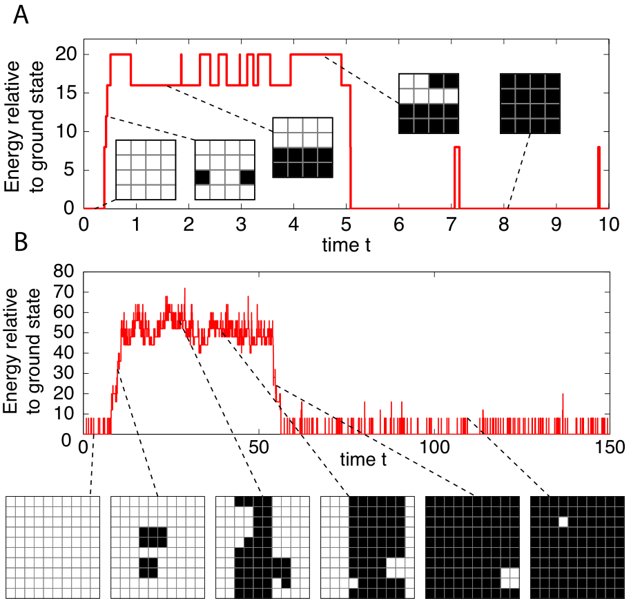
Our method allows us to inspect actual transition paths in detail. In Fig. 11 we show two examples of snapshots transition paths, at small () and large () sizes. The films of the full transition paths are available as supplementary documents. These examples show how the system first creates a stripe of up spins in a background of down spins. This stripe then progressively invades the lattice.
IV.1.3 Computer time
To conclude this section we want to give an order of magnitude of the computer time that was needed to obtain the above results. We want to stress, however, that our code was not particularly optimized for the model we investigated, but it just corresponds to a plain implementation of the algorithm described above. We believe that its performances might be improved by some smart optimizations, which are beyond the scope of this work.
The simulations were conducted on standard workstations, equipped with Intel Core i7 CPUs running at 2.80 GHz. For the smallest systems, e.g. at and , the calculation requires of the order of one day of CPU time to obtain very accurate results. For the largest system we simulated ( and , corresponding to the rightmost black point in lower panel of Fig. 9), a single point of thermodynamic integration required a computational time of the order of one month. The thermodynamic integration required running 12 independent values of temperature, therefore obtaining for and required a total of almost 1 year of CPU time (which of course was possible in a much shorter time by using a small cluster of 48 cores). The computational time for a given system scales as , which is the “system size”. Overall, we believe that this is a good performance, because the value of the rate at is extremely small (), so we are looking to really rare events.
Of course, as for any Monte Carlo simulation, the computational time depends crucially on the desired statistics. Given the complexity of the procedure, we were unable to estimate error bars in a reliable way, however we roughly estimate them to be of the order of symbol sizes in Fig. 9, which we believe to be sufficient for the present purposes.
A final remark is that the computation of turns out to be much easier than that of on the same state point. This is related to the following observation. Typical configurations of the paths are given in Fig. 11, and they are characterized by periods of inactivity (in which all spins are up or down) separated by the barrier crossing period, where the energy is above the ground state. The position of the latter period fluctuates uniformly and slowly during the path Monte Carlo simulation. Remarkably, the value of is independent of the time location of the barrier crossing, therefore one does not need to accumulate much statistics on the slow fluctuations of the latter to have a reliable result on this quantity. On the contrary, the calculation of clearly requires a perfect sampling of the fluctuations of the barrier crossing point. Achieving this seems much more difficult and for this reason this quantity is typically much more noisy. For this reason we found that the results of thermodynamic integration (black dots in figure 9) were typically much more reliable that the ones obtained through (red and blue lines in Fig. 9).
IV.2 Interpretation
IV.2.1 Transition state and surface tension
In the limit of large system sizes, simple arguments allow us to write the scaling of the transition rate in terms of the surface tension, . If we imagine starting from a homogenous system in which all spins are aligned, the transition time depends on the probability of the initial nucleation event of the first stripe of spins of opposite sign. The escape time is then simply proportional to the exponential of surface tension of that stripe, times its surface ( is the length or linear dimension of the system, and the stripe has two interfaces) [18]:
| (53) |
The surface tension in a 2D Ising model has been calculated exactly in the thermodynamic limit by Onsager, and its value is [15, 16, 17, 18]. However, a simple model [27] allows to obtain an approximated expression for the surface tension also at finite size. In this simplified model, illustrated in Fig. 12, an interface between a plus and minus region is described by a single-valued function , neglecting overhangs. At the left and right boundary the interface is supposed to be in . The energy associated with the interface is
| (54) |
and its partition function is therefore
| (55) |
which is easily computed by Fourier transform:
| (56) |
The corresponding surface tension is .
The result is that at small and large enough , the partition function is dominated by the configuration and tends to be rectilinear, thereby losing the benefit of the entropic contribution to the surface tension. Such a rectilinear boundary leads to . On the contrary, for large the integral in Eq. (56) can be evaluated by a saddle-point and gives the exact result of Onsager, including the entropic contribution. The crossover between these two regimes happens at a length scale that is extremely small close to , and grows with decreasing temperature, diverging at . From Eq. (56), we find that at the crossover indeed happens around .
These results are consistent with the data we reported in Figure 1. Indeed, the slope at small is consistent with a higher surface tension (in units of , and for ). As increases, the slope asymptotically approaches the correct value given by the Onsager formula.
IV.2.2 Transient time
We find that the transient time grows linearly with . Let us try to interpret this result. The transient time may be interpreted as the minimum time for the transition to occur. This time is at least as long as the time the system takes to relax to state after starting at the top the barrier between and . In our case, the top of the barrier corresponds to configurations where a stripe of up spins has nucleated across the system’s length in a background of down spins. Let us reason at low enough temperature, where the stripe is almost perfectly rectilinear and where defects are extremely rare. We expect our reasoning to hold for arbitrary temperatures. In order to invade the lattice entirely, the stripe needs to thicken by adding new layers of up spins on either of its sides. Likewise, the stripe may thin out through the removal of spin layers. The thickness of the stripe therefore undergoes an unbiased random walk (Fig. 13A). If the rate of adding or removing layers to the stripe is , then the expected time for the stripe to invade the system is the time it takes for the random walk to reach the system’s length, . This time scales as . The rate itself can be estimated in a similar manner (Fig. 13B). A new layer can be added when an up spin appears sticking out from one of the two stripe’s boundaries, incurring a energy cost. Once such a defect has been created, adding or removing up spins on the same layer contiguously to the defect—to make it bigger or smaller—has no energy cost. The length of the defect is therefore governed by a random walk, which ends when the defect disappears or creates a new layer of up spins by reaching the system’s length . Layer removal occurs is the exact same way, and therefore . In summary, we expect the transient time to scale with as , in agreement with our results. It seems that the prefactor of this scaling depends on the surface tension, since we observe that it changes around the same length scale as in Fig. 1.
V Conclusions
We have presented a method for efficiently sampling transition trajectories of discrete systems. The method is general and applicable to systems in and out of equilibrium. The method scales well with system size and we are able to effectively sample trajectories in systems for which asymptotic scaling holds. We emphasize two main advantages of the method presented in this paper. Firstly, the method does not require detailed balance to hold and is therefore applicable to all nonequilibrium systems. Secondly, the method scales reasonably with the number of variables in the system, allowing one to calculate the escape rates for otherwise prohibitively large problems. Combined with a thermodynamic integration procedure, it gives detailed information on the typical transition paths, the full time-dependent transition probability , the transition rate , and the transient time , which is related to the minimal barrier crossing time. We tested our method on the equilibrium example of a 2D Ising model with periodic boundary conditions, where we achieved excellent agreement between the results of the path sampling method to exact matrix diagonalization and predictions for asymptotic scaling.
Our method is based on the classical path sampling method of Dellago et al. for continuous variables [5], which is based on the idea of avoiding performing a detailed Monte Carlo simulation on the variables of the system, but instead to propose a Monte Carlo algorithm on the paths themselves, and on the use of thermodynamic integration to compute the transition rate.
Our new implementation of the path sampling takes advantage of the discrete and many-body nature of the system. It allows us to consider the trajectories for each variable separately and modify them while keeping the rest of the system fixed. As a result we can draw a whole new trajectory for the chosen spin, instead of just modifying it locally. We expect this procedure to be more efficient in sampling the space of paths. We also solved a technical issue that is specific to many-body systems, namely the fact that the thermodynamic integration on the final state proposed in [5] fails because a first order phase transition is met on the integration path. We performed instead a thermodynamic integration in temperature; thermodynamic quantities are smooth on this path, allowing for an accurate computation. We expect this to be a generic phenomenon for many-body systems.
A direct comparison with the performances of other methods is not straightforward. Some of these methods have been applied on the 2D Ising model [25, 26] but the nucleation problem studied there was different (nucleation in presence of an external magnetic field). Also, all these methods are complex enough that the actual performances depend a lot on the implementation and the details of the problem under investigation. We believe that the important point is that the present method scales linearly with the “size” of the path system, (note however that the time typically grows polynomially with system size, e.g. in this case, meaning that the overall computational time is expected to scale polynomially in with some exponent larger than 1). Thanks to this, we believe that the method gives an interesting way to study discrete many-body problems and obtain complementary information to other techniques.
The method can be straightforwardly applied to study the dynamics of disordered spin systems, chemical reactions and gene regulatory systems. In these last two classes of problems, one needs to consider the numbers of molecules that take part in the reactions—a number that is in principle infinite, but usually bounded in practice. The method presented here is still applicable to such problems. Although the purpose of the present paper is to introduce the method in a clear way and convincingly show agreement with well known results on an equilibrium example, future work should focus on non-equilibrium applications.
A very interesting property of this method is that it allows us to examine typical sample trajectories and get a detailed picture of the transition, with e.g. the detailed shape and dynamics of the critical nucleus in the 2D Ising model. In particular, we get complete access to the time-dependent cumulative transition probability , which tells us the probability that the system undergoes a transition even for very short times when the process is not yet Poissonian—i.e. for times shorter than the typical relaxation time. In the 2D Ising model, we estimated this transient time and discussed its scaling with the system’s size. The estimation of at short times might also be important for some biological applications where one deals with large microbial populations. In such problems, the rarity of transition events in gene-regulatory or biochemical networks is compensated by very large size of populations, which makes that nominally rare events occur quite often at the population level. In this context, may for example be interpreted as the fraction of individuals that make a potentially life-saving transition within some finite time after the introduction of a stress. Our method provides the tools to estimate such tiny fractions in models of biochemical networks [29, 30].
Acknowledgements.
We would like to warmly thank Patrick Charbonneau, Zoran Ristivojevic, and Guilhem Semerjian for several crucial discussions. We acknowledge the support of the Projet Incitatif de Recherche 2011 grant from the École normale supérieure.Appendix A Detailed calculations for the mean field model
A.1 Master equation
Because the Hamiltonian depends only on , it follows that at any time , depends only on too (provided this is true at ). Therefore we can write:
| (57) |
Injecting the above equation into Eqn. (6), and using the relation
| (58) |
it is easy to show that
| (59) |
with
| (60) |
which has the form of a one-dimensional birth-death process [23, Section 7.1].
A.2 Mean first-passage time
We then use the results of [23, Section 7.4] for discrete, one-dimensional birth-death processes in order to compute the mean first passage time in of a system that starts in at time (hence we are taking the negative state as the initial state, and the positive state as the final state). Obviously the system is confined by a reflecting barrier in . Using this and [23, Eq. (7.4.12)], we get (in the following sums, capital letter denote magnetizations and therefore increase in steps of 2 units)
| (61) |
with
| (62) |
The latter expression can be computed numerically for finite , in a time growing only polynomially in .
A.3 Large limit
We want to study the large asymptotic behaviour of Eq. (61). We note that using Eq. (8) we have where is the derivative of the free energy in Eq. (15). Therefore,
| (63) |
with
| (64) |
To estimate the correction , we need to separate the free energy in Eq. (15) in two terms:
| (65) |
where the second term is singular at . Likewise, we separate into a regular and a singular term. For the first term, we can use that , and therefore
| (66) |
For the singular term, we can use the explicit form of the second term in (65) to write
| (67) |
where the last line can be obtained by recognizing that the sum can be written as a convergent part plus a divergent sum which is the harmonic number, and then using the asymptotic expression of the latter. We get the final result
| (68) |
Next we evaluate the sum
| (69) |
where the second line is obtained via the saddle point method. The saddle point is at , and we assumed that which is the case that will be relevant in the following. We also used the symmetry .
Finally, recalling Eq. (61):
| (70) |
Assuming that and , we can again evaluate the integral by a saddle point, the saddle point being in in this case:
| (71) |
Simplifying this expression leads to the final result
| (72) |
as reported in Eq. (16).
We notice that the above result is independent of provided they scale proportionally to . Alternatively, one can consider a scaling regime where and , in which case
| (73) |
with . This scaling regime is the one where the mean first passage time depends on the initial and final points.
A.4 Calculation of
For the mean-field model, the function can be defined as follows:
| (74) |
where the operator is defined in Eq. (59), is an initial probability distribution which is assumed to be centered on state , and is the indicator function of state , i.e. it is one when the system is in state and zero otherwise.
This quantity can be easily computed. Recalling that the invariant distribution is
| (75) |
we can define a symmetric matrix
| (76) |
which can be easily diagonalized helding eigenvalues and (negative) eigenvectors , and
| (77) |
To produce the plots of Fig. 3, we chose as a definition of the states and the following functions:
| (78) |
with , and . However, the shape of is largely independent of the details of these definitions.
References
- [1] P. Haenggi, P. Talkner and M. Borkovec, Reaction-rate theory: fifty years after Kramers, Rev. Mod. Phys. 62, 251 (1990).
- [2] R.J. Allen, C.Valeriani and P. Rein ten Wolde, Forward flux sampling for rare event simulations, Journal of Physics: Condensed Matter 21, 463102 (2009).
- [3] C. H. Bennett, Algorithms for Chemical Computations (ACS Symposium, Series No. 46) ed R Christofferson (Washington, DC: American Chemical Society) (1977)
- [4] J. Hu, A. Ma and A.R. Dinner, Bias annealing: a method for obtaining transition paths de novo, J. Chem. Phys. 125, 114101 (2006).
- [5] C. Dellago, P. G. Bolhuis, F. S. Csajka, and D. Chandler, Transition Path Sampling and the Calculation of Rate Constants, Journal of Chemical Physics 108, 1964 (1998).
- [6] C. Dellago, P. G. Bolhuis and P. L. Geissler, Adv. Chem. Phys. 123, 1 (2002).
- [7] R. J. Allen , P. B. Warren and P. Rein ten Wolde, Sampling rare switching events in biochemical networks, Physical Review Letters 94, 018104 (2005).
- [8] W. E, W. Ren and E. Vanden-Eijnden, String method for the study of rare events, Phys. Rev. B. 66, 052301 (2002).
- [9] W. E, W. Ren and E. Vanden-Eijnden, Finite temperature string method for the study of rare events, J. Phys.Chem. B 109, 6688 (2005).
- [10] J. Tailleur, S. Tanase-Nicola, J. Kurchan, Kramers equation and supersymmetry, J. Stat. Phys. 122, 557 (2006).
- [11] C. Giardina, J. Kurchan, V. Lecomte and J. Tailleur, Simulating Rare Events in Dynamical Processes, J. Stat. Phys. 145, 787 (2011).
- [12] M. Picciani, M. Athènes, J. Kurchan, J. Tailleur, Simulating structural transitions by direct transition current sampling: the example of LJ38, J. Chem. Phys. 135, 034108 (2011).
- [13] F.Krzakala, A.Rosso, G.Semerjian and F.Zamponi, Path integral representation for quantum spin models and its application to the quantum cavity method and to Monte Carlo simulations, Phys. Rev. B 78, 134428 (2008).
- [14] R. B. Griffiths, C. Y. Weng and J. S. Langer, Phys.Rev. 149, 301 (1966).
- [15] L. Onsager, Phys. Rev. 65, 117 (1944).
- [16] G. Gallavotti, Instabilities and Phase Transitions in the Ising Model. A Review, Rivista del Nuovo Cimento 2, 133 (1972); D. Abraham, G. Gallavotti and A. Martin-Lof, Lettere al nuovo cimento 2, 143 (1971); G. Gallavotti, A. Martin-Lof, and S. Miracles-Solé, Lecture Notes in Physics 20, 162 (1971).
- [17] K. Binder, Monte Carlo calculation of the surface tension for two- and three-dimensional lattice-gas models, Phys. Rev. A 25, 1699 (1982)
- [18] F. Martinelli, On the two dimensional dynamical Ising model in the phase coexistence region, J. Stat. Phys. 76, 1179 (1994); E. Marcelli and F. Martinelli, Some new results on the kinetic Ising model in the phase coexistence region, J. Stat.Phys. 84, 655 (1996); F. Cesi, G. Guadagni, F. Martinelli and R.H. Schonmann: On the two-dimensional stochastic Ising model in the phase coexistence region close to the critical point, J. Stat. Phys. 85, 55 (1996); F.Martinelli, Lectures on Glauber dynamics for discrete spin models, in Lectures on Probability Theory and Statistics (Saint-Flour, 1997), Lecture Notes in Mathematics, Vol. 1717, Springer, Berlin, 1999, pp. 93–191.
- [19] J. Wang and P. G. Wolynes, Survival Paths for Reaction Dynamics in Fluctuating Environments, Chem. Phys. 180, 141 (1994).
- [20] S. Kauffman, The Origins of Order: Self-Organization and Selection in Evolution, Oxford University Press, USA; 1 edition (June 10, 1993)
- [21] W. Krauth, Statistical mechanics: algorithms and computations, Oxford University Press (2006).
- [22] S. Redner, A Guide to First-Passage Processes, Cambridge University Press (August 6, 2001)
- [23] C. W. Gardiner, Handbook of Stochastic Methods: For Physics, Chemistry and Natural Sciences, Springer Verlag, 2nd edition (January 1985).
- [24] M. Suzuki, Prog. Th. Phys. 56, 1454 (1976).
- [25] C. Valeriani, R.J. Allen, M.J.Morelli, D.Frenkel, and P.Rein ten Wolde, Computing stationary distributions in equilibrium and nonequilibrium systems with forward flux sampling, J.Chem.Phys. 127, 114109 (2007); R J. Allen, C. Valeriani, S.Tanase-Nicola, P. Rein ten Wolde and D. Frenkel, Homogeneous nucleation under shear in a two-dimensional Ising model:cluster growth, coalescence, and breakup, J. Chem. Phys. 129, 134704 (2008).
- [26] M. Venturoli, E. Vanden-Eijnden, G. Ciccotti, Kinetics of phase transitions in two dimensional Ising models studied with the string method, J. Math. Chem. 45, 188 (2009).
- [27] E. Muller-Hartmann and J. Zittarz, Z. Phys. B 27, 261 (1977).
- [28] Y. Bakhtin, preprint arXiv:1005.4964.
- [29] G.M. Süel, J. Garcia-Ojalvo, L.M. Liberman and M.B Elowitz, An excitable gene regulatory circuit induces transient cellular differentiation, Nature 440, 545 (2006).
- [30] M. Acar, A. Becskei, and A. van Oudenaarden, Enhancement of cellular memory by reducing stochastic transitions, Nature 435, 228 (2005).