New Geometrical Spectra of Linear Codes with Applications to Performance Analysis

The sequence $\{A_{i},0\leq i\leq n\}$ is also called weight spectrum of the code, which exhibits how many codewords that are $i$ positions far away from the reference codeword $\underline{c}^{(0)}$. By linearity, we know that the weight spectrum is irrelevant to the reference codeword. Clearly, we have

For a binary code with the all-one codeword, we further have $A_{i}=A_{n-i}$ for $0\leq i\leq n$.

Generally, the TrEF depends on the choice of the reference codeword $\underline{c}^{(1)}$. When the context is clear, we may drop the reference codeword from the notation. The sequence $\{B_{i,j},0\leq i,j\leq n\}$ is also called the triangle spectrum of the code. Clearly, we have

For binary codes with the all-one codeword, we have the following proposition.

Generally, the TeEF depends on the choice of the reference codewords $\underline{c}^{(1)}$ and $\underline{c}^{(2)}$. When the context is clear, we may drop the reference codewords from the notation. The sequence $\{C_{i,j,h},0\leq i,j,h\leq n\}$ is also called the tetrahedron spectrum of the code. Clearly, we have

We take the Hamming code $\mathcal{C}_{2}[7,4]$ as an example to illustrate the introduced enumerating functions.

The WEF is

Since the TrEF depends on the choice of the reference codeword $\underline{c}^{(1)}$, we distinguish following three cases.

1. Case 1: If $W_{H}(\underline{c}^{(1)})=7$,

   $$B(X,Y)=Y^{7}+7X^{3}Y^{4}+7X^{4}Y^{3}+X^{7}.$$

2. Case 2: If $W_{H}(\underline{c}^{(1)})=4$,

   $$B(X,Y)=Y^{4}+X^{4}+6X^{3}Y^{3}+X^{3}Y^{7}+6X^{4}Y^{4}+X^{7}Y^{3}.$$

3. Case 3: If $W_{H}(\underline{c}^{(1)})=3$,

   $$B(X,Y)=Y^{3}+X^{3}+6X^{3}Y^{4}+6X^{4}Y^{3}+X^{4}Y^{7}+X^{7}Y^{4}.$$

Similarly, the TeEF also depends on the choices of the reference codewords $\underline{c}^{(1)}$ and $\underline{c}^{(2)}$. We have

1. Case 1: If $W_{H}(\underline{c}^{(1)})=3$ and $W_{H}(\underline{c}^{(2)})=3$,

   $$\begin{array}[]{l}C(X,Y,Z)=Y^{3}Z^{3}+X^{3}Y^{4}+X^{3}Z^{4}+\\ 5X^{3}Y^{4}Z^{4}+5X^{4}Y^{3}Z^{3}+X^{4}Y^{3}Z^{7}+X^{4}Y^{7}Z^{3}+X^{7}Y^{4}Z^{4}.\end{array}$$

2. Case 2: If $W_{H}(\underline{c}^{(1)})=3$, $W_{H}(\underline{c}^{(2)})=4$, and $W_{H}(\underline{c}^{(2)}-\underline{c}^{(1)})=3$,

   $$\begin{array}[]{l}C(X,Y,Z)=Y^{3}Z^{4}+X^{3}Z^{3}+X^{4}Y^{3}+\\ 5X^{3}Y^{4}Z^{3}+X^{3}Y^{4}Z^{7}+5X^{4}Y^{3}Z^{4}+X^{4}Y^{7}Z^{4}+X^{7}Y^{4}Z^{3}.\end{array}$$

3. Case 2’: If $W_{H}(\underline{c}^{(1)})=3$, $W_{H}(\underline{c}^{(2)})=4$, and $W_{H}(\underline{c}^{(2)}-\underline{c}^{(1)})=7$,

   $$\begin{array}[]{l}C(X,Y,Z)=Y^{3}Z^{4}+X^{3}Z^{7}+X^{4}Y^{7}+\\ 6X^{3}Y^{4}Z^{3}+6X^{4}Y^{3}Z^{4}+X^{7}Y^{4}Z^{3}.\end{array}$$

4. Case 3: If $W_{H}(\underline{c}^{(1)})=3$ and $W_{H}(\underline{c}^{(2)})=7$,

   $$\begin{array}[]{l}C(X,Y,Z)=Y^{3}Z^{7}+X^{3}Z^{4}+X^{7}Y^{4}+\\ 6X^{3}Y^{4}Z^{4}+6X^{4}Y^{3}Z^{3}+X^{4}Y^{7}Z^{3}.\end{array}$$

5. Case 4: If $W_{H}(\underline{c}^{(1)})=4$ and $W_{H}(\underline{c}^{(2)})=4$,

   $$\begin{array}[]{l}C(X,Y,Z)=Y^{4}Z^{4}+X^{4}Z^{4}+X^{4}Y^{4}+\\ 5X^{3}Y^{3}Z^{3}+X^{3}Y^{3}Z^{7}+X^{3}Y^{7}Z^{3}+5X^{4}Y^{4}Z^{4}+X^{7}Y^{3}Z^{3}.\end{array}$$

6. Case 5: If $W_{H}(\underline{c}^{(1)})=4$ and $W_{H}(\underline{c}^{(2)})=7$,

   $$\begin{array}[]{l}C(X,Y,Z)=Y^{4}Z^{7}+X^{4}Z^{3}+X^{7}Y^{3}+\\ 6X^{3}Y^{3}Z^{4}+X^{3}Y^{7}Z^{4}+6X^{4}Y^{4}Z^{3}.\end{array}$$

It is well-known that any linear block code can be represented by a trellis [12] [13]. Generally, a trellis that represents $\mathcal{C}_{q}[n,k]$ can have $N$ stages. The trellis section at stage $t$ ($0\leq t\leq N-1$), denoted by $\mathcal{B}_{t}$, is a subset of $\mathcal{S}_{t}\times\mathbb{F}_{q}^{n_{t}}\times\mathcal{S}_{t+1}$, where $\mathcal{S}_{t}$ is the state space at time $t$. A branch $b\in\mathcal{B}_{t}$ is denoted by $b\stackrel{{\scriptstyle\Delta}}{{=}}(\sigma^{-}(b),\ell(b),\sigma^{+}(b))$, starting from a state $\sigma^{-}(b)\in\mathcal{S}_{t}$, taking a label $\ell(b)\in\mathbb{F}_{q}^{n_{t}}$, and ending into a state $\sigma^{+}(b)\in\mathcal{S}_{t+1}$. A path through a trellis is a sequence of branches ${\underline{b}}=(b_{0},b_{1},\cdots,b_{N-1})$ satisfying that $b_{t}\in\mathcal{B}_{t}$ and $\sigma^{-}(b_{t+1})=\sigma^{+}(b_{t})$. A codeword is then represented by a path in the sense that $\underline{c}=(\ell(b_{0}),\ell(b_{1}),\cdots,\ell(b_{N-1}))$. Naturally, $\sum_{0\leq t\leq N-1}n_{t}=n$ and the number of paths is $q^{k}$. Without loss of generality, we set $\mathcal{S}_{0}=\mathcal{S}_{N}=\{0\}$.

Let $\mathbb{F}_{2}=\{0,1\}$ and $\mathcal{A}_{2}=\{-1,+1\}$ be the binary field and the bipolar signal set, respectively. Suppose that a codeword $\underline{c}=(c_{0},c_{1},\cdots,c_{n-1})\in\mathcal{C}_{2}[n,k]$ is modulated by binary phase shift keying (BPSK), resulting in a bipolar signal vector $\underline{s}\in\mathcal{A}_{2}^{n}$ with $s_{t}=1-2c_{t}$ for $0\leq t\leq n-1$. We will not distinguish between a binary codeword $\underline{c}$ and its bipolar image in the following, except when we need to emphasize the difference between the Hamming space $\mathbb{F}_{2}^{n}$ and the Euclidean space $\mathbb{R}^{n}\supset\mathcal{A}_{2}^{n}$. The Euclidean distance between two codewords $\underline{s}^{(1)}$ and $\underline{s}^{(2)}$ is related to their Hamming distance by $\|\underline{s}^{(2)}-\underline{s}^{(1)}\|=2\sqrt{W_{H}(\underline{c}^{(2)}-\underline{c}^{(1)})}$. All codewords are distributed on the surface of an $n$-dimensional sphere centered at the origin with radius $\sqrt{n}$. This property is referred to as the sphericity of the bipolar code.

Assume that a codeword $\underline{s}$ is transmitted over an AWGN channel, resulting in a received vector $\underline{y}={\underline{s}}+{\underline{z}}$, where $\underline{z}$ is a sample from a white Gaussian noise process with zero mean and double-sided power spectral density $\sigma^{2}$. The ML decoding is equivalent to finding a bipolar codeword $\underline{s}$ that is the closest to $\underline{y}$. Since the decoding metric is the Euclidean distance, the geometrical structure of the code in $\mathbb{R}^{n}$ is supposed to be critical to analyze the ML decoding performance. However, to the best knowledge of ours, with the exception of the distance spectrum and the sphericity of the code, other figures of merits of the code were rarely employed to upper bound the ML decoding error probability. To reveal more information about the geometrical structure of the code, we have the following two propositions, where Proposition 3 was originally mentioned in [14] without proofs.

Assume that ${\underline{s}}^{(0)}$ is transmitted. For a codeword $\underline{s}$, let

which is the event that $\underline{s}$ is nearer than $\underline{s}^{(0)}$ to $\underline{y}$. We use $\{\underline{s}^{(0)}\nrightarrow\underline{s}\}$ to denote the complementary event.

To derive the upper bounds on the decoding error probability ${\rm Pr}\{E\}$, we take two arbitrary but fixed codewords ${\underline{s}^{(1)}}$ and ${\underline{s}^{(2)}}$ as reference codewords. Let $d_{1}=W_{H}(\underline{c}^{(1)})$, $d_{2}=W_{H}(\underline{c}^{(2)})$ and $d_{1,2}=W_{H}(\underline{c}^{(1)}-\underline{c}^{(2)})$. For a codeword $\underline{c}$, let $i=W_{H}(\underline{c}-\underline{c}^{(0)})$, $j=W_{H}(\underline{c}-\underline{c}^{(1)})$ and $h=W_{H}(\underline{c}-\underline{c}^{(2)})$. It is well-known that the pair-wise error probability (PEP) $p_{2}(i)\stackrel{{\scriptstyle\Delta}}{{=}}{\rm Pr}\{\underline{s}^{(0)}\rightarrow\underline{s}\}$ is given by $Q(\sqrt{i}/\sigma)$ and depends solely on the Hamming weight. Going a step further, we can verify that the triplet-wise error probability (TrEP), defined by

depends solely on the triangle formed by the three codewords. Similarly, the quadruple-wise error probability (QuEP), defined by

depends solely on the tetrahedron (or rectangle) formed by the four codewords. For these reasons, we have dropped the codeword $\underline{s}$ from the notation and simply denoted these probabilities by $p_{2}(i)$, $p_{3}(i,j)$ and $p_{4}(i,j,h)$ as shown above.

To compute the introduced error probabilities conveniently, we may use a new coordinate system by choosing $\underline{s}^{(0)}$ as the origin $O$ and taking $\overrightarrow{\underline{s}^{(0)}\underline{s}^{(1)}}$ as an axis, denoted by $\xi_{1}$-coordinate. We further choose $\xi_{2}$-coordinate such that $\underline{s}^{(2)}$ falls into the first quadrant of the plane $\xi_{1}O\xi_{2}$. Similarly, we choose $\xi_{3}$-coordinate such that the fourth codeword $\underline{s}$ falls in the first octant, as shown in Fig. 2. Note that such an arrangement does not lose any generality. Let $Z_{\xi_{1}}$, $Z_{\xi_{2}}$, and $Z_{\xi_{3}}$ be the three components obtained by projecting the noise $\underline{Z}$ onto the three axes, respectively. Specifically, $Z_{\xi_{1}}$ is the inner product $\langle{\underline{Z}},\frac{\underline{s}^{(1)}-\underline{s}^{(0)}}{\|\underline{s}^{(1)}-\underline{s}^{(0)}\|}\rangle$. These three component are independent and identically distributed as a Gaussian random variable with a probability density function $f(x)=\frac{1}{\sqrt{2\pi}\sigma}\exp\{-\frac{x^{2}}{2\sigma^{2}}\}$. We have the following lemmas.

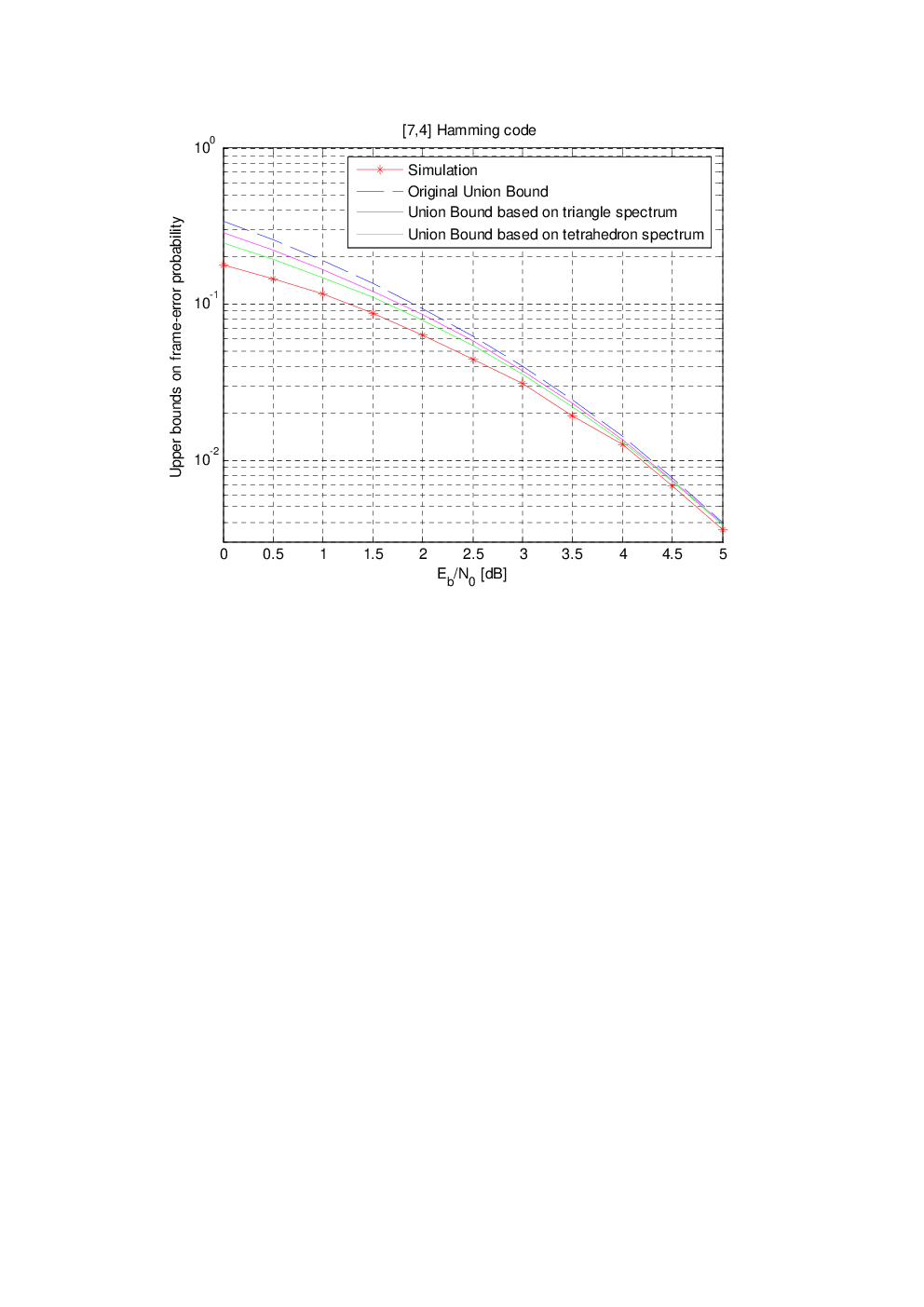
From the proofs of Theorems 1 and 2, we know that the proposed bounds compute the higher-order Bonferroni-type inequalities. Hence the proposed bounds are tighter than the conventional union bound. To verify this numerically, we give an example. Fig. 3 shows the comparisons between the original union bound and the bounds given in Theorems 1 and 2 on the frame-error probability of the Hamming code $\mathcal{C}_{2}[7,4]$. Also shown are the simulation results. The TrEF and TeEF we choose are $B(X,Y)=Y^{3}+X^{3}+6X^{3}Y^{4}+6X^{4}Y^{3}+X^{4}Y^{7}+X^{7}Y^{4}$ and $C(X,Y,Z)=Y^{3}Z^{3}+X^{3}Y^{4}+X^{3}Z^{4}+5X^{3}Y^{4}Z^{4}+5X^{4}Y^{3}Z^{3}+X^{4}Y^{3}Z^{7}+X^{4}Y^{7}Z^{3}+X^{7}Y^{4}Z^{4}$, respectively. We can see that the bounds using higher-order Bonferroni-type inequalities are tighter, as expected.

References

- [1] F. J. MacWilliams and N. J. A. Sloane, The theory of error correcting codes. New York: North Holland Publishing Co., 1977.
- [2] I. Sason and S. Shamai, “Performance analysis of linear codes under maximum-likelihood decoding: A tutorial,” in Foundations and Trends in Communications and Information Theory. Delft, The Netherlands: NOW, July 2006, vol. 3, no. 1-2, pp. 1–225.
- [3] E. R. Berlekamp, “The technology of error correction codes,” Proceedings of the IEEE, vol. 68, pp. 564–593, May 1980.
- [4] T. Kasami, T. Fujiwara, T. Takata, K. Tomita, and S. Lin, “Evaluation of the block error probability of block modulation codes by the maximum-likelihood decoding for an AWGN channel,” in Proc. of the 15th Symposium on Information Theory and Its Applications, Minakami, Japan, September 1992.
- [5] H. Herzberg and G. Poltyrev, “Techniques of bounding the probability of decoding error for block coded modulation structures,” IEEE Transactions on Information Theory, vol. 40, pp. 903–911, May 1994.
- [6] G. Poltyrev, “Bounds on the decoding error probability of binary linear codes via their spectra,” IEEE Transactions on Information Theory, vol. 40, pp. 1284–1292, July 1994.
- [7] J. Zangl and R. Herzog, “Improved tangential sphere bound on the bit error probability of concatenated codes,” IEEE Journal on Selected Areas in Communications, vol. 19, pp. 825–830, May 2001.
- [8] D. Divsalar and E. Biglieri, “Upper bounds to error probabilities of coded systems beyond the cutoff rate,” IEEE Trans. Commun., vol. 51, no. 12, pp. 2011–2018, December 2003.
- [9] S. Yousefi and A. K. Khandani, “A new upper bound on the ML decoding error probability of linear binary block codes in AWGN interference,” IEEE Transactions on Information Theory, vol. 50, pp. 3026–3036, Novomber 2004.
- [10] A. Mehrabian and S. Yousefi, “Improved tangential sphere bound on the ML decoding error probability of linear binary block codes in AWGN and block fading channels,” IEE Proc. Commun., vol. 153, pp. 885–893, December 2006.
- [11] X. Ma, J. Liu, and B. Bai, “New techniques for upper-bounding the MLD performance of binary linear codes,” in Proc. 2011 IEEE Int. Symp. Inform. Theory, Saint-Petersburg, Russian Federation, August 2011.
- [12] R. J. McEliece, “On the BCJR trellis for linear block codes,” IEEE Transactions on Information Theory, vol. 42, pp. 1072–1092, July 1996.
- [13] A. Vardy, “Trellis structure of codes,” in Handbook of Coding Theory, V. S. Pless and W. C. Huffman, Eds. Amsterdam, The Netherlands: Elsevier, 1998, vol. 2.
- [14] E. Agrell, “On the Voronoi neighbor ratio for binary linear block codes,” IEEE Transactions on Information Theory, vol. 44, pp. 3064–3072, Novomber 1998.