Excitation of collective modes in a quantum flute

Kristinn Torfason Affiliation: School of Science and Engineering, Reykjavik University, Menntavegur 1, IS-101 Reykjavik, Iceland Affiliation: Science Institute, University of Iceland, Dunhaga 3, IS-107 Reykjavik, Iceland Andrei Manolescu Affiliation: School of Science and Engineering, Reykjavik University, Menntavegur 1, IS-101 Reykjavik, Iceland Valeriu Molodoveanu Affiliation: National Institute of Materials Physics, P. O. Box MG-7, Bucharest-Magurele, Romania Vidar Gudmundsson Affiliation: Science Institute, University of Iceland, Dunhaga 3, IS-107 Reykjavik, Iceland

August 24, 2026

Abstract

We use a generalized master equation (GME) formalism to describe the non-equilibrium time-dependent transport of Coulomb interacting electrons through a short quantum wire connected to semi-infinite biased leads. The contact strength between the leads and the wire is modulated by out-of-phase time-dependent potentials which simulate a turnstile device. We explore this setup by keeping the contact with one lead at a fixed location at one end of the wire whereas the contact with the other lead is placed on various sites along the length of the wire. We study the propagation of sinusoidal and rectangular pulses. We find that the current profiles in both leads depend not only on the shape of the pulses, but also on the position of the second contact. The current reflects standing waves created by the contact potentials, like in a wind musical instrument (for example a flute), but occurring on the background of the equilibrium charge distribution. The number of electrons in our quantum ”flute” device varies between two and three. We find that for rectangular pulses the currents in the leads may flow against the bias for short time intervals, due to the higher harmonics of the charge response. The GME is solved numerically in small time steps without resorting to the traditional Markov and rotating wave approximations. The Coulomb interaction between the electrons in the sample is included via the exact diagonalization method. The system (leads plus sample wire) is described by a lattice model.

pacs

72.15.Nj, 73.23.Hk, 78.47.da, 85.35.Be

I Introduction

The control of transient transport properties of open nanodevices subjected to time-dependent signals is nowadays considered as the main tool for charge and spin manipulation. Pump-and-probe techniques allow the indirect measurement of tunneling rates and relaxation times of quantum dots in the Coulomb blockade [1]. Quantum point contacts and quantum dots submitted to pulses applied only to the input lead generate specific output currents [2, 3, 4]. Single electrons pumping through a double quantum dot defined in an InAs nanowire by periodic modulation of the wire potential has been observed [5], as well as non-adiabatic monoparametric pumping in AlGaAs/GaAs gated nanowires [6].

Modeling such short-time processes is a serious task because even if the charge dynamics is imposed by the time-dependent driving fields, the geometry of the sample itself and the Coulomb interaction play also an important role. A well-established approach to time-dependent transport relies on the non-equilibrium Greens’ function (NEGF) formalism, the Coulomb effects being treated either via density-functional methods [7] or within many-body perturbation theory [8]. Alternatively, equation of motion methods were used for studying pumping in finite and infinite- $U$ Anderson single-level models [9]. The numerical implementation of these formal methods in the interacting case requires extensive and costly computational work if the sample accommodates more than few electrons; as a consequence, accurate simulations for systems having a more complex geometry and/or complex spectral structure are not easily obtained.

Recently we reported transport calculations for a two-dimensional parabolic quantum wire in the turnstile setup [10], neglecting the Coulomb interaction between electrons in the wire. The latter is connected to semi-infinite leads seen as particle reservoirs. Let us remind here that the turnstile setup was experimentally realized by Kouwenhoven et al. [11]. It essentially involves a time-dependent modulation (pumping) of the tunneling barriers between the finite sample and drain and source leads, respectively. During the first half of the pumping cycle the system opens only to the source lead whereas during the second half of the cycle the drain contact opens. At certain values of the relevant parameters an integer number of electrons is transferred across the sample in a complete cycle. More complex turnstile pumps have been studied by numerical simulations, like one-dimensional arrays of junctions [12] or two-dimensional multidot systems [13].

In this work we perform a similar study for an interacting one-dimensional quantum wire coupled to an input (source) lead at one end, while the output (drain) lead can be plugged at any point along its length. Both contacts are modulated by periodic pulses (sinusoidal or square shaped). Our study is motivated by the possibility to control the transient currents through the variation of the drain contact. We shall see in fact that the flexibility of the drain contact allows us to capture different responses of the sample to local time-dependent perturbations which can lead to transient currents with specific shapes. In some sense, our system works like a ‘quantum flute’, this fact being revealed when analyzing the distribution of charge within the wire. In particular, we calculate and discuss the deviation of the charge density from the mean value for each site of the quantum wire and observe the onset of standing waves.

The effect of the electron-electron interaction is included in the sample via the exact diagonalization method while the time-dependent transport is performed within the generalized master equation (GME) formalism as it is described in Ref. 14. The implemented GME formalism can be used to describe both the initial transient regime immediately after the coupling of the leads to the sample and the evolution towards a steady state achieved in the long time limit. The GME formalism captures the transient charging of many-body states and Coulomb blockade effects [14].

To the best of our knowledge these are the first numerical simulations of electronic transport through an interacting quantum turnstile which is not a quantum dot. We emphasize that most of the studies on pumping in interacting systems are focused on single-level quantum dots [15, 16] in the Kondo regime. Here we consider a system with spatial extension where the charge distribution plays an important role in the transport processes.

We discuss for the first time the effect of contacts’ location on the transient currents. More precisely, we show that if the drain lead is attached to different regions of the quantum wire the currents in both leads are considerably affected.

The paper is organized as follows: The model and the methodology are described in Section II, the numerical results are presented in Section IV, and the conclusions in Section V.

II The quantum flute model

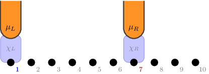
The physical system consists in a sample connected to two leads acting as particle reservoirs. We shall adopt a tight-binding description of the system: the sample is a short quantum wire and the leads are 1D and semi-infinite. In this work we consider a sample of 10 sites. This number optimizes the computational time and the physical phenomenology which we intend to describe. A sketch is given in Fig. 1. The left lead (or the source, marked as $L$ ) is contacted at one end of the sample and the right lead (or the drain, marked as $R$ ) may be contacted on any other site. The Hamiltonian of the coupled and electrically biased system reads as

H(t)=\sum_{\ell}H_{\ell}+H_{S}+H_{T}(t)=H_{0}+H_{T}(t)\,,

(1)

where $H_{S}$ is the Hamiltonian of the isolated sample, including the electron-electron interaction,

H_{S}=\sum_{n}E_{n}d_{n}^{\dagger}d_{n}+\frac{1}{2}\sum_{\begin{subarray}{c}mn\\ m^{\prime}n^{\prime}\end{subarray}}V_{mn,m^{\prime}n^{\prime}}d_{m}^{\dagger}d_{n}^{\dagger}d_{m^{\prime}}d_{n^{\prime}}\,.

(2)

The (non-interacting) single-particle basis states have wave functions $\{\phi_{n}\}$ and discrete energies $E_{n}$ . $H_{\ell}$ , with ${\{\ell\}=(L,R)}$ , is the Hamiltonian corresponding to the left and the right leads. The last term in Eq. (1), $H_{T}$ describes the time-dependent coupling between the single-particle basis states of the isolated sample and the states $\{{\psi}_{q\ell}\}$ of the leads:

H_{T}(t)=\sum_{n}\sum_{\ell}\!\int\!\mathrm{d}q\>\chi_{\ell}(t)(T^{\ell}_{qn}c^{\dagger}_{q\ell}d_{n}+\text{h.c.})\,.

(3)

The function $\chi_{\ell}(t)$ describes the time-dependent switching of the sample-lead contacts, while $d^{\dagger}_{n}$ and $c_{q\ell}$ create/annihilate electrons in the corresponding single-particle states of the sample or leads, respectively. The coupling coefficient

T^{\ell}_{qn}=V_{0}{\psi}^{*}_{q\ell}(0)\phi_{n}(i_{\ell})\,,

(4)

involves the two eigenfunctions evaluated at the contact sites $(0,i_{\ell})$ , $0$ being the site of the lead $\ell$ and $i_{\ell}$ the site in the sample [14]. In our present calculations we keep the left lead connected to the site $i_{L}=1$ , while the position of the right lead $i_{R}$ is varied. The parameter $V_{0}$ plays the role of a coupling constant between the sample and the leads.

Refer to caption — Figure 1: (Color online) A sketch of the system under study. A 1D lattice with 10 sites (“the sample”) is connected to two semi-infinite leads via tunneling. The left lead is connected to the left end of lattice, while the position of the right lead can be changed. The contacts ( $\chi_{L}$ , $\chi_{R}$ ) are modulated in time.

We will ignore the Coulomb effects in the leads, where we assume a high concentration of electrons and thus strong screening and fast particle rearrangements. The Coulomb electron-electron interaction is considered in detail only in the sample, where Coulomb blocking effects may occur. The matrix elements of the Coulomb potential in Eq. (2) are given by,

\!\!\!V_{mn,m^{\prime}n^{\prime}}=\!\int\!\mathrm{d}\vec{x}\mathrm{d}\vec{x}^{\prime}\,\phi_{m}^{*}(\vec{x})\phi_{n}^{*}(\vec{x}^{\prime})\frac{u_{C}}{|\vec{x}-\vec{x}^{\prime}|}\phi_{m^{\prime}}(\vec{x})\phi_{n^{\prime}}(\vec{x}^{\prime})\,.

(5)

We calculate the many-electron states (MES) in the sample by incorporating the Coulomb electron-electron interaction following the exact diagonalization method, i. e. without any mean field approximation. The MES are calculated in the Fock space built on non-interacting single-particle states [14]. Since the sample is open the number of electrons is not fixed, but the Coulomb interaction conserves the number of electrons. With 10 lattice sites we obtain 10 single-particle eigenstates and thus ${2^{10}=1024}$ elements in the Fock space spanned by the occupation numbers. The Coulomb effects are measured by the ratio of a characteristic Coulomb energy ${U_{C}=e^{2}/(\kappa a)}$ and the hopping energy ${t_{s}=\hbar^{2}/(2m_{\mathrm{eff}}a^{2})}$ . Here $a$ denotes the inter-site distance (the lattice constant of the discretized system), while $\kappa$ and $m_{\mathrm{eff}}$ are material parameters, the dielectric constant and the electron effective mass, respectively. In our calculations we use the relative strength of the Coulomb interaction, ${u_{C}=U_{C}/t_{s}}$ , which is treated as a free parameter.

III The transport formalism

The equation of motion for the our system is the quantum Liouville equation,

i\hbar\dot{W}(t)=\left[H(t),W(t)\right]\,,\qquad W(t<t_{0})=\rho_{L}\rho_{R}\rho_{S}\,.

(6)

$W(t)$ , the statistical operator is the solution of the equation and completely determines the evolution of the system. At times before $t_{0}$ the systems are assumed to be isolated and $W(t)$ is simply the product of the density operator of the sample and the equilibrium distributions of the leads.

Following the Nakajima-Zwanzig technique [17] we define the reduced density operator (RDO), $\rho(t)$ , by tracing out the degrees of freedom of the environment, the leads in our case, over the statistical operator of the entire system, $W(t)$

\rho(t)=\operatorname{Tr}_{L}\operatorname{Tr}_{R}W(t)\,,\qquad\rho(0)=\rho_{S}\,.

(7)

The initial condition corresponds to a decoupled sample and leads when the RDO is just the statistical operator of the isolated sample $\rho_{S}$ . For a sufficiently weak coupling strength ( $V_{0}$ ) one obtains the non-Markovian integro-differential master equation for the RDO

\begin{split}{\dot{\rho}}(t)&=-\frac{i}{\hbar}[H_{S},\rho(t)]\\ &-\frac{1}{\hbar^{2}}\sum_{\ell}\!\int\!\mathrm{d}q\>\chi_{\ell}(t)\Big(\left[{\cal T}_{q\ell},\Omega_{q\ell}(t)\right]+\text{h.c.}\Big)\,,\end{split}

(8)

where the operators $\Omega_{q\ell}$ and $\Pi_{q\ell}$ are defined as

\begin{split}\Omega_{q\ell}(t)&=e^{-itH_{S}}\!\int_{0}^{t}\!\!\mathrm{d}s\>\chi_{\ell}(s)\Pi_{q\ell}(s)e^{i(s-t)\varepsilon_{q\ell}}e^{itH_{S}}\,,\\ \Pi_{q\ell}(s)&=e^{isH_{S}}\left({\cal T}_{q\ell}^{\dagger}\rho(s)(1-f_{\ell})-\rho(s){\cal T}_{q\ell}^{\dagger}f_{\ell}\right)e^{-isH_{S}}\,,\end{split}

and $f_{\ell}$ is the Fermi function of the lead $\ell$ describing the state of the lead before being coupled to the sample. The operators ${\cal T}_{q\ell}$ and ${\cal T}_{q\ell}^{\dagger}$ describe the ’transitions’ between two many-electron states (MES) $|\alpha\rangle$ and $|\beta\rangle$ when one electron enters the sample or leaves it:

\left({\cal T}_{q\ell}\right)_{\alpha\beta}=\sum_{n}T^{\ell}_{qn}\langle\alpha|d^{\dagger}_{n}|\beta\rangle\,.

(9)

The GME is solved numerically by calculating the matrix elements of the RDO in the basis of the interacting MES, in small time steps, following a Crank-Nicolson algorithm. More details of the derivation of the GME can be found in Ref. 18. The calculation of the interacting MES is described in Ref. 14

Mean values of observables can by obtained by taking the trace of product of the corresponding operator and the RDO. The time dependent charge density is obtained from the particle-density operator, ${n(x)=\sum_{l,m}\phi_{l}^{*}(x)\phi_{m}(x)d_{l}^{\dagger}d_{m}}$ , where $\phi_{l,m}(x)$ are single-particle wave functions,

\langle Q(t,x)\rangle=\sum_{\alpha\beta}\rho_{\alpha\beta}(t)\sum_{lm}\phi_{l}^{*}(x)\phi_{m}(x)\langle\beta|d_{l}^{\dagger}d_{m}|\alpha\rangle\,.

(10)

The total time dependent charge in the sample is found by integrating over $x$ or by using the number operator ${\cal N}=\sum_{m}d_{m}^{\dagger}d_{m}$ :

\langle Q(t)\rangle=e\operatorname{Tr}\{\rho{\cal N}\}=e\sum_{N}N\sum_{\alpha_{N}}\langle\alpha_{N}|\rho(t)|\alpha_{N}\rangle\,,

(11)

where $\alpha_{N}$ denotes the (Coulomb interacting) MESs with fixed number of electrons $N$ . Remark that one can also calculate the partial charge accumulated on $N$ -particle MESs.

The currents in the system are then found by taking the derivative of Eq. (11) with respect to time,

\langle I(t)\rangle=I_{L}(t)-I_{R}(t)=e\sum_{N}N\sum_{\alpha_{N}}\langle\alpha_{N}|\dot{\rho}(t)|\alpha_{N}\rangle\,.

(12)

The time derivative of the RDO can be substituted by the right-hand side of the GME [Eq. (8)] and so it is possible identify the currents in each lead,

\begin{split}\langle I_{\ell}(t)\rangle&=-\frac{1}{\hbar^{2}}\sum_{N}N\sum_{\alpha_{N}}\int\!\mathrm{d}q\,\chi_{\ell}(t)\langle\alpha_{N}|\left[{\cal T}_{q\ell},\Omega_{q\ell}(t)\right]|\alpha_{N}\rangle\\ &+\text{h.c.}\end{split}

(13)

We also introduce a $p$ -indexed period average for the currents (the $p$ th period covers the interval [ $t_{p-1}$ , $t_{p}$ ]):

i_{p}=\frac{1}{T}\int_{\mathchoice{\hbox to0.0pt{$\displaystyle{t_{p-1}}$\hss}}{\hbox to0.0pt{$\textstyle{t_{p-1}}$\hss}}{\hbox to0.0pt{$\scriptstyle{t_{p-1}}$\hss}}{\hbox to0.0pt{$\scriptscriptstyle{t_{p-1}}$\hss}}}^{\mathchoice{\hbox to0.0pt{$\displaystyle{t_{p}}$\hss}}{\hbox to0.0pt{$\textstyle{t_{p}}$\hss}}{\hbox to0.0pt{$\scriptstyle{t_{p}}$\hss}}{\hbox to0.0pt{$\scriptscriptstyle{t_{p}}$\hss}}}\;\mathrm{d}t\>I_{\ell}(t)\,,

(14)

which in the periodic phase, i. e. sufficiently long after the initial transient stage, does not depend on $k$ and on the lead. $T$ is the period of the pulses, and $Q_{p}=Tj_{p}$ is the total charge transferred through the sample within the period $p$ .

The switching-functions in Eq. (3) act on the contact regions shaded blue in Fig. 1 and are used to mimic potential barriers with time dependent height. In the present study we use two kinds of switching-functions. The first switching-function used in the study is a sine function,

\chi_{\ell}(t)=A\Big\{1+\sin(\omega(t-s)+\phi_{\ell})\Big\}\,,

(15)

where $A=0.5$ controls the amplitude and $\omega=0.105$ the frequency. The phase shift between the leads is $\pi$ , $\phi_{L}=0$ and $\phi_{R}=\pi$ . The last parameter $s=15$ is used to shift the functions as needed.

The second switching function corresponds to quasi-rectangular pulses, and it is made by combining two quasi Fermi functions that are shifted relatively to each other,

\begin{split}\chi_{\ell}(t)=1-\frac{1}{e^{t-\gamma_{s}^{\ell}-\delta}+1}&-\frac{1}{e^{-(t-\gamma_{s}^{\ell})+(T_{p}^{\ell}+\delta)}+1}\,,\\ t&\in[0,\,2T_{p}^{\ell}]\,,\end{split}

(16)

where $\gamma_{s}^{\ell}=\{0,\,T_{p}^{L}\}$ defines the phase shift between the leads ( $\ell=L,R$ ) and $T_{p}^{\ell}=30$ is the pulse length, the same in the two leads. The pulses are not built with perfect rectangles for reasons related to numerical stability. The parameter $\delta$ controls the shape of the pulse and is fixed at the value $\delta=10$ . The time unit used is $\hbar/t_{s}$ .

The time dependent contact functions are graphed at the bottom of Figs. 7 and 3. The frequency of the functions in Eq. (15) and (16) were chosen to be similar. The initial values are $\chi_{L,R}(0)=0$ , i. e. the leads and the sample are initially disconnected.

IV Results

We will use the relative Coulomb energy ${u_{C}=1.0}$ . For a material like GaAs this value would correspond to a sample length of ${9a\approx 45}$ nm. Although quite short, this is an experimentally attainable length. We believe our results are also valid for longer samples, but the set of our parameters is also restricted by the computational time spent in solving the GME which grows very fast with the number of MES. (A typical calculation took several days of CPU.) The time unit is $\hbar/t_{s}\approx 0.029$ picoseconds. The lead-sample coupling parameter is also constant, $V_{0}=1.0$ (units of $t_{s}$ ). The chosen parameters are only optimal for the numerical approach, but they can possibly be modified to more realistic values if necessary.

IV.1 Energy spectrum

The MESs of the sample are characterized by the chemical potentials ${\mu_{N}^{(i)}:={\cal E}_{N}^{(i)}-{\cal E}_{N-1}^{(0)}}$ , where ${\cal E}_{N}^{(i)}$ is the energy of the interacting MBS number $i$ containing $N$ particles, $i=0$ indicating to the ground state and $i>0$ the excited states. In Fig. 2 we show the chemical potential diagram for our system. The strength of the Coulomb interaction is $u_{C}=1$ . For the single-particle states ( $N=1$ ) the chemical potentials are in fact the single-particle energies. The effect of the Coulomb interaction is clearly visible for $N>2$ . For example the lowest chemical potential for $N=2$ , $\mu_{2}^{(0)}\approx 2.58$ , whereas in the absence of Coulomb interaction it is equal to $\mu_{1}^{(1)}\approx 2.32$ .

We select the bias window ${\Delta\mu=\mu_{L}-\mu_{R}}$ such that it includes the ground state with $N=3$ electrons, $\mu_{L}=3.20$ and $\mu_{R}=2.98$ . The bias window includes also excited single- and two-particle states. The single-particle state is well below the top of the bias and so the population of this state will be very small, and the number of electrons in the sample is expected to be somewhere between 2 and 3. Therefore we also expect only two- and three-particle states to be involved in the transport of electrons through the sample.[14]

IV.2 Sinusoidal pulses

We begin the time-dependent calculations with $N=3$ electrons in the sample, initially assumed in the ground state. This is done by initializing the diagonal density-matrix element of the sample corresponding to this state to one and all the other matrix elements to zero. The left lead ( $L$ ) is permanently in contact with the left end of the sample, i. e. site 1. The right lead ( $R$ ) is placed on various other sites, as indicated in Fig. 1. The time evolution is then followed in short time steps, by using the contact functions $\chi_{L,R}(t)$ . The charge accumulated in the sample and the currents in the two leads are calculated at each time step. In Fig. 3 we show the results with sinusoidal pulses, corresponding to Eq. (15), and with two different placements of the $R$ lead: on sites 10 and 3.

We first observe the charge in the sample and its time evolution shown in the upper panels of Fig. 3. After the contacts begin to operate the initial charge of $N=3$ electrons changes in time. Part of the charge flows into the leads, depending on which one is accessible, and the average charge drops, until a periodic regime is established. The lower panels of the figure show the contact functions. In Fig. 3 (a) the right contact is placed at site 10. The charge in the sample has maxima and minima at the time points when the contact functions are equal. In between these time points, the charge increases when the left contact opens further and the right one closes, and decreases otherwise. The population of the three-particle and two-particle states are also shown (the population of the single-particle state being negligible) and they oscillate in antiphase, i. e. the gain of one is partly compensated by the loss of the other one.

The currents in the leads are shown in 3 (b), and they have similar shape as the contact functions, except in the initial transient phase, before the periodic regime is stabilized. In the first cycle the current in the left lead is initially negative. The sign rule is that positive currents correspond to charge flow from the left to the right lead, and negative currents correspond to the opposite direction. The initial negative current in the left lead indicates initial charge flow from the sample into that lead during the first cycle as long as the contact to the right lead is closed. The main impression of these results is that the periodic regime qualitatively corresponds to a linear response of the charge and currents to the contact strength.

The situation may change when the right contact is placed on another site, for example on site 3, as shown in 3 (c-d). In this case the oscillations of the charge and currents are weaker. The current in the left lead is no longer sinus-like. This shows now a non-linear behavior of the charge response to the same pulses as before. Some sort of standing waves are created in the sample and the right contact creates a local perturbation of the charge fluctuations at that point. Negative currents in the left lead may occur now during more pulse cycles as before. This is somewhat surprising, since such currents, although very small, are actually driven against the bias. Let’s mention that in the absence of a bias ( $\Delta\mu=0$ ) the currents in both leads oscillate between positive and negative values, but with zero average, such that no real pumping effect is obtained in this setup, irrespectively of the placement of the leads (not shown).

The currents in the leads reflect the charging or discharging of the sample, but these are actually complex processes, because different states may be occupied with different time constants, related to the tunneling matrix elements, and thus the charging and the currents may have short-time fluctuations. The fine structure of the currents is thus a complicated issue, which will be discussed further.

Before moving to that, we should remark that our charging and current curves are smooth, whereas in a real experiment the electron tunneling may look like a stochastic (discontinuous) process. Of course in this work we are not describing the electron dynamics at that level. The method of GME gives only expected values of charge and currents in the quantum mechanical sense, Eqs. (11) and (12). In the example of Fig. 3 the pulse frequency is comparable to the average tunneling rate, which is proportional to the square of the coupling parameter $V_{0}^{2}$ . But the currents are also smooth because of the sinusoidal pulses, and they will look different for rectangular pulses discussed in Section IV D.

IV.3 Charge distribution in the sample

The charge distribution inside the sample is shown in the Fig. 4 and it is far from homogeneous. The charge is averaged in time over an entire period of the contact functions when the system is in a periodic regime. In the case shown the right contact is placed on site 10. The charge distribution does not qualitatively change for other placements of the right contact (not shown). The distribution is symmetric along the sample, in spite of the presence of the bias window, which shows that the contacts between the sample and the leads are actually weak in our case. We can say that the charge distribution follows the geometrical extend of those single-particle states that contribute to the active two- and three-particle MBS.

Next, in Figs. 5 and 6, we show the deviation of the charge density from the mean value, on each lattice site, for selected time moments during half a cycle. For the other half-cycle the reverse motion occurs. The two placements of the right lead ate again selected at sites 10 and 3. Standing waves are clearly seen. For the contact configuration L1R10 (Fig. 5) the standing-wave pattern shows something between two and three wavelengths. Nodes and antinodes can be distinguished, and also a global up and down motion mode seems to occur. But it is clear that the amplitude of the charge oscillations at the contact sites is quite large.

When the right contact is on site 3 (Fig. 6) only about two wavelengths may be seen, at least for ${t<3T/8}$ , but also the charge seems to oscillate with different amplitudes at the two contacts, larger at the right lead than at the left lead. This explains the amplitudes of the currents seen in Figs. 3 (b) and (d). In other words the amplitude of the currents in the leads is related to the amplitude of the charge fluctuation at the contact. In addition, the finer structure of the current pulses reflects the existence of higher harmonics in the charge oscillations. This is suggested by the top part of Fig. 6, where we see a higher order pattern at ${t=T/2}$ than at $t=0$ .

For a better visual description of the time dependent charge oscillations we prepared a number of video files which can be accessed online, see ancillary files (Chg-osc-L1R2-sine.mp4, Chg-osc-L1R8-sine.mp4 and Chg-osc-L1R10-sine.mp4) on arXiv. The time dependent charge fluctuations and the current profiles are shown in the videos for three placements of the right leads, R2, R8, and R10, respectively. The behavior of the system shows the same symmetry as the charge distribution: the current pulses are similar when the right contact is placed on the right or on the left of the center of the sample, but at the same distance. For example R3 and R8, or R4 and R7, etc., are similar. We are seeing simple collective oscillations onset by the bias field. The counteracting (restoring) force comes from the sample-lead boundaries and from the Coulomb interaction.

IV.4 Rectangular pulses

Next we consider the more complex case of the quasi-rectangular contact functions, i. e. described by Eq. (16). Again the left lead is permanently in contact with the left end of the sample, and the right lead is placed on other sites. The representative results are shown in Fig. 7, now with four different placements of the $R$ lead: on sites 10, 7, 3, and 2, respectively. The charge evolution in time is not visibly different from the previous case of the harmonic pulses. 3 electrons, depending on the placement of the $R$ lead. The populations of the two-particle and three-particle states have opposite variations in time: the gain of one is partly compensated by the loss of the other one. It appears that the weakest charge oscillations occur when the drain lead ( $R$ ) is coupled to the site 3, like before for the sine pulses.

The calculated currents, shown in the middle panels of Fig. 7, look now more complex than those obtained for harmonic pulses. Obviously the rectangular pulses activate more higher harmonics of the charge oscillations. Still, in those cases when the amplitude of the charge oscillations is (relatively) large, i. e. when the $R$ contact is on the sites 10 and 2, the current oscillations have almost a rectangular shape, qualitatively reproducing the shape of the contact functions. After the initial irregular transient oscillations the currents become positive in both leads, describing charge propagation in the direction imposed by the the bias, i. e. from left lead to right.

The current profile is qualitatively different in the other cases, when the charge oscillations have small amplitude. Sharp and multiple oscillations are now visible in the currents, produced by higher harmonics of the charge motion, but invisible in the charge diagrams. Also, even negative currents can be seen, now in both leads, although small and only for short times, indicating again charge propagation against the bias. But now such negative currents, although weak, do not vanish in the long time limit, when the system approaches a periodic evolution in time. We thus see that the placement of the right contact is qualitatively important for the current profiles for a finite bias window. Increasing the bias window the negative currents may survive in one lead only, and further they disappear, and the current pulses take more and more the shape of the contact functions.

As for the sine pulses, the current profiles obtained for rectangular pulses obey the symmetry of the charge distribution. This means we obtain similar results for the right contact at sites 10 or 1, 9 or 2, 8 or 3, 4 or 7, and 5 or 6. Each case is shown in Fig. 7 once, except the later two, R5 and R6, which actually look qualitatively similar to R10, only slightly sharper.

In order to observe better the effects of higher harmonics of the charge oscillations we show in Fig. 8 and Fig. 9 the Fourier analysis for two selected contact configurations of rectangular pulses, L1R10 and L1R3 respectively. Figs. 8 (a) and 9 (a) show the Fourier components of the switching-function $\chi_{\ell}(t)$ in Eq. (16). The current approximately follows the pulse shape in the left lead when contacts are placed at L1R10 (Fig. 8 (c)). This behavior is not seen in the right lead (Fig. 8 (d)) or when the contacts are placed at L1R3 (Fig. 9 (c-d)). The Fourier components of the total charge are shown in Figs. 8 (b) and 9 (b). The first harmonic is the most dominant for the configuration L1R10, but for L1R3 (see Fig. 9) the cumulative contribution of higher harmonics is almost comparable to the main component.

IV.5 Charge propagation

Next we discuss the amount of charge which propagates through the sample during one period by our simulated turnstile pump, $Q_{k}=TI_{k}$ , where $k$ is the right contact site and $I_{k}$ the current averaged over one pulse period, from $t\approx 280$ to $t\approx 340$ . This is shown in Fig. 10 where we compare the results for the two type of pulses. Interestingly, the pumped charge increases for rectangular pulses. This happens especially for those contact locations which produce quasi-rectangular currents, 1, 2, 5, 6, 8, 10. This can be attributed to higher harmonics of the charge oscillations.

Until now all results have been obtained for a fixed frequency of the contact pulses $T=60$ time units, which correspond to an angular frequency ${\omega=2\pi/T\approx 0.105}$ . In Fig. 11 we show the average current (which gives the transferred charge) for a variable frequency, in the interval 0.05-0.2. The curve is smooth, but the maximum current is obtained for a frequency between 0.11-0.15. The frequency corresponding to the maximum current can be related to the energy spectrum, Fig. 2. The bias window includes the two-particle and three-particle states with chemical potentials ${\mu_{2}^{(2)}=3.231}$ and ${\mu_{3}^{(0)}=3.344}$ . The difference between these values, 0.113, is in the frequency interval containing the maximum current, which in fact describes a resonance between two- and three-particle states. The resonance is broad because of the effect of the contacts in the electron states in the sample. The strength of the lead-sample coupling $|V_{0}T_{qn}^{l}|^{2}$ is of the order 0.02 in our calculations. At larger frequencies (larger than 0.18) the pulses become to fast so the charge in the sample cannot follow the imposed time evolution, and so the current drops.

Finally, in Fig. 12 we show again the deviation of the charge density from the mean value, i. e. the standing waves, for two frequencies different from the frequency used in Section IV B-D ( $\omega=0.105$ ). In Fig. 12 (a) the frequency of the switching-function in Eq. 15 has been lowered to ${\omega=0.05}$ while in Fig. 12 (a) it has been raised to ${\omega=0.20}$ . The standing-waves observed are qualitatively similar to those seen in Figs. 5 for ${\omega=0.05}$ , although of a slightly smaller amplitude, for example at $T/8$ , which is consistent with Fig. 11. For ${\omega=0.20}$ we find the higher modes attenuated and apparently a longer wavelength. However, a systematic investigation of the dispersion of the standing waves is not possible at this stage.

V Concluding remarks

We have simulated the time dependent transport through a one-dimensional interacting finite quantum wire attached to two leads, described by a lattice model. Out-of-phase time periodic signals are applied at the contact sites generating a turnstile operation. The calculations are performed by solving the generalized master equation of the reduced density operator in the Fock space of the many-body states of the electrons in the sample, which are calculated via exact diagonalization. The time periodic contacts generate standing waves of charge along the length of the wire with finer details depending on the location of the contacts. The amplitude of the currents depends on the contact site not only through the tunneling constants but also through the amplitude of the charge fluctuations at the given contact. The current profile in the leads is determined by the charge fluctuations in the sample, which depend on the entire standing wave pattern. We have called this model a quantum flute.

We emphasize that the excitation of these collective oscillations are obtained from a fully quantum treatment of an open few-electron system. Collective oscillations have been studied in quantum dots with few electrons by mapping out the oscillator strength of exact MESs [19] or a by more traditional linear response approach [20]. The evolution to systems with a higher number of electrons has also been studied [21]. In the present work the excitation method is of a different type and it may be used in transport measurements.

The charge oscillations occur both due to the finite length of the sample and due to the Coulomb interaction. Both the boundaries of the sample and the Coulomb repulsion create the restoring (“elastic”) forces. The Coulomb interaction has also an important role in the charge distribution, through the well known blocking and correlation effects, and therefore the inclusion of the Coulomb effects is necessary for a consistent description. The relative strength of the Coulomb interaction $u_{C}$ may however depends on the material constants. It is quite difficult to compare the results without and with the Coulomb interaction included for the same set of parameters (i. e. bias window, coupling constants). If Coulomb effects are neglected ( $u_{C}=0$ ) the whole energy spectrum changes and new states are present within the bias window. Then the chemical potentials in the leads have to be shifted accordingly in order to capture in the bias window states with similar number of electrons as in the interacting case. This means one cannot compare the two situations just by changing only one parameter.

Our calculations are performed for a relatively weak coupling of the sample to leads. In this case the perturbation of the sample states due to the leads is minimal, and so the results can still be interpreted in terms of the states of the sample itself. Increasing the coupling strength the finer details of the current profile determined by the sample may be washed out.

The standing waves are obviously not possible in quantum dots where, to our knowledge, most of the experimental and theoretical work on turnstile pumping has been done. Therefore the spatial extension of the sample is, in our opinion, a novel element in this topic. The short time scale of the oscillations, in the picosecond domain, is related to the energy gaps between the quantum states. This domain is attainable by the present experimental technology.

In this work we completely ignored the Coulomb interaction in the leads. Due to computational limitations we studied a short nanowire which generated a short time scale. And also a relatively narrow bias window, which together with the weak sample-leads coupling yielded low currents. But even though the currents calculated in these examples are small and we are limited here only to the qualitative effects, the predicted results may be seen in future experiments. For example in a setup with an array of finger electrodes placed on top of a single wire where currents can be driven by any pair of contacts [22, 23]. Another possibility is to change the location of one contact, like in our simulations, using a scanning tunneling or a conductive atomic force microscope [24]. Consequently one can expect that a suitable placement of the source and drain leads along the sample would be a way to deliver modulated output currents with a desired shape and period. The time dependent charge propagation along transmission lines of a quantum mechanical nature may be a future direction in the field of nanophysics.

Acknowledgements.

This work was financially supported by the Icelandic Research Fund. V.M. was also supported by the grant of the Romanian National Authority for Scientific Research, CNCS – UEFISCDI, project number PN-II-ID-PCE-2011-3-0091.

References

[1] T. Fujisawa, D. G. Austing, Y. Tokura, Y. Hirayama, and S. Tarucha, Journal of Physics: Condensed Matter 15, R1395 (2003).
[2] B. Naser, D. K. Ferry, J. Heeren, J. L. Reno, and J. P. Bird, Applied Physics Letters 89, 083103 (2006).
[3] B. Naser, D. K. Ferry, J. Heeren, J. L. Reno, and J. P. Bird, Applied physics letters 90, 043103 (2007).
[4] W.-T. Lai, D. M. Kuo, and P.-W. Li, Physica E 41, 886 (2009).
[5] A. Fuhrer, C. Fasth, and L. Samuelson, Applied Physics Letters 91, 052109 (2007).
[6] B. Kaestner, V. Kashcheyevs, S. Amakawa, M. D. Blumenthal, L. Li, T. J. B. M. Janssen, G. Hein, K. Pierz, T. Weimann, U. Siegner, and H. W. Schumacher, Phys. Rev. B 77, 153301 (2008).
[7] S. Kurth, G. Stefanucci, C.-O. Almbladh, A. Rubio, and E. K. U. Gross, Phys. Rev. B 72, 035308 (2005).
[8] P. Myöhänen, A. Stan, G. Stefanucci, and R. van Leeuwen, Phys. Rev. B 80, 115107 (2009).
[9] A. R. Hernández, F. A. Pinheiro, C. H. Lewenkopf, and E. R. Mucciolo, Phys. Rev. B 80, 115311 (2009).
[10] C. M. Gainar, V. Moldoveanu, A. Manolescu, and V. Gudmundsson, New Journal of Physics 13, 013014 (2011).
[11] L. P. Kouwenhoven, A. T. Johnson, N. C. van der Vaart, C. J. P. M. Harmans, and C. T. Foxon, Phys. Rev. Lett. 67, 1626 (1991).
[12] Y. Mizugaki, Journal of applied physics 94, 4480 (2003).
[13] H. Ikeda and M. Tabe, Journal of applied physics 99, 073705 (2006).
[14] V. Moldoveanu, A. Manolescu, C.-S. Tang, and V. Gudmundsson, Phys. Rev. B 81, 155442 (2010).
[15] J. Splettstoesser, M. Governale, J. König, and R. Fazio, Phys. Rev. Lett. 95, 246803 (2005).
[16] E. Sela and Y. Oreg, Phys. Rev. Lett. 96, 166802 (2006).
[17] C. Timm, Phys. Rev. B 77, 195416 (2008).
[18] V. Moldoveanu, A. Manolescu, and V. Gudmundsson, New Journal of Physics 11, 073019 (2009).
[19] D. Pfannkuche and R. R. Gerhardts, Phys. Rev. B 44, 13132 (1991).
[20] V. Gudmundsson and R. R. Gerhardts, Phys. Rev. B 43, 12098 (1991).
[21] D. Pfannkuche, V. Gudmundsson, P. Hawrylak, and R. Gerhardts, Solid-State Electronics 37, 1221 (1994).
[22] R. Frielinghaus, S. Estévez Hernández, R. Calarco, and Th. Schäpers, Appl. Phys. Lett. 94, 252107 (2009).
[23] C. Blömers, J. G. Lu, L. Huang, C. Witte, D. Grützmacher, H. Lüth, and T. Schäpers, Nano Lett., DOI: 10.1021/nl204500r, Publication Date (Web): April 11, 2012.
[24] X. Zhou, S. A. Dayeh, D. Aplin, D. Wang, and E. T. Yu, Appl. Phys. Lett. 89, 053113 (2006).