High-Dimensional Feature Selection by Feature-Wise Kernelized Lasso
Abstract
The goal of supervised feature selection is to find a subset of input features that are responsible for predicting output values. The least absolute shrinkage and selection operator (Lasso) allows computationally efficient feature selection based on linear dependency between input features and output values. In this paper, we consider a feature-wise kernelized Lasso for capturing non-linear input-output dependency. We first show that, with particular choices of kernel functions, non-redundant features with strong statistical dependence on output values can be found in terms of kernel-based independence measures such as the Hilbert-Schmidt independence criterion (HSIC). We then show that the globally optimal solution can be efficiently computed; this makes the approach scalable to high-dimensional problems. The effectiveness of the proposed method is demonstrated through feature selection experiments for classification and regression with thousands of features.
1 Introduction
Finding a subset of features in high-dimensional supervised learning is an important problem with many real-world applications such as gene selection from microarray data (Xing et al., 2001; Ding and Peng, 2005; Suzuki et al., 2009; Huang et al., 2010), document categorization (Forman, 2008), and prosthesis control (Shenoy et al., 2008).
1.1 Problem Description
Let be the domain of input vector and be the domain of output data11 1 could be either continuous (i.e., regression) or categorical (i.e., classification). Structured outputs can also be handled in our proposed methods. . Suppose we are given independent and identically distributed (i.i.d.) paired samples,
drawn from a joint distribution with density . We denote the original data by
where ⊤ denotes the transpose.
The goal of supervised feature selection is to find features () of input vector that are responsible for predicting output .
1.2 Lasso
The least absolute shrinkage and selection operator (Lasso) (Tibshirani, 1996) allows computationally efficient feature selection based on the assumption of linear dependency between input features and output values.
The Lasso optimization problem is given as
where is a regression coefficient vector, denotes the regression coefficient of the -th feature, and are the - and -norms, and is the regularization parameter. The -regularizer in Lasso tends to produce a sparse solution, which means that the regression coefficients for irrelevant features become zero. Lasso is particularly useful when the number of features is larger than the number of training samples (Tibshirani, 1996). Furthermore, various optimization software packages were developed for efficiently computing the Lasso solution (Boyd and Vandenberghe, 2004; Daubechies et al., 2004; Combettes and Wajs, 2005; Kim et al., 2007; Yin et al., 2008; Wright et al., 2009; Tomioka et al., 2011).
However, a critical limitation of Lasso is that it cannot capture non-linear dependency.
1.3 Instance-Wise Non-Linear Lasso
To handle non-linearity, the instance-wise non-linear Lasso was introduced (Roth, 2004), where the original instance is transformed by a non-linear function . Then the Lasso optimization problem is expressed as
where , is a regression coefficient vector, and is a coefficient of the -th basis .
The instance-wise non-linear Lasso gives a sparse solution in terms of instances, but not features. Therefore, it cannot be used for feature selection.
1.4 Feature-Wise Non-Linear Lasso (Feature Vector Machine)
To obtain sparsity in terms of features, the feature-wise non-linear Lasso was proposed (Li et al., 2006).
The key idea is to apply a non-linear transformation in a feature-wise manner, not in an instance-wise manner. More specifically, let us represent the sample matrix in a feature-wise manner as
where is the vector of the -th feature for all samples. Then the feature vector and the output vector are transformed by a non-linear function . The Lasso optimization problem in the transformed space is given as
| (1) |
where is a regression coefficient vector and denotes the regression coefficient of the -th feature. By using the kernel trick (Schölkopf and Smola, 2002), Eq.(1) was shown to be equivalently expressed as the following quadratic programming (QP) problem:
| s.t. | (2) |
where and . This formulation is called the feature vector machine (FVM). Note, since FVM uses dimensional Hessian matrix , it is especially useful when the number of training samples is much bigger than that of features .
In the original FVM, mutual information (Cover and Thomas, 2006) was used as the kernel function . However, the matrix obtained from mutual information is not necessarily positive definite (Seeger, 2002), and thus the objective function Eq.(2) can be non-convex. Furthermore, when the number of training samples is smaller than that of features (which is often the case in high-dimensional feature selection scenarios), the matrix is singular. This can cause numerical instability. Another restriction of FVM is that, irrespective of regression or classification, output should be transformed by the same non-linear function as feature vector . This highly limits the flexibility of capturing non-linear dependency. Finally, it is not statistically clear what kind of features are found by this FVM formulation.
1.5 Contribution of This Paper
To overcome the limitations of FVM, we propose an alternative feature-wise non-linear Lasso. More specifically, we propose to use particular forms of universal reproducing kernels (Steinwart, 2001) as feature and output transformations, and solve the optimization problem in the primal space.
An advantage of this new formulation is that the global optimal solution can be computed efficiently. Thus, it is scalable to high-dimensional feature selection problems. To the best of our knowledge, this is the first convex feature selection method that is able to deal with high-dimensional non-linearly related features. Furthermore, this new formulation has a clear statistical interpretation that non-redundant features with strong statistical dependence on output values are found via kernel-based independence measures such as the Hilbert-Schmidt independence criterion (HSIC) (Gretton et al., 2005) and the criterion based on the normalized cross-covariance operator (NOCCO) (Fukumizu et al., 2008). Thus, the proposed methods can be regarded as a minimum redundancy maximum relevance based feature selection method (Peng et al., 2005). In addition, the proposed methods are simple to implement, which is a highly preferable property for practitioners.
We also discuss the relation between the proposed method and existing feature selection approaches such as minimum redundancy maximum relevance (mRMR) (Peng et al., 2005), HSIC-based greedy feature selection (Song et al., 2012), quadratic programming feature selection (QPFS) (Rodriguez-Lujan et al., 2010), kernel target alignment (KTA) (Shawe-Taylor and Kandola, 2002; Cortes et al., 2012), Hilbert-Schmidt Feature Selection (HSFS) (Masaeli et al., 2010), and sparse additive models (SpAM) (Ravikumar et al., 2009; Liu et al., 2009; Raskutti et al., 2012). See Table 1 for the summary of feature selection methods.
| Method | Dependency | Optimization | Primal/Dual | Scalability w.r.t. | Structured output |
|---|---|---|---|---|---|
| # of features | |||||
| Lasso | Linear | Convex | Primal | Highly scalable | Not available |
| mRMR | Non-linear | Greedy | — | Scalable | Available |
| Greedy HSIC | Non-linear | Greedy | — | Scalable | Available |
| HSFS | Non-linear | Non-convex | — | Not scalable | Available |
| FVM | Non-linear | Non-convex† | Dual | Not scalable | Available |
| QPFS/KTA | Non-linear | Non-convex† | Dual | Not scalable | Available |
| SpAM | Additive non-linear | Convex | Primal | Scalable | Not available |
| Proposed | Non-linear | Convex | Primal | Highly scalable | Available |
†In practice, positive constants may be added to the diagonal elements of the Hessian matrix to guarantee the convexity, although the validity of selected features by this modification is not statistically clear.
Through experiments on real-world feature selection problems, we show that the proposed methods compare favorably with existing feature selection methods.
2 Proposed Methods
In this section, we propose alternative implementations of the non-linear feature-wise Lasso.
2.1 HSIC Lasso
We propose a feature-wise non-linear Lasso of the following form, which we call the HSIC Lasso22 2 A MATLAB® implementation of the proposed algorithm is available from http://www.makotoyamada-ml.com/hsiclasso.html.:
| s.t. | (3) |
where is the Frobenius norm, and are centered Gram matrices, and are Gram matrices, and are kernel functions, is the centering matrix, is the -dimensional identity matrix, and is the -dimensional vector with all ones. Note that we employ non-negativity constraint for so that meaningful features are selected (see Section 2.2 for details). In addition, since we use the output Gram matrix to select features in HSIC Lasso, we can naturally incorporate structured outputs via kernels. Moreover, we can perform feature selection even if the training data set consists of input and its affinity information such as link structures between inputs.
2.2 Interpretation of HSIC Lasso
Here, we show that HSIC Lasso can be regarded as a minimum redundancy maximum relevancy (mRMR) based feature selection method (Peng et al., 2005), which is a popular feature selection strategy in machine learning and artificial intelligence communities.
The first term in Eq.(3) can be rewritten as
| (4) |
where is a kernel-based independence measure called the (empirical) Hilbert-Schmidt independence criterion (HSIC) (Gretton et al., 2005) and denotes the trace. is a constant and can be ignored. HSIC always takes a non-negative value, and is zero if and only if two random variables are statistically independent when a universal reproducing kernel (Steinwart, 2001) such as the Gaussian kernel is used. Note that the empirical HSIC asymptotically converges to the true HSIC with (see Theorem 3 in Gretton et al. (2005)). In addition, HSIC can be regarded as the centered version of the kernel target alignment (KTA) (Shawe-Taylor and Kandola, 2002).
If the -th feature has high dependence on output , takes a large value and thus should also take a large value so that Eq.(3) is minimized. On the other hand, if is independent of , is close to zero and thus such tends to be eliminated by the -regularizer. This means that relevant features that have strong dependence on output tend to be selected by HSIC Lasso.
Furthermore, if and are strongly dependent (i.e., redundant features), takes a large value and thus either of and tends to be zero. This means that redundant features tend to be eliminated by HSIC Lasso.
Overall, HSIC Lasso tends to find non-redundant features with strong dependence on output , which is the idea of minimum redundancy maximum relevancy (mRMR) based feature selection methods (Peng et al., 2005). This is a preferable property in feature selection.
Note that, it is possible to remove the non-negativity constraint in Eq.(3) and select features that have non-zero coefficients . However, if we allow negative values in , it is hard to interpret selected features. Indeed, interpretability is one of important properties in feature selection, and thus we include the non-negativity constraint for HSIC Lasso.
2.3 Kernel Selection
In theory, a universal kernel such as the Gaussian kernel or the Laplace kernel permits HSIC to detect dependence between two random variables (Gretton et al., 2005). Moreover, it has been proposed to use the delta kernel for multi-class classification problems (Song et al., 2012). Thus, in this paper, we employ the Gaussian kernel for inputs. For output kernels, we use the Gaussian kernel for regression cases and the delta kernel for classification problems.
For input , we first normalize the input to have unit standard deviation, and we use the Gaussian kernel:
where is the Gaussian kernel width.
In regression scenarios (i.e., ), we normalize an output to have unit standard deviation, and we use the Gaussian kernel:
where is the Gaussian kernel width.
In classification scenarios (i.e., is categorical), we use the delta kernel for ,
where is the number of samples in class . Note that it is also possible to use the Gaussian kernel in classification scenarios, but it tends to perform poorly (see Figure 4).
2.4 Computational Properties of HSIC Lasso
An important computational property of HSIC Lasso is that the first term in Eq.(3) can be rewritten as
where is the vectorization operator. This is the same form as plain Lasso with samples and features.
If (i.e., high-dimensional feature selection from a small number of training samples), the Lasso optimization technique called the dual augmented Lagrangian (DAL)33 3 http://www.ibis.t.u-tokyo.ac.jp/ryotat/dal/ was shown to be computationally highly efficient (Tomioka et al., 2011). Because DAL can also incorporate the non-negativity constraint without losing its computational advantages, we can directly use DAL to solve our HSIC Lasso problem. In contrast, when , we may use the either cKTM or FVM (i.e., dual) formulation.
If the number of samples is relatively large, the Gaussian kernel computation in HSIC Lasso is expensive. Therefore, the overall computation cost of HSIC Lasso is high. In addition, since naive implementation of HSIC Lasso requires memory space, it is not practical if both and are large (e.g., and ). Here, we propose a table lookup approach to reduce the computation time and memory size.
More specifically, based on the fact that the Gaussian kernel values depend only on the difference of two input values, we normalize every feature to have mean zero and unit standard deviation and discretize the difference of two input values into values (we use in our implementation). Then, we prepare in advance a lookup table of elements that contain Gaussian kernel values and refer to these values when we compute the Gaussian kernels. The centered Gram matrix can be rewritten as
where and . Thus, to compute , we only need to store and . Namely, the required memory size for the table lookup based approach is , which is much smaller than the memory size required for the naive implementation, .
Another approach to deal with large sample size would be using stability selection which consists in running HSIC Lasso many times with subsampling and computing the number of times each feature is selected across the runs (Meinshausen and Bühlmann, 2010; Bach, 2008).
2.5 Variation: NOCCO Lasso
Instead of and , let us use and , where is a regularization parameter. Then our optimization problem is expressed as
| s.t. |
where is the kernel-based dependence measure based on the (empirical) normalized cross-covariance operator (NOCCO) (Fukumizu et al., 2008). We call this formulation the NOCCO Lasso.
Because was shown to be asymptotically independent of the choice of kernels, NOCCO Lasso is expected to be less sensitive to the kernel parameter choice than HSIC Lasso, although needs to be tuned in practice.
2.6 Other Types of Regularizers
The proposed method is amenable to most of the popular regularizers such as group-lasso and elastic-net regularizers (Meier et al., 2008; Zou and Hastie, 2005), as well as to other feature selection problems. For example, the group-lasso regularizer can be easily incorporated into our framework as
| s.t. |
where , is the th group of variables, and is the number of groups. This group-lasso problem can also be efficiently solved by the DAL package with the non-negativity constraint.
2.7 Relation to Two-Stage Multiple Kernel Learning
The proposed method is closely related to the two-stage multiple kernel learning (MKL) method called centered kernel target alignment (cKTA) (Cortes et al., 2012), which has been originally proposed for learning a kernel Gram matrix (not used for feature selection problems).
If we adopt cKTA for supervised feature selection problems, the optimization problem of cKTA can be written as
| s.t. |
Differences from the HSIC Lasso are that cKTA solve the optimization problem in the dual space and does not have the regularization term.
An advantage of cKTA is that feature selection can be performed just by solving a non-negative least-squares problem. Moreover, since cKTA has dimensional Hessian matrix (), cKTA is computationally efficient for feature selection problems with large and small . However, the Hessian matrix is not necessarily positive definite (Seeger, 2002) and is singular in high-dimensional problems. More specifically, can be written as
and is singular when (i.e., high-dimensional feature selection from a small number of training samples). Thus, solving the non-negative least-squares problem in high-dimensional feature selection problems can be cumbersome in practice.
For the above reason, the proposed feature selection method is more suited than cKTA for high-dimensional feature selection problems. In contrast, if we want to solve a small and large feature selection problem, cKTA is more suited than the HSIC Lasso.
3 Existing Methods
In this section, we review existing feature selection methods and discuss their relation to the proposed approach. See Table 1 for the summary of feature selection methods.
3.1 Minimum Redundancy Maximum Relevance (mRMR)
Minimum redundancy maximum relevance (mRMR) (Peng et al., 2005) is a mutual information based feature selection criterion.
Let be a sub-matrix of , where features are extracted from features. Then mRMR for is defined as follows:
| (6) |
where is an empirical approximator of mutual information given as
denotes a Parzen window estimator of the joint density of and , and and denotes Parzen window estimators of marginal densities of and , respectively.
The first term in mRMR measures the dependency between chosen feature and output , while the second term is a penalty for selecting redundant features. Thus, mRMR finds non-redundant features with strong dependence on outputs. A very fast implementation of mRMR available, and thus, it can deal with high-dimensional feature selection problems.
mRMR-based feature selection is performed by finding a sub-matrix that maximizes Eq.(6). However, since there are possible feature subsets, the brute force approach is computationally intractable. Hence, greedy search strategies such as forward selection/backward elimination are used in practice (Peng et al., 2005). However, the greedy approaches tend to produce a locally optimal feature set.
Another potential weakness of mRMR is that mutual information is approximated by Parzen window estimation—Parzen window based mutual information estimation is unreliable when the number of training samples is small (Suzuki et al., 2009).
3.2 Greedy Feature Selection with HSIC
The HSIC-based feature selection criterion (Song et al., 2012) is defined as
| (7) |
where is a centered Gram matrix, is a Gram matrix, is a kernel function, and .
HSIC-based greedy feature selection is performed by finding a sub-matrix that maximizes Eq.(7). An advantage of HSIC-based feature selection is its simplicity; it can be implemented very easily. However, since the maximization problem Eq.(7) is NP-hard, forward selection/backward elimination strategies are used for finding a locally optimal solution in practice (Song et al., 2012).
3.3 Hilbert-Schmidt Feature Selection (HSFS)
Hilbert-Schmidt feature selection (HSFS) (Masaeli et al., 2010) is defined as
where is a transformation matrix, is the regularization parameter, and is the -norm.
HSFS can be regarded as a continuously relaxed version of the HSIC-based feature selection (Song et al., 2012). Thanks to this continuous formulation, the HSFS optimization problem can be solved by limited-memory BFGS (L-BFGS) (Nocedal and Wright, 2003). However, since HSFS is a non-convex method, restarting from many different initial points would be necessary to select good features, which is computationally expensive. Moreover, HSFS attempts to optimize a projection matrix which has parameters. That is, following the original HSFS implementation based on a Quasi-Newton method, the total computational complexity of HSFS is , which can be unacceptably large in high-dimensional feature selection problems. To reduce the computational cost, it may be able to approximately solve the HSFS optimization problem by reducing the size of the transformation matrix to for . However, this approximation leads to an additional tuning parameter that can not be chosen objectively.
3.4 Quadratic Programming Feature Selection (QPFS)
Quadratic programming feature selection (QPFS) (Rodriguez-Lujan et al., 2010) tries to find features by solving a QP problem.
The QPFS optimization problem is defined as
| s.t. |
where , , , is a dependency measure, and is a tuning parameter. In QPFS, an empirical estimator of mutual information is used as a dependency measure. Note that if we employ HSIC as a dependency measure in QPFS and remove the sum-to-one constraint, QPFS is equivalent to the centered KTA (cKTA) (Cortes et al., 2012), which is a multiple kernel learning method and has been originally proposed for learning a kernel matrix (see Section 2.7 for details).
Similar to cKTA, an advantage of QPFS is that feature selection can be performed just by solving a QP problem. Moreover, since QPFS has dimensional Hessian matrix, QPFS is computationally efficient for feature selection problems with large and small . However, the Hessian matrix is not necessarily positive definite (Seeger, 2002) and is singular in high-dimensional problems.
3.5 Sparse Additive Models (SpAM)
The sparse additive models (SpAM) is useful for high-dimensional feature selection (Ravikumar et al., 2009; Liu et al., 2009; Raskutti et al., 2012; Suzuki and Sugiyama, 2013).
The SpAM optimization problem can be expressed as
where are regression coefficient vectors, is a coefficient for , and is a regularization parameter. This problem can be efficiently solved by the back-fitting algorithm (Ravikumar et al., 2009). Note that SpAM is closely related to the hierarchical multiple kernel learning (Bach, 2009), which employs a sparse additive model with an alternative sparsity-inducing regularizer.
An advantage of SpAM is that it is a convex method and can be efficiently optimized by the backfitting algorithm. Moreover, statistical properties of the SpAM estimator are well studied (Ravikumar et al., 2009). A potential weakness of SpAM is that it can only deal with additive models. That is, if data follows a non-additive model, SpAM may not work well (see Figure 1(b)). Another weakness of SpAM is that it needs to optimize variables, while the proposed methods contain only variables. Thus, SpAM optimization tends to be computationally more expensive than the proposed methods. Finally, an output should be a real number in SpAM, meaning that SpAM cannot deal with structured outputs such as multi-label and graph data.
4 Experiments
In this section, we experimentally investigate the performance of the proposed and existing feature selection methods using synthetic and real-world datasets.
4.1 Setup
We compare the performance of the proposed methods with mRMR (Peng et al., 2005), QPFS (Rodriguez-Lujan et al., 2010), cKTA (Cortes et al., 2012), forward selection with HSIC (FHSIC), FVM (Li et al., 2006), and SpAM44 4 We thank the authors of (Ravikumar et al., 2009) for providing us the code used in their paper. (Ravikumar et al., 2009). Note that, since it has been reported that the performance of FHSIC is comparable to HSFS and HSFS is computationally expensive for high-dimensional data, we decided to only compare the proposed method to FHSIC. For FVM, QPFS, and mRMR, the C++ implementation of a mutual information estimator55 5 http://penglab.janelia.org/proj/mRMR/ is used. Then, a QP solver SeDuMi66 6 http://sedumi.ie.lehigh.edu/ is used to solve the FVM and QPFS optimization problems. We observed that the matrices in FVM, QPFS, and cKTA tend not to be positive definite. In our experiments, we added a small constant to the diagonal elements of so that the objective function becomes convex. For all experiments, we set in FVM, in QPFS and cKTA, and in NOCCO Lasso. For proposed methods, we experimentally use .
4.2 Synthetic Datasets
First, we illustrate the behavior of the proposed HSIC Lasso and NOCCO Lasso using the following two synthetic datasets:
- (a) Data1 (Additive model):
-
where and . Here, denotes the multi-variate Gaussian distribution with mean and covariance matrix .
- (b) Data2 (Non-additive model):
-
where and .

(a) Data1 (Additive model)

(b) Data2 (Non-additive model)

(c) Computation time for Data2

(d) Computation time of HSIC Lasso for Data2
Figure 1 shows the feature selection accuracy of each method over 30 runs as functions of the number of samples, where the accuracy is measured by the fraction of correctly selected features under the assumption that the number of true features is known. As the figure clearly shows, the proposed HSIC Lasso and NOCCO Lasso methods select good features in both additive and non-additive model cases. SpAM also works very well for Data1, but it performs poorly for Data2 because the additivity assumption is violated in Data2. QPFS and FVM behave similarly, but they tend to be outperformed by the proposed methods.
Next, we compare the computation time of each method. Here, we change the number of features in Data2 to , while we fix the number of samples to . Figure 1-(c) shows the average computation time for each method over runs. As can be observed, the computation time of HSIC Lasso and NOCCO Lasso increases mildly with respect to the number of features compared to that of SpAM, FVM, and QPFS. Figure 1-(d) shows the average computation time of HSIC Lasso for runs. In this experiment, we use the table lookup trick for HSIC Lasso to deal with a relatively large number of samples. This shows that the lookup trick allows us to handle relatively large datasets.
4.3 Real-World Datasets
Next, we compare the performance of feature selection methods using real-world datasets.
4.3.1 Multi-Class Classification
We use four image datasets and two microarray datasets77 7 http://featureselection.asu.edu/datasets.php. Detailed information of the datasets is summarized in Table 2.
| Type | Dataset | # features () | # samples () | # Classes |
|---|---|---|---|---|
| Image | AR10P | 2400 | 130 | 10 |
| PIE10P | 2400 | 210 | 10 | |
| PIX10P | 10000 | 100 | 10 | |
| ORL10P | 10000 | 100 | 10 | |
| Microarray | TOX | 5748 | 171 | 4 |
| CLL-SUB | 11340 | 111 | 3 |
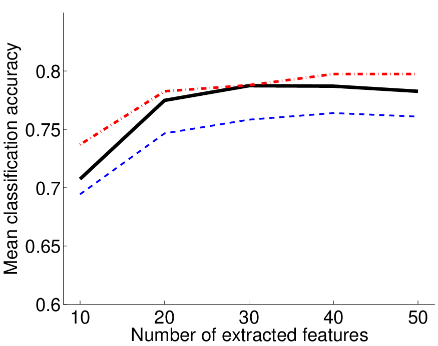
In this experiment, we use 80 of samples for training and the rest for testing. We repeat the experiments 100 times by randomly shuffling training and test samples, and evaluate the performance of feature selection methods by the average classification accuracy. We use multi-class -regularized kernel logistic regression (KLR) (Hastie et al., 2001; Yamada et al., 2010) with the Gaussian kernel for evaluating the classification accuracy when the top features selected by each method are used. In this paper, we first choose 50 features and then use top features having the largest absolute regression coefficients. In KLR, all tuning parameters such as the Gaussian width and the regularization parameter are chosen based on 3-fold cross-validation.
We also investigate the redundancy rate (RED) (Zhao et al., 2010)88 8 The original redundancy rate was defined with a plain correlation coefficient (Pearson, 1920), not the absolute correlation coefficient (Zhao et al., 2010). However, this is not appropriate as an error metric because negative correlation decreases RED. For this reason, we decided to use the absolute correlation coefficient.,
where is the correlation coefficient between the -th and -th features. A large RED score indicates that selected features are more strongly correlated to each other, that is, many redundant features are selected. Thus, as a feature selection method, a small redundancy rate is preferable.

(a) AR10P

(b) PIE10P

(c) PIX10P

(d) ORL10P

(e) TOX

(f) CLL-SUB
| Dataset | HSIC | NOCCO | SpAM | FVM | mRMR | QPFS | cKTA | FHSIC | ||||||||
|---|---|---|---|---|---|---|---|---|---|---|---|---|---|---|---|---|
| Lasso | Lasso | |||||||||||||||
| AR10P | .848 | (.111) | .846 | (.111) | .551 | (.109) | .795 | (.121) | .745 | (.136) | .743 | (.137) | .709 | (.207) | .773 | (.122) |
| PIE10P | .971 | (.032) | .972 | (.031) | .898 | (.109) | .955 | (.062) | .895 | (.118) | .952 | (.067) | .884 | (.218) | .908 | (.091) |
| PIX10P | .964 | (.043) | .964 | (.042) | .857 | (.146) | — | (—) | .769 | (.124) | .924 | (.067) | .920 | (.090) | .920 | (.100) |
| ORL10P | .938 | (.068) | .941 | (.066) | .669 | (.120) | — | (—) | .782 | (.138) | .884 | (.096) | .848 | (.140) | .788 | (.132) |
| TOX | .781 | (.119) | .788 | (.113) | .691 | (.087) | .686 | (.085) | .709 | (.084) | .769 | (.077) | .804 | (.110) | .715 | (.087) |
| CLL-SUB | .768 | (.087) | .769 | (.084) | .524 | (.112) | — | (—) | .640 | (.098) | .760 | (.116) | .709 | (.104) | .732 | (.141) |
| Dataset | HSIC | NOCCO | SpAM | FVM | mRMR | QPFS | cKTA | FHSIC | ||||||||
|---|---|---|---|---|---|---|---|---|---|---|---|---|---|---|---|---|
| Lasso | Lasso | |||||||||||||||
| AR10P | .196 | (.028) | .195 | (.028) | .255 | (.036) | .260 | (.039) | .268 | (.038) | .217 | (.050) | .235 | (.034) | .350 | (.091) |
| PIE10P | .135 | (.014) | .139 | (.017) | .250 | (.042) | .193 | (.029) | .225 | (.036) | .183 | (.026) | .155 | (.021) | .285 | (.059) |
| PIX10P | .177 | (.023) | .174 | (.023) | .388 | (.105) | — | (—) | .200 | (.066) | .286 | (.057) | .198 | (.036) | .348 | (.064) |
| ORL10P | .192 | (.026) | .191 | (.025) | .300 | (.047) | — | (—) | .294 | (.095) | .204 | (.032) | .191 | (.034) | .225 | (.045) |
| TOX | .382 | (.027) | .381 | (.027) | .391 | (.028) | .422 | (.031) | .386 | (.032) | .384 | (.028) | .371 | (.040) | .396 | (.036) |
| CLL-SUB | .344 | (.034) | .345 | (.034) | .403 | (.058) | — | (—) | .328 | (.039) | .322 | (.033) | .281 | (.050) | .352 | (.061) |
(a) AR10P
(b) PIE10P
(c) PIX10P

(d) ORL10P
(e) TOX
(f) CLL-SUB

(a) AR10P

(b) PIE10P

(c) PIX10P

(d) ORL10P
(e) TOX

(f) CLL-SUB
Results: Figure 2 shows the mean classification accuracy over 100 runs as functions of the number of selected features. Table 3 shows the average classification accuracy rates for the top features selected by each method. In this experiment, since the computation cost of FVM was too high for datasets with a large number of features, we only included the FVM results for the datasets with a small number of features (i.e., AR10P, PIE10P, and TOX). The graphs in Figure 2 clearly show that HSIC Lasso and NOCCO Lasso compare favorably with existing methods for the image datasets (i.e., AR10P, PIE10P, PIX10P, and ORL10P) in terms of the classification accuracy, and they are comparable to existing methods for the microarray datasets (i.e., TOX and CLL-SUB).
Table 4 shows the RED values for the top features selected by each method. As can be observed, HSIC Lasso and NOCCO Lasso tend to have smaller RED values, and thus they select less redundant features.
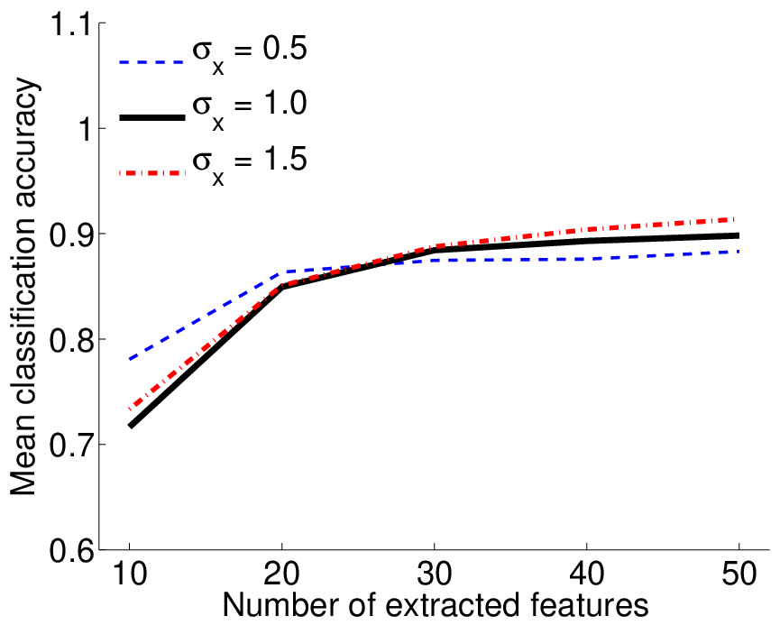
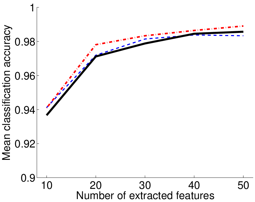
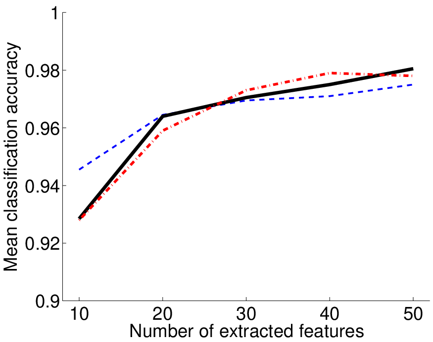
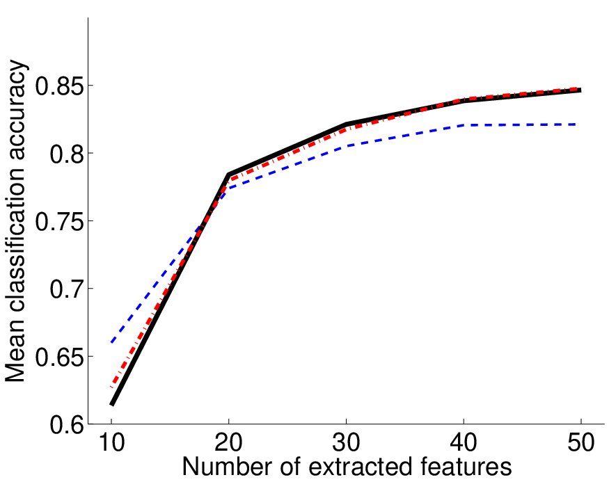
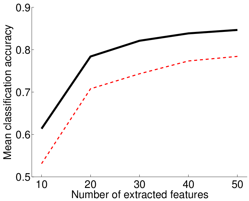
Role of the Gaussian Width and the Output Kernel: In the proposed methods, the Gaussian width and the output kernel must be chosen manually. We carried out a set of experiments to show the sensitivity of choosing the Gaussian width and the output kernel in Figures 3 and 4. Note that, since the performance of HSIC Lasso and NOCCO Lasso are comparable, we here only evaluate HSIC Lasso. As can be seen in Figure 3, the proposed method is not so sensitive to the Gaussian width. From the output kernel comparison in Figure 4, we found that HSIC Lasso with delta kernel clearly outperforms that with Gaussian kernel. Thus using different input and output kernels is important for feature selection in classification scenarios.
4.3.2 High-Dimensional Regression
We also evaluate our proposed method with the Affymetric GeneChip Rat Genome 230 2.0 Array data set (Scheetz et al., 2006). The data set consists of 120 rat subjects with 31098 genes which were measured from eye tissue. Similar to Huang et al. (2010), we focus on finding genes that are related to the TRIM32 gene, which was recently found to cause the Bardet-Biedl syndrome. Note that, since TRIM32 takes real values, this is a regression problem.
In this experiment, we use 80 of samples for training and the rest for testing. We repeat the experiments 100 times by randomly shuffling training and test samples, and evaluate the performance of feature selection methods by the mean squared error. In addition, we use the correlation coefficient between the predicted and the true TRIM32 values, which is a popular performance metric in biology community. We use kernel regression (KR) (Schölkopf and Smola, 2002) with the Gaussian kernel for evaluating the mean squared error and the mean correlation when the top features selected by each method are used. We first choose 50 features and then use top features having the largest absolute regression coefficients. In KR, all tuning parameters such as the Gaussian width and the regularization parameter are chosen based on 3-fold cross-validation.
Results: Figure 5 shows the mean squared error and the mean correlation coefficient over 100 runs as functions of the number of selected features. As can be observed, the proposed HSIC Lasso and NOCCO Lasso compare favorably with existing methods.

(a) MSE

(b) MSE (HSIC Lasso)

(c) MSE (NOCCO Lasso)

(d) Mean correlation coefficient

(e) Mean correlation coefficient (HSIC Lasso)

(f) Mean correlation coefficient (NOCCO Lasso)
5 Conclusion
In this paper, we proposed novel non-linear feature selection methods called HSIC Lasso and NOCCO Lasso. In the proposed methods, global optimal solutions can be obtained by solving a Lasso optimization problem with a non-negativity constraint, which can be efficiently performed by the dual augmented Lagrangian algorithm (Tomioka et al., 2011). Furthermore, the proposed methods have clear statistical interpretation that non-redundant features with strong statistical dependence on output values can be found via kernel-based independence measures (Gretton et al., 2005; Fukumizu et al., 2008). We applied the proposed methods to real-world image and biological feature selection tasks, and experimentally showed that they are promising.
The usefulness of the proposed method will be further investigated on more real-world applications such as computer vision, bioinformatics, and speech and signal processing in the future work. Moreover, extending the proposed model to multi-task learning and prediction and investigating theoretical properties of the proposed formulation are important issues to be investigated.
Acknowledgments
The authors thank Prof. Pradeep Ravikumar for providing us the SpAM code and Dr. Junming Yin and Dr. Kenji Fukumizu for their valuable comments. MY acknowledges the JST PRESTO Program and the PLIP Program, WJ acknowledges the Okazaki Kaheita International Scholarship and MEXT KAKENHI 23120004, and MS acknowledges the FIRST program.
References
- Bach (2008) Bach, F. (2008). Bolasso: Model consistent lasso estimation through the bootstrap. In International Conference on Machine learning (ICML), pages 33–40. ACM.
- Bach (2009) Bach, F. (2009). Exploring large feature spaces with hierarchical multiple kernel learning. In Advances in Neural Information Processing Systems (NIPS), pages 105–112.
- Boyd and Vandenberghe (2004) Boyd, S. and Vandenberghe, L. (2004). Convex Optimization. Cambridge University Press, Cambridge.
- Combettes and Wajs (2005) Combettes, P. L. and Wajs, V. R. (2005). Signal recovery by proximal forward-backward splitting. Multiscale Modeling and Simulation, 4(4), 1168–1200.
- Cortes et al. (2012) Cortes, C., Mohri, M., and Rostamizadeh, A. (2012). Algorithms for learning kernels based on centered alignment. Journal of Machine Learning Research (JMLR), 13, 795–828.
- Cover and Thomas (2006) Cover, T. M. and Thomas, J. A. (2006). Elements of Information Theory. John Wiley & Sons, Inc., Hoboken, NJ, USA, 2nd edition.
- Daubechies et al. (2004) Daubechies, I., Defrise, M., and De Mol, C. (2004). An iterative thresholding algorithm for linear inverse problems with a sparsity constraint. Communications on Pure and Applied Mathematics, LVII(11), 1413–1457.
- Ding and Peng (2005) Ding, C. and Peng, H. (2005). Minimum redundancy feature selection from microarray gene expression data. Journal of Bioinformatics an Computaitonal Biology, 3(2), 185–205.
- Forman (2008) Forman, G. (2008). Bns feature scaling: An improved representation over tf-idf for svm text classification. In ACM Conference on Information and Knowledge Management (CIKM), pages 263–270.
- Fukumizu et al. (2008) Fukumizu, K., Gretton, A., Sun, X., and Schölkopf, B. (2008). Kernel measures of conditional dependence. In J. Platt, D. Koller, Y. Singer, and S. Roweis, editors, Advances in Neural Information Processing Systems, pages 489–496, Cambridge, MA. MIT Press.
- Gretton et al. (2005) Gretton, A., Bousquet, O., Smola, A., and Schölkopf, B. (2005). Measuring statistical dependence with Hilbert-Schmidt norms. In Algorithmic Learning Theory (ALT), pages 63–77. Springer.
- Hastie et al. (2001) Hastie, T., Tibshirani, R., and Friedman, J. (2001). The Elements of Statistical Learning: Data Mining, Inference, and Prediction. Springer, New York.
- Huang et al. (2010) Huang, J., Horowitz, J. L., and Wei, F. (2010). Variable selection in nonparametric additive models. Annals of statistics, 38(4), 2282.
- Kim et al. (2007) Kim, S.-J., Koh, K., Lustig, M., Boyd, S., and Gorinvesky, D. (2007). An interior-point method for large-scale -regularized least squares. IEEE Journal of Selected Topics in Signal Processing, 1(4), 606–617.
- Li et al. (2006) Li, F., Yang, Y., and Xing, E. (2006). From lasso regression to feature vector machine. In Advances in Neural Information Processing Systems (NIPS), pages 779–786.
- Liu et al. (2009) Liu, H., Lafferty, J., and Wasserman, L. (2009). Nonparametric regression and classification with joint sparsity constraints. In Advances in Neural Information Processing Systems (NIPS), pages 969–976.
- Masaeli et al. (2010) Masaeli, M., Fung, G., and Dy, J. G. (2010). From transformation-based dimensionality reduction to feature selection. In International conference on Machine learning (ICML), pages 751–758.
- Meier et al. (2008) Meier, L., Van De Geer, S., and Bühlmann, P. (2008). The group lasso for logistic regression. Journal of the Royal Statistical Society: Series B (Statistical Methodology), 70(1), 53–71.
- Meinshausen and Bühlmann (2010) Meinshausen, N. and Bühlmann, P. (2010). Stability selection. Journal of the Royal Statistical Society: Series B (Statistical Methodology), 72(4), 417–473.
- Nocedal and Wright (2003) Nocedal, J. and Wright, S. (2003). Numerical Optimization (2nd ed.). Springer-Verlag, Berlin, New York.
- Pearson (1920) Pearson, K. (1920). Notes on the history of correlation. Biometrika, 13(1), 25–45.
- Peng et al. (2005) Peng, H., Long, F., and Ding, C. (2005). Feature selection based on mutual information: Criteria of max-dependency, max-relevance, and min-redundancy. IEEE Transactions on Pattern Analysis and Machine Intelligence (PAMI), 27, 1226–1237.
- Raskutti et al. (2012) Raskutti, G., Wainwright, M., and Yu, B. (2012). Minimax-optimal rates for sparse additive models over kernel classes via convex programming. Journal of Machine Learning Research (JMLR), 13, 389–427.
- Ravikumar et al. (2009) Ravikumar, P., Lafferty, J., Liu, H., and Wasserman, L. (2009). Sparse additive models. Journal of the Royal Statistical Society: Series B (Statistical Methodology), 71(5), 1009–1030.
- Rodriguez-Lujan et al. (2010) Rodriguez-Lujan, I., Huerta, R., Elkan, C., and Cruz, C. S. (2010). Quadratic programming feature selection. Journal of Machine Learning Research (JMLR), 11, 1491–1516.
- Roth (2004) Roth, V. (2004). The generalized Lasso. IEEE Transactions on Neural Networks, 15(1), 16–28.
- Scheetz et al. (2006) Scheetz, T. E., Kim, K.-Y. A., Swiderski, R. E., Philp, A. R., Braun, T. A., Knudtson, K. L., Dorrance, A. M., DiBona, G. F., Huang, J., Casavant, T. L., et al. (2006). Regulation of gene expression in the mammalian eye and its relevance to eye disease. Proceedings of the National Academy of Sciences, 103(39), 14429–14434.
- Schölkopf and Smola (2002) Schölkopf, B. and Smola, A. J. (2002). Learning with Kernels. MIT Press, Cambridge, MA.
- Seeger (2002) Seeger, M. (2002). Covariance kernels from Bayesian generative models. In Advances in Neural Information Processing Systems (NIPS), pages 905–912.
- Shawe-Taylor and Kandola (2002) Shawe-Taylor, N. and Kandola, A. (2002). On kernel target alignment. In Advances in Neural Information Processing Systems (NIPS), pages 367–373.
- Shenoy et al. (2008) Shenoy, P., Miller, K. J., Crawford, B., and Rao, R. N. (2008). Online electromyographic control of a robotic prosthesis. IEEE Transactions on Biomedical Engineering, 55(3), 1128–1135.
- Song et al. (2012) Song, L., Smola, A., Gretton, A., Bedo, J., and Borgwardt, K. (2012). Feature selection via dependence maximization. The Journal of Machine Learning Research, 13, 1393–1434.
- Steinwart (2001) Steinwart, I. (2001). On the influence of the kernel on the consistency of support vector machines. Journal of Machine Learning Research (JMLR), 2, 67–93.
- Suzuki and Sugiyama (2013) Suzuki, T. and Sugiyama, M. (2013). Fast learning rate of multiple kernel learning: Trade-off between sparsity and smoothness. The Annals of Statistics. to appear.
- Suzuki et al. (2009) Suzuki, T., Sugiyama, M., Kanamori, T., and Sese, J. (2009). Mutual information estimation reveals global associations between stimuli and biological processes. BMC Bioinformatics, 10(S52).
- Tibshirani (1996) Tibshirani, R. (1996). Regression shrinkage and selection via the lasso. Journal of the Royal Statistical Society, Series B, 58(1), 267–288.
- Tomioka et al. (2011) Tomioka, R., Suzuki, T., and Sugiyama, M. (2011). Super-linear convergence of dual augmented Lagrangian algorithm for sparsity regularized estimation. Journal of Machine Learning Research (JMLR), 12, 1537–1586.
- Wright et al. (2009) Wright, S. J., Nowak, R. D., and Figueiredo, M. A. T. (2009). Sparse reconstruction by separable approximation. IEEE Transactions on Signal Processing, 57(7).
- Xing et al. (2001) Xing, E. P., Jordan, M. I., Karp, R. M., et al. (2001). Feature selection for high-dimensional genomic microarray data. In International Conference on Machine Learning (ICML), pages 601–608.
- Yamada et al. (2010) Yamada, M., Sugiyama, M., and Matsui, T. (2010). Semi-supervised speaker identification under covariate shift. Signal Processing, 90(8), 2353–2361.
- Yin et al. (2008) Yin, W., Osher, S., Goldfarb, D., and Darbon, J. (2008). Bregman iterative algorithms for L1-minimization with applications to compressed sensing. SIAM Journal of Imaging Sciences, 1(1), 143–168.
- Zhao et al. (2010) Zhao, Z., Wang, L., and Li, H. (2010). Efficient spectral feature selection with minimum redundancy. In AAAI Conference on Artificial Intelligence (AAAI), pages 673–678.
- Zou and Hastie (2005) Zou, H. and Hastie, T. (2005). Regularization and variable selection via the elastic net. Journal of the Royal Statistical Society: Series B (Statistical Methodology), 67(2), 301–320.