Riemann-Roch theory on finite sets

Baker and Norine showed in [1] that a Riemann-Roch formula holds for an analogue of linear systems defined on the vertices of finite connected graphs. There, the image of the graph Laplacian induces a equivalence relation on the group of divisors of the graph, which are integer-valued functions defined on the set of vertices. This equivalence relation is the analogue of linear equivalence in the classical algebro-geometric setting.

We showed in [2] that the Baker-Norine result implies a generalization of the Riemann-Roch formula to edge-weighted graphs, where the edge weights can be $R$-valued, where $R$ is an arbitrary subring of the reals; the equivalence relation induced by image of the edge-weighted graph Laplacian applies equally well to divisors which are $R$-valued functions defined on the set of vertices. In [3], we proved our version of the $R$-valued Riemann-Roch theorem from first principles; this gave an independent proof of the Bake-Norine result as well.

The notion of linear equivalence above is induced by the appropriate graph Laplacian acting on the group of divisors, which may be viewed as points in $\mathbb{Z}^{n}$ (the Baker-Norine case) or more generally $R^{n}$, where $n$ is the number of vertices of the graph. In this paper, we propose a generalization of this Riemann-Roch formula for graphs where linear equivalence is induced by a group action on the points of $R^{n}$. The setup we will use is as follows.

Choose a subring $R$ of the reals, and fix a positive integer $n$. Let $V$ be the group of points in $R^{n}$ under component-wise addition. If $x\in V$, we we will use the functional notation $x(i)$ to denote the the $i$-th component of $x$.

For any $x\in V$, define the degree of $x$ as

For any $d\in R$, define the subset $V_{d}\subset V$ to be

Note that the subset $V_{0}$ is a subgroup; for any $d$, $V_{d}$ is a coset of $V_{0}$ in $V$.

Let $H\subset V_{0}$ be a subgroup of $V_{0}$ and consider the action on $V$ by $H$ by translation: if $h\in H$ and $x\in V$, then $(h,x)\mapsto h+x$. This action of $H$ on $V$ induces the equivalence relation $x\sim y$ if and only if $x-y\in H$; or equivalently, $x\sim y$ if and only if there is a $h\in H$ such that $x=(h,y)$.

Fix the parameter $g\in R$, which we call the genus, and choose a set $\mathcal{N}\subset V_{g-1}$. For $x\in V$, define

where $\max$ and $\min$ are evaluated at each coordinate. It follows that $x=x^{+}+x^{-}$ and $x^{+}=-(-x)^{-}$. We then define the dimension of $x\in V$ to be

We will discuss the motivation for this definition of dimension in the next section.

We can now state our main result.

We will give a proof of Theorem 1.1 in §2. In §3, we will give examples of $H$, $\kappa$, and $\mathcal{N}$ (coming from the graph setting) which satisfy the conditions of Theorem 1.1, and show how this Riemann-Roch formulation is equivalent to that given in [3]. Finally in §4, we gives examples that do not arise from graphs.

The dimension of $x\in V$

can be written as

If $x(i)\geq\nu(i)$ for each $i$, $\sum_{i=1}^{n}\max\{x(i)-\nu(i),0\}$ is the taxicab distance from $x$ to $\nu$. Thus, $\ell(x)$ is the taxicab distance from $x$ to the portion of the set $\mathcal{N}$ such that $x\geq\mathcal{N}$, where the inequality is evaluated at each component.

We will now proceed with the proof of the Riemann-Roch formula.

Note that $\kappa\in V$ is the analogue to the canonical divisor in the classical Riemann-Roch formula.

Let $\Gamma$ be a finite, edge-weighted connected simple graph with $n$ vertices. We will assume that $\Gamma$ has no loops. Let $w_{ij}\in R$ with $w_{ij}\geq 0$ be the weight of the edge connecting vertices $v_{i}$ and $v_{j}$. The no loops assumption is also applied to the edge weights so that $w_{ii}=0$ for each $i$. We showed in [3] that such a graph satisfies an equivalent Riemann-Roch formula as in Theorem 1.1.

In this setting, $H=<h_{1},h_{2},\ldots,h_{n-1}>$ where each $h_{i}\in R^{n}$ is defined as

(Here $\deg(v)$ for a vertex $v$ is the sum of the weights of the edges incident to $v$.) Note that $H$ is the edge-weighted Laplacian of $\Gamma$.

As shown in [3], the set $\mathcal{N}\subset V_{g-1}$ is generated by a set $\{\nu_{1},\ldots,\nu_{s}\}$ as follows. Fix a vertex $v_{k}$ and let $(j_{1},\ldots,j_{n})$ be a permutation of $(1,\ldots,n)$ such that $j_{1}=k$. There are then $(n-1)!$ such permutations; for each permutation, we compute a $\nu\in V_{g-1}$ defined by

Each such $\nu$ may not be unique; set $s$ to be the number of unique $\nu$’s and index this set $\{\nu_{1},\ldots,\nu_{s}\}$. We then define the set $\mathcal{N}$ as

The canonical element $\kappa$ is defined by $\kappa(j)=\deg(v_{j})-2$, and the genus $g=1+\sum_{i<j}w_{ij}-n$.

As an example, consider a two vertex graph $\Gamma$ with edge weight $w_{12}=p>0$. Then $g=p-1$ and $H=<(p,-p)>=\mathbb{Z}(p,-p)$. The set $\mathcal{N}\subset V_{g-1}$ is $\mathcal{N}=\{\nu\mid\nu\sim(p-1,-1)\}$ and $\kappa=(p-2,p-2)$. Figure 1 shows the divisors $x\in\mathbb{R}^{2}$ for this graph in the plane. The shaded region, which is bounded by the corner points in the set $\mathcal{N}$, represent points $x$ with $\ell(x)=0$.

We can show directly that $\mathcal{N}$ and $\kappa$ for the two-vertex graph example satisfy the necessary condition for Theorem 1.1 to hold. If $\kappa-x\in\mathcal{N}$, then $\kappa-x=m(p,-p)+(p-1,-1)$ for some $m\in\mathbb{Z}$. Solving for $x$, we have

and thus $x\in\mathcal{N}$. Similarly, if $\nu\in\mathcal{N}$, it easily follows that $\kappa-\nu\in\mathcal{N}$.

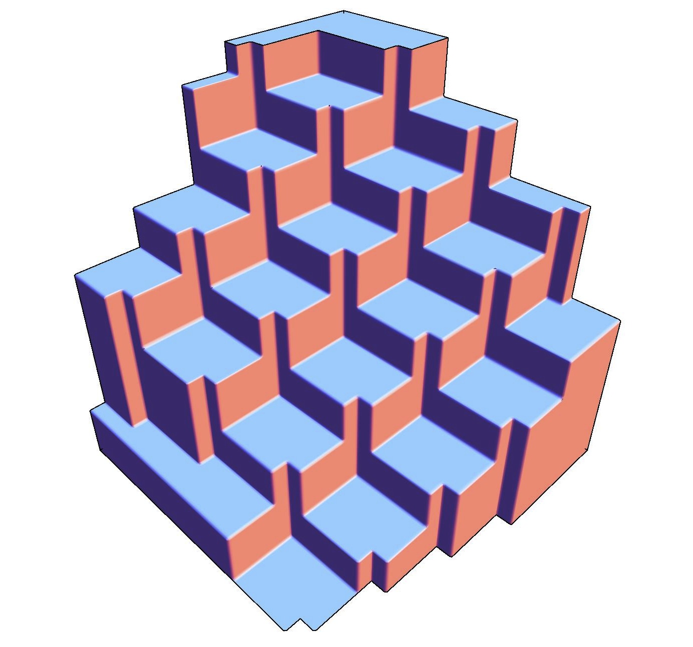
Now consider a three vertex graph with edge weights $w_{12}=p$, $w_{13}=q$ and $w_{23}=r$. The set $\mathcal{N}$ can be generated by $\nu_{1}=(-1,p-1,q+r-1)$ and $\nu_{2}=(-1,p+r-1,q-1)$; $H$ can be generated by $h_{1}=(p+q,-p,-q)$ and $h_{2}=(-p,p+r,-r)$. In Figure 2, the region representing points $x\in\mathbb{R}^{3}$ such that $\ell(x)=0$ is shown for a three vertex graph with edge weights $p=1$, $q=3$ and $r=4$.

The main result of this paper would not be interesting if there were no examples of subgroups $H\subset V_{0}$ with $\mathcal{N}$ and $\kappa$ that were not derived from graphs.

We include in Figure 3 a representation of the divisors $x\in\mathbb{R}^{2}$ with $\ell(x)=0$ for the example used in the proof of Theorem 4.1. The plot is identical to that of a two vertex graph with $p=4$ but is shifted by $-1$ in each direction.

It is also possible to produce non-graph examples by using more generators for $\mathcal{N}$. In Figure 4, the divisors $x\in\mathbb{R}^{2}$ with $\ell(x)=0$ are shown where $\mathcal{N}$ is generated by two points $\nu_{1}=(0,4)$ and $\nu_{2}=(1,3)$, using $H=<(-3,3)>$ and $\kappa=(0,0)$.

References

• [1] Matthew Baker and Serguei Norine, Riemann-Roch and Abel-Jacobi Theory on a Finite Graph, Advances in Mathematics 215 (2007) 766-788.
• [2] Rodney James and Rick Miranda, A Riemann-Roch theorem for edge-weighted graphs, arXiv:0908.1197v2 [math.AG], 2009.
• [3] Rodney James and Rick Miranda, Linear Systems on Edge-Weighted Graphs, arXiv:1105.0227v1 [math.AG], 2011.