Simplified Smooth Inflation with Observable Gravity Waves

^⋆ Department of Physics, University of Basel,

Klingelbergstr. 82, CH-4056 Basel, Switzerland,

^† Bartol Research Institute, Department of Physics and Astronomy,

University of Delaware, Newark, Delaware 19716, USA

Supersymmetric (SUSY) hybrid inflation models [1, 2], provide an interesting possibility of realizing inflation in the grand unified theories (GUTs) of particle physics [3]-[9]. Among its attractive feature are the solution of eta problem, adequately suppressed supergravity (SUGRA) corrections and consistency with the recent WMAP7 data [10]. In the standard version of susy hybrid inflation, gauge symmetry is usually broken at the end of inflation. This implies that the topological defects (such as monopoles), if present, are produced after the inflation and their presence is in contradiction with the experimental observations. In order to solve this problem of topological defects, various extensions of susy hybrid inflation have been proposed. Among all these variants, shifted [5] and smooth [11] hybrid inflation models are the simplest ones. In these models inflation occurs along the ‘shifted’ tracks where gauge symmetry is broken during inflation. This then solves the problem of topological defects by inflating them away and by reducing their density under the observational limits. However, in contrast to shifted hybrid inflation, in the smooth hybrid inflation scenario inflation ends smoothly without any water fall effect.

In this brief report we will consider a simplified version of smooth hybrid inflation model. By simplified we mean that the ultraviolet (UV) cutoff scale of the underlying theory is identified with the reduced Planck mass $m_{P}\simeq 2.4\times 10^{18}$ GeV. As we will show, the potential for smooth hybrid inflation based on a minimal Kähler potential does not realize inflation with sub-Planckian values of the field. However, by employing a non-minimal Kähler potential, one can realize inflation with predictions that are consistent with the WMAP7 data. We obtain in this case a scalar spectral index $n_{s}$ within the WMAP7 1-$\sigma$ bounds, and a large tensor to scalar ratio (canonical measure of gravity waves) $r\lesssim 0.02$. The parameter region explored in this report is expected to be tested soon by the Planck surveyor.

The simplified smooth inflation is defined by the superpotential $W$,

$$W=S\left(\mu^{2}-\frac{(\Phi\overline{\Phi})^{2}}{m_{P}^{2}}\right)\,,$$

(1)

where $S$ is a gauge singlet superfield, $\Phi$ and $\overline{\Phi}$ are a conjugate pair of superfields transforming as nontrivial representations of some gauge group $G$, and $\mu$ is a superheavy mass. Note that in the expression for $W$ the UV cutoff $m_{P}$ (reduced Planck mass) has replaced the cutoff $M_{*}$ normally employed in smooth hybrid inflation models. Both $W$ and $S$ carry the same $R$-charge, while the combination $\Phi\overline{\Phi}$ is neutral under $U(1)_{R}$. In addition, $W$ respects a $Z_{2}$ symmetry under which $S$ is even and the combination $\Phi\overline{\Phi}$ is odd. Thus, $W$ is the most general superpotential with leading order non-renormalizable term which is consistent with the $R$, $Z_{2}$ and gauge symmetries.

The SUGRA scalar potential is given by

$$V_{F}=\left.e^{K/m_{P}^{2}}\left(K_{ij}^{-1}D_{Z_{i}}WD_{Z^{*}_{j}}W^{*}-3m_{P}^{-2}\left|W\right|^{2}\right)\right|_{Z_{i}=z_{i}},$$

(2)

with $z_{i}\in\{s,\,\phi,\,\overline{\phi},\cdots\}$ being the bosonic components of the superfields $Z_{i}\in\{S,\,\Phi,\,\overline{\Phi},\cdots\}$, and we have defined

$\displaystyle D_{Z_{i}}W$

$\displaystyle\equiv$

$\displaystyle\frac{\partial W}{\partial Z_{i}}+m_{P}^{-2}\frac{\partial K}{\partial Z_{i}}W,\,\,\,\,\,\,K_{ij}\equiv\frac{\partial^{2}K}{\partial Z_{i}\partial Z_{j}^{*}},$

$D_{Z_{i}^{*}}W^{*}=\left(D_{Z_{i}}W\right)^{*}$. The minimal Kähler potential can be expanded as

$$K=|S|^{2}+|\Phi|^{2}+|\overline{\Phi}|^{2}.$$

(3)

In the D-flat direction ($\overline{\phi}^{*}=\phi$), and using Eqs. (1, 3) in Eq. (2), we obtain

$$V=\mu^{4}\left[\left(1-\frac{|\phi|^{4}}{M^{4}}\right)^{2}+8\,\frac{|s|^{2}\,|\phi|^{6}}{M^{8}}+\cdots\right],$$

(4)

where $M=\sqrt{\mu\,m_{P}}$ is the vacuum expectation value (vev) of $\phi$ at the global SUSY minimum ($s=0$, $\langle\phi\rangle=M$). This potential is displayed in Fig. 1 which shows two valleys of minima $y_{\pm}(x)$ given in the large $x$ limit by

$$y_{\pm}\equiv\pm\sqrt{\sqrt{1+(3\,x^{2})^{2}}-3\,x^{2}}\approx\pm\frac{1}{\sqrt{6}\,x},$$

(5)

where $y\equiv|\phi|/M$ and $x\equiv|s|/M$.

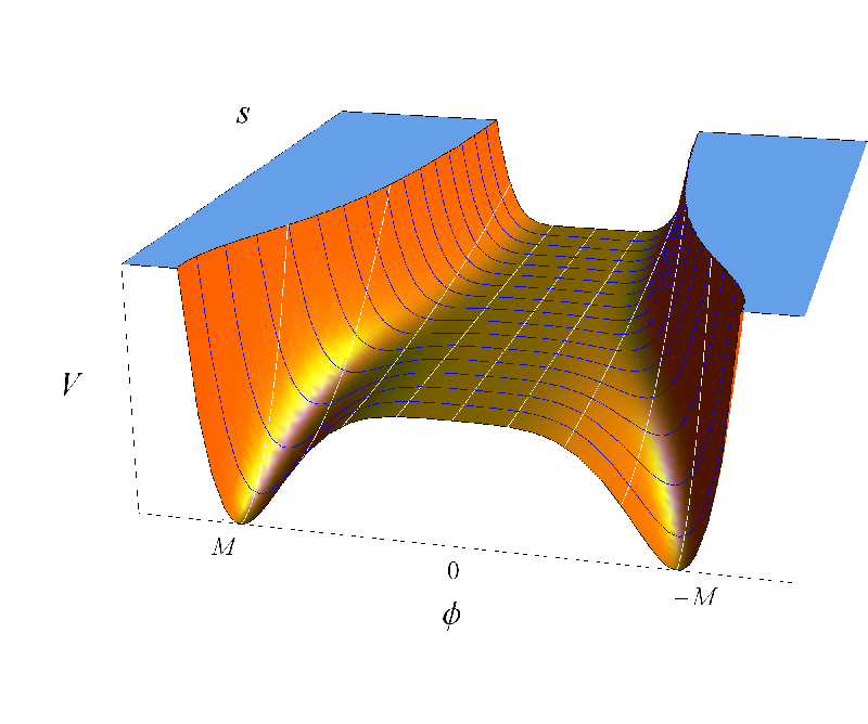
During inflation ($y=y_{+}$ and $x\gg 1$), and excluding SUGRA corrections, the potential is given by,

$$V\simeq\mu^{4}\left(1-\frac{1}{54\,x^{4}}\right).$$

(6)

Using (leading order) slow-roll approximation, the scalar spectral index $n_{s}$, the tensor to scalar ratio $r$, and the running of the scalar spectral index $dn_{s}/d\ln k$ are given by

	$\displaystyle n_{s}$	$\displaystyle\simeq$	$\displaystyle 1+2\,\eta-6\,\epsilon\simeq 1-\frac{5}{3\,N_{0}}$		(7)
	$\displaystyle r$	$\displaystyle\simeq$	$\displaystyle 16\,\epsilon\simeq\frac{8(2\pi\Delta_{\mathcal{R}})^{2/5}}{27N_{0}^{2}}$		(8)
	$\displaystyle\frac{dn_{s}}{d\ln k}$	$\displaystyle\simeq$	$\displaystyle 16\,\epsilon\,\eta-24\,\epsilon^{2}-2\,\xi^{2}\simeq-\frac{5}{3\,N_{0}^{2}}.$		(9)

Here,

$$\epsilon=\frac{1}{4}\left(\frac{m_{P}}{M}\right)^{2}\left(\frac{V^{\prime}}{V}\right)^{2},\,\,\,\eta=\frac{1}{2}\left(\frac{m_{P}}{M}\right)^{2}\left(\frac{V^{\prime\prime}}{V}\right),\xi^{2}=\frac{1}{4}\left(\frac{m_{P}}{M}\right)^{4}\left(\frac{V^{\prime}V^{\prime\prime\prime}}{V^{2}}\right),\,\,\,$$

(10)

$N_{0}$ is the number of e-folds during inflation,

$$N_{0}=2\left(\frac{M}{m_{P}}\right)^{2}\int_{x_{e}}^{x_{0}}\left(\frac{V}{V^{\prime}}\right)dx,$$

(11)

and the amplitude of the curvature perturbation is given by

$$\Delta_{\mathcal{R}}^{2}=\frac{1}{24\,\pi^{2}}\left.\left(\frac{V/m_{P}^{4}}{\epsilon}\right)\right|_{x=x_{0}},$$

(12)

where $\Delta_{\mathcal{R}}^{2}=(2.43\pm 0.11)\times 10^{-9}$ is the WMAP7 normalization at $k_{0}=0.002\,\rm{Mpc}^{-1}$ [10]. The quantity $x_{0}$ denotes the field value at the pivot scale $k_{0}$, and $x_{e}$ is the field value at the end of inflation, defined by $|\eta(x_{e})|=1$. For $N_{0}=50$, we obtain $n_{s}\simeq 0.968$, $r\simeq 3\times 10^{-6}$ and $dn_{s}/d\ln k\simeq-7\times 10^{-4}$, with $x_{0}\simeq 5$ and $M\simeq 6\times 10^{16}$ GeV.

Including SUGRA corrections [12] with minimal (canonical) Kähler potential modifies the above potential,

$$V_{\mathrm{SUGRA}}\simeq\mu^{4}\left(1-\frac{1}{54\,x^{4}}+\left(\frac{M}{m_{P}}\right)^{2}\frac{8}{54\,x^{2}}+\left(\frac{M}{m_{P}}\right)^{4}\frac{x^{4}}{2}\right).$$

(13)

Taking values of $x_{0}$ and $M$ extracted from the global susy potential one easily checks that the sugra corrections dominate the global susy part. Thus, sugra corrections can be expected to significantly alter the predictions of $n_{s}$ and $r$ found earlier. In ‘simplified smooth hybrid inflation’ ($M_{*}=m_{P}$) with minimal (canonical) Kähler potential, these sugra corrections require transplanckian field values corresponding to $50$-$60$ e-folds of inflation. However, this requirement invalidates the sugra expansion itself. This is in contrast to ‘standard smooth hybrid inflation’ where the cutoff scale $M_{*}$ is allowed to vary below $m_{P}$. Thus by suppressing sugra corrections somewhat we can obtain values of $n_{s}$ just inside the WMAP7 2-$\sigma$ bounds, although with tiny values of $r$.

In order to obtain WMAP7 consistent red-tilted spectrum ($n_{s}\simeq 0.97$) with observable values of $r$ in the simplified smooth hybrid inflation, we consider, following Refs. [15, 16], a non-minimal Kähler potential. [For ‘regular and standard smooth hybrid inflation’ with non-minimal Kähler potential see Refs. [17, 18]]. The Kähler potential with non-minimal terms is given by,

	$\displaystyle K$	$\displaystyle=$	$\displaystyle|S|^{2}+|\Phi|^{2}+|\overline{\Phi}|^{2}$		(14)
			$\displaystyle+\kappa_{S}\frac{|S|^{4}}{4\,m_{P}^{2}}+\kappa_{\Phi}\frac{|\Phi|^{4}}{4\,m_{P}^{2}}+\kappa_{\overline{\Phi}}\frac{|\overline{\Phi}|^{4}}{4\,m_{P}^{2}}+\kappa_{S\Phi}\frac{|S|^{2}|\Phi|^{2}}{m_{P}^{2}}+\kappa_{S\overline{\Phi}}\frac{|S|^{2}|\overline{\Phi}|^{2}}{m_{P}^{2}}+\kappa_{\Phi\overline{\Phi}}\frac{|\Phi|^{2}|\overline{\Phi}|^{2}}{m_{P}^{2}}$
			$\displaystyle+\kappa_{SS}\frac{|S|^{6}}{6\,m_{P}^{4}}+\cdots\,.$

The corresponding scalar potential takes the following form,

$$V\simeq\mu^{4}\left(1-\frac{1}{54\,x^{4}}+\left(-\kappa_{S}\,x^{2}+\frac{8+3\,\kappa_{S}}{54\,x^{2}}\right)\left(\frac{M}{m_{P}}\right)^{2}+\gamma_{S}\left(\frac{M}{m_{P}}\right)^{4}\frac{x^{4}}{2}\right),$$

(15)

where $\gamma_{S}=1-\frac{7\kappa_{S}}{2}+2\kappa_{S}^{2}-3\kappa_{SS}$. We have suppressed radiative corrections in the above potential since there is no direct renormalizable coupling of the inflaton with the other fields. We have also ignored the soft susy breaking terms as their contribution will be negligible in the parameter range consistent with the WMAP7 (2$\sigma$) bounds [13, 14].

The predictions for the various inflationary parameters are obtained by employing the slow-roll approximation and are displayed in Figs. (2-4). To achieve better precision in the numerical results, we have also included the next-to-leading order corrections [19, 20] in the slow roll expansion for the quantities $n_{s}$, $r$, $dn_{s}/d\ln k$, and $\Delta_{\mathcal{R}}$. We require $(|\kappa_{S}|,\,|\kappa_{SS}|)\leq 1$ and $|s_{0}|\leq m_{P}$. In Fig. (2) we have presented the behavior of $r$ and $\mu$ with respect to $n_{s}$ along with the WMAP7 1-$\sigma$ and 2-$\sigma$ bounds. The upper bound on $r$ comes from the constraint $|s_{0}|\leq m_{P}$, whereas the lower boundary curve represents the $\kappa_{SS}=-1$ constraint. These plots show that with the help of non-minimal Kähler potential, $r$ can be increased by up to four orders of magnitudes as compared to its value from the global susy potential. The large $r$ solutions, however, require values of $M$ larger than the grand unified theory (GUT) scale $\sim 2\times 10^{16}$ (see Fig. (3)). From Eq. (12) and the definition $M\equiv\sqrt{\mu\,m_{P}}$, one finds the following approximate relation,

$$r\simeq\left(\frac{2}{3\,\pi^{2}\,\Delta_{\mathcal{R}}^{2}}\right)\left(\frac{M}{m_{P}}\right)^{8}=\left(\frac{M}{3.35\times 10^{16}\,GeV}\right)^{4}\left(\frac{M}{m_{P}}\right)^{4}.$$

(16)

This relation provides a reasonable estimate of the otherwise more accurately calculated numerical result displayed in Fig. (3). However, this relation alone is insufficient to explain the upper bound on the values of $r$ which is discussed below in some detail. Furthermore, the values of $dn_{s}/d\ln k$ shown in the right panel of Fig. (3) are reasonably small and in accord with the WMAP7 data assumptions.

In Fig. (4), left panel, we show how $r$ varies with respect to $\kappa_{S}$, while the right panel shows the relationship between $\kappa_{SS}$ and $\gamma_{S}$ to $\kappa_{S}$. As anticipated, the minimal case with $(\kappa_{S},\,\kappa_{SS})=(0,0)$ is not consistent with the WMAP7 1-$\sigma$ and 2-$\sigma$ bounds. Moreover, in agreement with earlier observations (Refs. [15, 16, 21]), large (observable) $r$ solutions are obtained with the potential form, $V/\mu^{4}\simeq 1+$ quadratic - quartic, with $(\kappa_{S},\,\gamma_{S})<(0,0)$, as shown in the right panel of Fig. (4). This behavior can be explained with the requirements $V^{\prime}(x_{0})>0$ and $V^{\prime\prime}(x_{0})<0$ (or $n_{s}<1$), with $\epsilon(x_{0})\ll\eta(x_{0})$ at the pivot scale. Consider the following approximate form of $\epsilon$ and $\eta$,

$$\epsilon\simeq f^{2}\left(\frac{(M/m_{P})^{4}}{27\,f^{6}}-\kappa_{S}+\gamma_{S}\,f^{2}\right)^{2},\,\,\,\eta\simeq\frac{5\,(M/m_{P})^{4}}{27\,f^{6}}-\kappa_{S}+3\,\gamma_{S}\,f^{2},$$

(17)

where, $f\equiv|s|/m_{P}$. In the large $r$ limit, the contribution from the global susy part of the potential is negligible at the pivot scale, and it becomes important only near the end of inflation. After neglecting this contribution, one can check that the choice $(\kappa_{S},\,\gamma_{S})<(0,0)$ is the only possibility which is consistent with large values of $r$ and a red-tilted spectrum $n_{s}<1$.

Next we turn our attention to the explanation of the upper bound on $r$. It might be tempting to justify the observed upper limit on $r$ through the well known bound [22],

$$r\lesssim 0.006\left(\frac{50}{N_{0}}\right)^{2}\left(\frac{\Delta s}{m_{P}}\right)^{2},$$

(18)

which is derived with the assumption of a monotonically increasing $\epsilon$ during inflation. With $N_{0}=50$ and $s_{0}=m_{P}$, the bound in eq. (18) predicts $r\lesssim 0.006$, which is in apparent contradiction with our result $r\lesssim 0.02$. Actually, the assumption of monotonically increasing $\epsilon$ breaks down for the large $r$ solutions, as shown explicitly in Fig. (5) for the central value of the scalar spectral index $n_{s}=0.968$. (Also, see Refs. [23, 24] for large $r$ solutions with small field excursions in the context of this bound.).

Let us consider the following relation for the variation of $\epsilon$,

$$\epsilon^{\prime}(x)=2\left(\frac{M}{m_{P}}\right)\sqrt{\epsilon}\,(\eta-2\,\epsilon).$$

(19)

During inflation $\eta$ remains dominant over $\epsilon$ and controls the evolution of $\epsilon$. For large $r$ solutions inflation starts and ends with $\eta<0$ (recall that $\eta(x_{0})<0$ is required for red-tilted spectrum and $\eta(x_{e})=-1$), while passing through the inflection point $\eta=0$. The change in the sign of $\eta$ actually introduces the non-monotonic behavior of $\epsilon$ as shown in Fig. (5). Therefore, Eq. (18) underestimates the upper bound on $r$ in this case.

It is interesting to note that the small $r$ solutions do exhibit a monotonic behavior of $\epsilon$ (see the right panel of Fig. (5)). This comes from the fact that the small $r$ solutions favor $(\kappa_{S},\,\gamma_{S})>(0,0)$, since large values of the field generate a blue-tilted spectrum $n_{s}>1$ caused by positive values of $\eta(x_{0})>\epsilon(x_{0})>0$. Therefore, during inflation the quartic term remains sub-dominant and this makes $\eta$ negative and $\epsilon$ monotonically increasing.

In order to provide a semi-analytical estimate for the upper bound on $r$, we employ Eqs. (16-17) with $f_{0}=1$ to approximate the number of e-folds,

$$N_{0}\simeq\frac{1}{-6\,\kappa_{S}}\ln\left[\frac{27}{20}\left(\frac{m_{P}}{3.35\times 10^{16}\,GeV}\right)^{2}\frac{-\,\kappa_{S}^{3}}{\left(-\kappa_{S}+\gamma_{S}\right)^{4}}\right],$$

(20)

with,

$$\gamma_{S}\simeq-\left(\frac{1-n_{s}-4\,\kappa_{S}}{6}\right),\,\,\,r\simeq 16\,(-\kappa_{S}+\gamma_{S})^{2}.$$

(21)

Now, for a given value of $n_{s}$ and $N_{0}$, one can calculate the values of $\kappa_{S}$, $\gamma_{S}$ and $r$. For $n_{s}=0.968$ we obtain $\kappa_{S}\simeq-0.047$, $\gamma_{S}\simeq-0.026$ and $r\simeq 0.011$, which is in good agreement with our numerical results.

To summarize, we have considered a simplified version of smooth hybrid inflation with a single UV cutoff $m_{P}$. With minimal Kähler potential, the presence of sugra corrections invalidates the otherwise successful inflation obtained with the global susy part of the potential. However, with a non-minimal extension of the Kähler potential we obtain a red-tilted spectrum consistent with the WMAP7 data, and we also achieve up to four orders of magnitude increase in the value of $r(\sim 0.02)$, compared to the global susy result $r\sim 10^{-6}$. These large $r$ solutions can be expected to be observed by the PLANCK satellite.

References

- [1] G. R. Dvali, Q. Shafi and R. K. Schaefer, Phys. Rev. Lett. 73, 1886 (1994) [arXiv:hep-ph/9406319].
- [2] E. J. Copeland, A. R. Liddle, D. H. Lyth, E. D. Stewart and D. Wands, Phys. Rev. D 49, 6410 (1994) [arXiv:astro-ph/9401011].
- [3] V. N. Senoguz and Q. Shafi, Phys. Lett. B 567, 79 (2003) [hep-ph/0305089].
- [4] L. Covi, G. Mangano, A. Masiero and G. Miele, Nucl. Phys. Proc. Suppl. 70, 126 (1999); B. Kyae and Q. Shafi, Phys. Lett. B 597, 321 (2004) [hep-ph/0404168]; S. Khalil, M. U. Rehman, Q. Shafi and E. A. Zaakouk, Phys. Rev. D 83, 063522 (2011) [arXiv:1010.3657 [hep-ph]].
- [5] R. Jeannerot, S. Khalil, G. Lazarides and Q. Shafi, JHEP 0010, 012 (2000) [arXiv:hep-ph/0002151].
- [6] B. Kyae and Q. Shafi, Phys. Rev. D 72, 063515 (2005) [hep-ph/0504044].
- [7] G. Lazarides, I. N. R. Peddie and A. Vamvasakis, Phys. Rev. D 78, 043518 (2008) [arXiv:0804.3661 [hep-ph]].
- [8] B. Kyae and Q. Shafi, Phys. Lett. B 635, 247 (2006) [hep-ph/0510105]; M. U. Rehman, Q. Shafi and J. R. Wickman, Phys. Lett. B 688, 75 (2010) [arXiv:0912.4737 [hep-ph]].
- [9] S. Antusch, M. Bastero-Gil, J. P. Baumann, K. Dutta, S. F. King and P. M. Kostka, JHEP 1008, 100 (2010) [arXiv:1003.3233 [hep-ph]].
- [10] E. Komatsu et al. [WMAP Collaboration], Astrophys. J. Suppl. 192, 18 (2011) [arXiv:1001.4538 [astro-ph.CO]].
- [11] G. Lazarides and C. Panagiotakopoulos, Phys. Rev. D 52, R559 (1995) [hep-ph/9506325].
- [12] A. D. Linde and A. Riotto, Phys. Rev. D 56, 1841 (1997) [arXiv:hep-ph/9703209].
- [13] V. N. Senoguz and Q. Shafi, Phys. Rev. D 71, 043514 (2005) [hep-ph/0412102].
- [14] M. U. Rehman, Q. Shafi and J. R. Wickman, Phys. Lett. B 683, 191 (2010) [arXiv:0908.3896 [hep-ph]].
- [15] Q. Shafi and J. R. Wickman, Phys. Lett. B 696, 438 (2011) [arXiv:1009.5340 [hep-ph]]; M. U. Rehman, Q. Shafi and J. R. Wickman, Phys. Rev. D 83, 067304 (2011) [arXiv:1012.0309 [astro-ph.CO]].
- [16] M. Civiletti, M. U. Rehman, Q. Shafi and J. R. Wickman, Phys. Rev. D 84, 103505 (2011) [arXiv:1104.4143 [astro-ph.CO]].
- [17] M. Bastero-Gil, S. F. King and Q. Shafi, Phys. Lett. B 651, 345 (2007) [hep-ph/0604198].
- [18] M. ur Rehman, V. N. Senoguz and Q. Shafi, Phys. Rev. D 75, 043522 (2007) [hep-ph/0612023].
- [19] E. D. Stewart and D. H. Lyth, Phys. Lett. B 302, 171 (1993) [arXiv:gr-qc/9302019].
- [20] V. N. Senoguz and Q. Shafi, Phys. Lett. B 668, 6 (2008) [arXiv:0806.2798 [hep-ph]].
- [21] M. U. Rehman, Q. Shafi and J. R. Wickman, Phys. Rev. D 79, 103503 (2009) [arXiv:0901.4345 [hep-ph]].
- [22] D. H. Lyth, Phys. Rev. Lett. 78, 1861 (1997) [hep-ph/9606387].
- [23] I. Ben-Dayan and R. Brustein, JCAP 1009, 007 (2010) [arXiv:0907.2384 [astro-ph.CO]].
- [24] S. Hotchkiss, A. Mazumdar and S. Nadathur, arXiv:1110.5389 [astro-ph.CO].