High order asymptotic-preserving schemes for the Boltzmann equation

Giacomo Dimarco ^†^†thanks: Université de Toulouse; UPS, INSA, UT1, UTM; CNRS, UMR 5219; Institut de Mathématiques de Toulouse; F-31062 Toulouse, France. (giacomo.dimarco@math.univ-toulouse.fr). Lorenzo Pareschi ^†^†thanks: Mathematics Department, University of Ferrara and CMCS, Ferrara, Italy (lorenzo.pareschi@unife.it).

Abstract

In this note we discuss the construction of high order asymptotic preserving numerical schemes for the Boltzmann equation. The methods are based on the use of Implicit-Explicit (IMEX) Runge-Kutta methods combined with a penalization technique recently introduced in [6].

Keywords: Implicit-Explicit Runge-Kutta methods, stiff equations, Boltzmann equation, fluid limits, asymptotic preserving schemes.

Schémas d’ordre élévé et préservant l’asymptotique pour l’équation de Boltzmann

Résumé

Dans cette note nous discutons la construction de schémas d’ordre élevé pour l’équation de Boltzmann qui préservent la limite asymptotique. Les méthodes sont basées sur l’utilisation de schémas de Runge-Kutta explicites-implicites combinées avec une technique de pénalisation introduit récemment par [6].

Mots-clés : Méthodes Runge-Kutta Implicites-Explicites, équations raides, équation de Boltzmann, limite fluide, schémas préservant l’asymptotique.

Version française abrégée

Les équations cinétiques, comme l’équation de Boltzmann sont utilisé avec succès dans de nombreuses applications réelles. L’équation de Boltzmann décrit l’évolution temporelle de la fonction de distribution d’un gaz avec des interactions binaires élastiques. Il est importante de mentionner que la solution numérique de l’opérateur de collision représente un défi majeur pour les méthodes numériques traditionnelles qui n’est pas encore résolu. Cela est particulièrement vrai en proximité des régimes fluides. Dans ces régimes le taux des collisions intermoléculaires croît de façon exponentielle et donc le temps entre deux collisions successives devient très petit. D’autre part, l’échelle de temps réel pour l’évolution du gaz est l’échelle de temps de la dynamique des fluides, qui est normalement beaucoup plus grande que le temps entre deux collisions. Une mesure de l’importance des collisions est donnée par le nombre de Knudsen $\varepsilon$ , qui est grand dans la limite raréfiée et petit dans la limite fluide. Ainsi, les approches numériques traditionnelles perdent leur efficacité en raison de la nécessité d’utiliser de temps très petits pour la discretization temporelle. Nous rappelons que la discrétisation directe en temps de l’équation de Boltzmann est un gros problème dans les régimes raides en raison de la haute dimensionnalité et de la non-linéarité de l’opérateur de collision qui rend peu pratique l’utilisation de solveurs implicites.

Plusieurs auteurs ont abordé le problème dans le récent passé( voir [4, 5, 6, 8, 9, 11]) et les références á l’intérieur). Une stratégie, parmi les plus puissantes, consiste en la construction des schémas dits préservant l’asymptotique. Ces techniques permettent de résoudre le problème dans tout le domaine pour tous les choix de pas de temps et de nombre de Knudsen. Dans cette note, nous proposons une nouvelle classe de schemas Runge-Kutta Implicites-Explicites pour l’équation de Boltzmann. Pour construire nos schemas, nous considérons une décomposition du terme de gain de l’opérateur de collision en un partie en équilibre et en une partie en non équilibre. Cette décomposition de l’intégrale de Boltzmann a été également introduite par Jin et Filbet dans [6]. Les principaux avantages de l’approche proposée ici est que cela fonctionne de manière uniforme pour une large gamme de nombres de Knudsen et évite la solution d’un système d’équations non linéaires, même dans les régimes raides. De même que pour [4], nous obtenons des conditions suffisantes pour la stabilité asymptotique et la préservation asymptotique de l’ordre temporel des schemas. En plus, nous construirons les schémas tels qu’ils préservent la positivité des solutions et les quantités physiques conservées. Pour plus de détails nous renvoyons à [5].

1 Introduction

The computation of fluid-kinetic interfaces and asymptotic behaviors involves multiple scales where most numerical methods lose their efficiency because they are forced to operate on a very short time scale (see [4, 5, 6, 8, 9, 11] and the references therein for a more complete bibliography). The Boltzmann equation close to fluid regimes represents the prototype example

\partial_{t}f+v\cdot\nabla_{x}f=\frac{1}{\varepsilon}Q(f,f).

(1)

Here $f(x,v,t)$ is a non negative function describing the time evolution of the distribution of particles with velocity $v\in\R^{3}$ and position $x\in\Omega\subset\R^{d_{x}}$ at time $t>0$ .

The operator $Q(f,f)$ describes the particles interactions. In the general case of the Boltzmann binary collision, it has the form

Q_{B}(f,f)=\int_{\mathbb{R}^{3}\times S^{2}}B(|v-v_{*}|,n)[f(v^{\prime})f(v^{\prime}_{*})-f(v)f(v_{*})]\,dv_{*}\,dn

(2)

where

v^{\prime}=v+\frac{1}{2}(v-v_{*})+\frac{1}{2}|v-v_{*}|n,\quad v^{\prime}_{*}=v+\frac{1}{2}(v-v_{*})-\frac{1}{2}|v-v_{*}|n,

(3)

and $B(|v-v_{*}|,n)$ is a nonnegative collision kernel characterizing the details of the collision.

The Knudsen number $\varepsilon>0$ is a non dimensional measure of the importance of collisions and is large in rarefied regions and small where the system is close to the fluid limit. In the latter regime, the intermolecular collision rate grows quickly and thus the collisional time scale becomes very small. On the other hand, the actual time scale of the evolution is the fluid dynamic scale, which can be much larger than the collisional time.

In fact, for small values of $\varepsilon$ the distribution function is well approximated by a local Maxwellian

M[f]=\frac{\rho}{(2\pi T)^{3/2}}\exp\left(\frac{-|w-v|^{2}}{2T}\right),

(4)

where $\rho$ , $w$ , $T$ are the density, mean velocity and temperature of the gas in the x-position and at time $t$ defined as

(\rho,\rho w,E)^{T}=\int_{\mathbb{R}^{3}}f\left(1,v,\frac{v^{2}}{2}\right)^{T}\,dv,\qquad T=\frac{1}{3\rho}(E-\rho|w|^{2}).

(5)

Now, passing to the limit for $\varepsilon\rightarrow 0$ and integrating (1) against $1$ , $v$ and $v^{2}$ we recover the system of compressible Euler equations

\partial_{t}u+\nabla_{x}\cdot F(u)=0

(6)

with

u=(\rho,w,E)^{T},\qquad F(u)=(\rho w,\varrho w\otimes(w+pI),Ew+pw)^{T},\quad p=\rho T,

where $I$ is the identity matrix.

Implicit-Explicit (IMEX) Runge-Kutta schemes represent a powerful tool for the numerical treatment of stiff terms in PDEs [4, 3, 11]. When necessary they can be designed in order to achieve suitable asymptotic preserving (AP) properties. Their direct application to the Boltzmann equation however is not trivial since the complicated nonlinear structure of the collisional operator makes prohibitively expensive the use of implicit solvers for the stiff collision term. Additional difficulties are given by the need to preserve the most relevant physical properties of the solution, like conservation of mass, momentum and energy, nonnegativity and entropy inequality. In this short note we will illustrate how the introduction of a suitable penalization technique as in [6] permits to extend succesfully the IMEX formalism also to the challenging case of the Boltzmann equation.

2 IMEX schemes for the Boltzmann equation

In order to apply efficiently the IMEX Runge-Kutta approach to the Boltzmann equation we must avoid the prohibitive cost of the implicit evaluation of the stiff collision term. In order to achieve this we first reformulate the collision part using a suitable penalization term.

2.1 Decomposition of the collision integral

First, we observe that we can rewrite $Q_{B}(f,f)$ as [7]

Q_{B}(f,f)=\frac{1}{\varepsilon}(P(f,f)-\mu f),

(7)

where $P(f,f)=Q_{B}(f,f)+\mu f$ and $\mu>0$ is a constant such that $P(f,f)\geq 0$ .

Observe that, by construction, the following property is verified by the operator $P(f,f)$

\frac{1}{\mu}\int_{\R^{3}}P(f,f)\left(1,v,\frac{v^{2}}{2}\right)^{T}\,dv=\int_{\R^{3}}f\left(1,v,\frac{v^{2}}{2}\right)^{T}\,dv=u.

(8)

Thus, $P(f,f)/\mu$ is a density function and we can consider the following decomposition

P(f,f)/\mu=M[f]+g,

(9)

where the function $g$ represents the deviations from equilibrium of $P(f,f)$ .

Thus the collision operator can be rewritten in the form

Q_{B}(f,f)=\frac{\mu}{\varepsilon}g+\frac{\mu}{\varepsilon}(M[f]-f)=\frac{\mu}{\varepsilon}\left(\frac{P(f,f)}{\mu}-M[f]\right)+\frac{\mu}{\varepsilon}(M[f]-f).

(10)

The above reformulation is equivalent to the penalization method for the collision operator recently introduced in [6]. Clearly, since the problem is stiff as a whole a fully implicit method should be used in the numerical integration to avoid stability constraints of the type $\Delta t=O(\varepsilon)$ . On the other hand, the linear part itself $(M[f]-f)$ suffices to characterize the correct large time behavior of $f$ . Therefore, instead of fully implicit methods, one may use methods which are implicit in the linear part and explicit in the non-linear part. This however, as we will see, introduces some additional stability requirements in order for the IMEX schemes to preserve the asymptotic behavior of the equation.

2.2 Application to the Boltzmann equation

We can now introduce the general class of IMEX Runge-Kutta schemes for the Boltzmann equation in the form

	$\displaystyle F^{(i)}=\displaystyle f^{n}+\Delta t\sum_{j=1}^{i-1}\widetilde{a}_{ij}\left(\frac{\mu}{\varepsilon}g(F^{(j)})-v\cdot\nabla_{x}F^{(j)}\right)+\Delta t\sum_{j=1}^{i}a_{ij}\frac{\mu}{\varepsilon}(M[F^{(j)}]-F^{(j)})$		(11)
	$\displaystyle f^{n+1}=\displaystyle f^{n}+\Delta t\sum_{i=1}^{\nu}\widetilde{\omega}_{i}\left(\frac{\mu}{\varepsilon}g(F^{(i)})-v\cdot\nabla_{x}F^{(i)}\right)+\Delta t\sum_{i=1}^{\nu}\omega_{i}\frac{\mu}{\varepsilon}(M[F^{(i)}]-F^{(i)}).$		(12)

In the above scheme the explicit method is characterized by the $\nu\times\nu$ matrix $\widetilde{A}=(\widetilde{a}_{ij})$ , $\widetilde{a}_{ij}=0$ , $j\geq i$ and the coefficient vectors are $\widetilde{c}=(\widetilde{c}_{1},\ldots,\widetilde{c}_{\nu})^{T}$ , $\widetilde{c}_{i}=\sum_{j=1}^{i-1}{\widetilde{a}_{ij}}$ , $\widetilde{w}=(\widetilde{w}_{1},\ldots,\widetilde{w}_{\nu})^{T}$ , whereas the implicit method is a diagonally implicit Runge-Kutta (DIRK) defined by the $\nu\times\nu$ matrix $A=(a_{ij})$ , $a_{ij}=0$ , $j>i$ , and the coefficient vectors are $c=(c_{1},\ldots,c_{\nu})^{T}$ , $c_{i}=\sum_{j=1}^{\nu}{a_{ij}}$ , $w=(w_{1},\ldots,w_{\nu})^{T}$ .

Let us first recall the definition of asymptotic preserving property [8]

Definition 1

The IMEX scheme (11-12) for the Boltzmann equation is asymptotic preserving (AP) if in the limit $\epsilon\to 0$ the scheme becomes a consistent discretization of the limit system of the Euler equations (6).

Note that if we multiply the IMEX scheme by the vector of collision invariants $\phi(v)=(1,v,v^{2}/2)^{T}$ and integrate in $v$ we get a moment scheme characterized by the explicit method

	$\displaystyle\displaystyle\int_{\mathbb{R}^{3}}F^{(i)}\phi(v)\,dv=\displaystyle\int_{\mathbb{R}^{3}}f^{n}\phi(v)\,dv-\Delta t\sum_{j=1}^{i-1}\widetilde{a}_{ij}\int_{\mathbb{R}^{3}}v\cdot\nabla_{x}F^{(j)}\phi(v)\,dv$		(13)
	$\displaystyle\displaystyle\int_{\mathbb{R}^{3}}f^{n+1}\phi(v)\,dv=\displaystyle\int_{\mathbb{R}^{3}}f^{n}\phi(v)\,dv-\Delta t\sum_{i=1}^{\nu}\widetilde{\omega}_{i}\int_{\mathbb{R}^{3}}v\cdot\nabla_{x}F^{(i)}\phi(v)\,dv.$		(14)

Thus a sufficient condition for a scheme to satisfy the $AP$ property is that as $\varepsilon\to 0$ we get $F^{(i)}\to M[F^{(i)}]$ , $i=1,\ldots,\nu$ in (11). In addition we must require the kinetic numerical solution $f^{n+1}$ to satisfy some additional numerical stability requirement. We illustrate this aspect in the sequel.

First let us start with the following Lemma [5]

Lemma 1

If all diagonal element of the triangular coefficient matrix $A$ that characterize the DIRK scheme in equations (11-12) are non zero, then

\lim_{\varepsilon\rightarrow 0}F^{(i)}=M[F^{(i)}].

(15)

Formally Lemma 1 guarantees the AP property of the scheme. However, as opposite to the case of hyperbolic systems with relaxation, now because of the decomposition of the collision operator the last level (12) still depends on $\varepsilon$ . After some manipulations it reads

	$\displaystyle f^{n+1}$	$\displaystyle=$	$\displaystyle f^{n}\left(1-\sum_{i,j}{w}_{i}b_{ij}\right)-\Delta t\sum_{i=1}^{\nu}\widetilde{w}_{i}\left(v\cdot\nabla_{x}F^{(i)}-\frac{1}{\varepsilon}g(F^{(i)})\right)$
		$\displaystyle+$	$\displaystyle\Delta t\sum_{i,j,h}{w}_{i}b_{ij}\widetilde{a}_{jh}\left(v\cdot\nabla_{x}F^{(h)}-\frac{1}{\varepsilon}g(F^{(h)})\right)+\sum_{i,j}w_{i}b_{ij}F^{(j)},$

where $b_{ij}$ are the elements of $A^{-1}$ . The above expression turns out to be unbounded as $\varepsilon\to 0$ thus originating an unstable scheme.

We introduce the following definition [2, 5]

Definition 2

An IMEX scheme in the form (11)-(12) is globally stiffly accurate if the following conditions are satisfied

w_{i}=a_{\nu i},\qquad\widetilde{w}_{i}=\widetilde{a}_{\nu i},\quad\forall\,i=1,\ldots,\nu.

(17)

We can finally state the main result [5]

Theorem 1

If $\det A\neq 0$ and the IMEX scheme (11)-(12) is globally stiffly accurate, in the limit $\varepsilon\rightarrow 0$ , the IMEX scheme becomes the explicit RK scheme characterized by ( $\widetilde{A},\widetilde{w},\widetilde{c}$ ) applied to the limit Euler system (6).

In order to prove the Theorem it is enough to observe that the stiffly accurate property implies immediately that $f^{n+1}=F^{(\nu)}$ .

Remark 1

•

Theorem above guarantees not only asymptotic preservation but also asymptotic accuracy, namely the order of the scheme is preserved in the $\varepsilon\to 0$ limit.
•

The previous results can be extended to the case of CK-type schemes [3] with $a_{11}=0$ , like the ones considered in [6]. However in this case asymptotic accuracy holds true only if the initial data are an $O(\varepsilon)$ perturbation of the local Maxwellian equilibrium.

2.3 Convexity of the schemes

The determination of general conditions for positivity of the numerical solution in the space non homogeneous case is quite difficult. Here we focus on the space homogeneous situation. Not that even in this case due to the reformulation of the collision term the analysis involve the whole IMEX scheme. Moreover the analysis here depends on the particular operator used as a penalization.

Using the fact that in the space homogenous situation $M[f]$ does not depend on time the IMEX scheme (11)-(12) can be rewritten as

	$\displaystyle F^{(i)}$	$\displaystyle=$	$\displaystyle\displaystyle\sum_{h=1}^{i}\hat{b}_{ih}\left\{\lambda f^{n}+\sum_{j=1}^{h-1}\widetilde{a}_{hj}\frac{P(F^{(j)},F^{(j)})}{\mu}+\displaystyle M[f^{n}]\left(c_{h}-\widetilde{c}_{h}\right)\right\}$		(18)
	$\displaystyle f^{(n+1)}$	$\displaystyle=$	$\displaystyle\displaystyle f^{n}+\frac{\mu\Delta t}{\varepsilon}\sum_{i=1}^{\nu}\widetilde{w}_{i}\frac{P(F^{(i)},F^{(i)})}{\mu}+\frac{\mu\Delta t}{\varepsilon}\sum_{i=1}^{\nu}w_{i}(M[f^{n}]-F^{(i)})$		(19)

where $\lambda=\varepsilon/(\mu\Delta t)$ and $\hat{b}_{ij}$ are the elements of $(\lambda I+A)^{-1}$ .

The following theorem gives sufficient conditions for the above expression to represent a convex combination of probability densities.

Theorem 2

A sufficient condition to guarantee that $f^{n+1}\geq 0$ when $f^{n}\geq 0$ in (18)-(19) is that the scheme is globally stiffly accurate and the following conditions holds true

0\leq\sum_{h=1}^{i}\hat{b}_{ih}c_{h}\leq 1,\quad 0\leq\sum_{h=1}^{i}\hat{b}_{ih}\left(c_{h}-\widetilde{c}_{h}\right)\leq 1,\quad\forall\,\,i=1,\ldots,\nu.

(20)

0\leq\sum_{h=j+1}^{i}\hat{b}_{ih}\widetilde{a}_{hj}\leq 1,\quad\forall\,\,i=1,\ldots,\nu,\quad j=1,\ldots,i-1.

(21)

Since the result is based on a convexity argument we also have an entropic result for the schemes.

Corollary 1

Under the assumptions of Theorem 1, if in addition the operator $P(f,f)$ satisfies

H\left(\frac{P(f,f)}{\mu}\right)\leq H(f),\qquad H(f)=\int_{\R^{3}}f\log f\,dv,

(22)

then $H(f^{n+1})\leq H(f^{n})$ .

Refer to caption — Figure 1: $L_{1}$ error for the distribution function $f$ for the second (left) and the third (right) IMEX-BE method.

3 Examples and numerical results

In Table 1 we report one example of a second order asymptotic preserving scheme [5]. The scheme is also positivity preserving for $\lambda\leq 1$ and asymptotically accurate. We also report in Table 2 a third order scheme globally stiffly accurate [3].

The schemes can be schematically summarized using a double Butcher tableau of the type [11]

\begin{array}[]{c|cccc}\widetilde{c}&\widetilde{A}\\ \hline\cr\\[-5.69046pt] &\widetilde{w}^{T}\end{array}\qquad\qquad\begin{array}[]{c|cccc}c&A\\ \hline\cr\\[-5.69046pt] &w^{T}\end{array}

Note that although the schemes use several implicit evaluations they are still optimal in terms of number of evaluation of the collision operator. This, in fact, is characterized only by the number of explicit function evaluations. We used the notation name $(k,\sigma_{E},\sigma_{I})$ where $k$ is the order and $\sigma_{E},\sigma_{I}$ characterize the number of evaluations of the explicit and implicit schemes respectively.

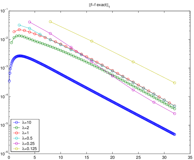
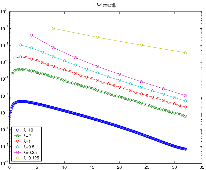
The numerical test is an homogeneous relaxation problem in the two dimensional velocity space. The molecules are Maxwellian and a fast spectral method [10] is used to compute the collision operator with $N_{v}=64$ grid points in each velocity direction and a grid $[-v_{\max},v_{\max}]^{2}$ with $v_{\max}=3\pi$ . In this case, the exact solution is given by

f(v,t)=\frac{1}{2\pi S^{2}\sigma^{2}}\left(2S-1+\frac{1-S}{2S}\frac{v^{2}}{\sigma^{2}}\right)\exp\left(-\frac{v^{2}}{2S\sigma^{2}}\right),\qquad S(t)=1-\frac{\exp\left(-\sigma^{2}t/8\right)}{2},

where we took $\sigma=1$ . The figure 1 shows the error of the schemes for different choices of the time step $\Delta t$ (stability condition for the explicit Euler scheme is $\Delta t=1$ ). We can clearly observe the expected accuracy of the schemes even for large time steps.

\begin{array}[]{c|ccccc}0&0&0&0&0\\ 0&0&0&0&0\\ 1&0&1&0&0\\ 1&0&1/2&1/2&0\\ \hline\cr&0&1/2&1/2&0\end{array}\hskip 18.49988pt\begin{array}[]{c|ccccc}2&2&0&0&0\\ 0&-2&2&0&0\\ 1&0&-1&2&0\\ 1&0&1/2&-3/2&2\\ \hline\cr&0&1/2&-3/2&2\end{array}

Table 1: Tableau of the second order IMEX-BE(2,2,4) asymptotic and positivity preserving IMEX scheme.

\begin{array}[]{c|cccccc}0&0&0&0&0&0\\ 1&1&0&0&0&0\\ 2/3&4/9&2/9&0&0&0\\ 1&1/4&0&3/4&0&0\\ 1&1/4&0&3/4&0&0\\ \hline\cr&1/4&0&3/4&0&0\end{array}\hskip 18.49988pt\begin{array}[]{c|cccccc}0&0&0&0&0&0\\ 1&1/2&1/2&0&0&0\\ 2/3&5/18&-1/9&1/2&0&0\\ 1&1/2&0&0&1/2&0\\ 1&1/4&0&3/4&-1/2&1/2\\ \hline\cr&1/4&0&3/4&-1/2&1/2\end{array}

Table 2: Tableau of the third order IMEX-BE(3,5,5) globally stiffly accurate IMEX scheme.

Acknowledgement. G. Dimarco was supported by the French ANR project BOOST.

References

[1] M. Bennoune, M. Lemou, L. Mieussens, Uniformly stable numerical schemes for the Boltzmann equation preserving the compressible Navier-Stokes asymptotics, J. Comp. Phys., 227 (2008), pp. 3781–3803.
[2] S. Boscarino, L. Pareschi, G. Russo,Implicit-Explicit Runge-Kutta schemes for hyperbolic systems and kinetic equations in the diffusion limit, Preprint, (2011)
[3] S. Boscarino, G. Russo, On a class of uniformly accurate IMEX Runge-Kutta schemes and applications to hyperbolic systems with relaxation, SIAM J. Sci. Comp. 31, (2009), pp. 1926–1945.
[4] G. Dimarco, L. Pareschi., Exponential Runge-Kutta methods for stiff kinetic equations., SIAM J. Num. Anal. 49, (2011), pp. 2057–2077.
[5] G. Dimarco, L. Pareschi., Asymptotic-Preserving IMEX Runge-Kutta methods for nonlinear kinetic equations, preprint, (2012)
[6] F. Filbet, S. Jin, A class of asymptotic preserving schemes for kinetic equations and related problems with stiff sources, J. Comp. Phys. 229, (2010), pp. 7625Ð-7648.
[7] E. Gabetta, L. Pareschi, G. Toscani, Relaxation schemes for nonlinear kinetic equations, SIAM J. Numer. Anal., 34 (1997), pp. 2168–2194.
[8] S. Jin, Efficient Asymptotic-Preserving (AP) schemes for some multiscale kinetic equations, SIAM J. Sci. Comput., 21 (1999), pp. 441–454.
[9] M. Lemou, Relaxed micro-macro schemes for kinetic equations, C. R. Acad. Sci. Paris, Ser. I, 348 (2010), pp. 455–460.
[10] C. Mouhot, L. Pareschi, Fast algorithms for computing the Boltzmann collision operator, Math. Comp. 75 (2006), pp. 1833–1852
[11] L. Pareschi, G. Russo, Implicit-Explicit Runge-Kutta methods and applications to hyperbolic systems with relaxation, J. Sci. Comput., 25 (2005), pp. 129–155.