Weak Galerkin methods for second order elliptic interface problems
Abstract
Weak Galerkin methods refer to general finite element methods for partial differential equations (PDEs) in which differential operators are approximated by their weak forms as distributions. Such weak forms give rise to desirable flexibilities in enforcing boundary and interface conditions. A weak Galerkin finite element method (WG-FEM) is developed in this paper for solving elliptic PDEs with discontinuous coefficients and interfaces. The paper also presents many numerical tests for validating the WG-FEM for solving second order elliptic interface problems. For such interface problems, the solution possesses a certain singularity due to the nonsmoothness of the interface. A challenge in research is to design high order numerical methods that work well for problems with low regularity in the solution. The best known numerical scheme in the literature is of order for the solution itself in norm. It is demonstrated that the WG-FEM of lowest order is capable of delivering numerical approximations that are of order in the usual norm for or Lipschitz continuous interfaces associated with a or continuous solution. Theoretically, it is proved that high order of numerical schemes can be designed by using the WG-FEM with polynomials of high order on each element.
keywords
Finite element methods, weak Galerkin method, second order elliptic interface problems, nonsmooth interface, low solution regularity.AMS
Primary, 65N15, 65N30, 76D07; Secondary, 35B45, 35J501 Introduction
In this paper, we are concerned with interface problems for second order elliptic partial differential equations (PDEs) with discontinuous coefficients and singular sources. For simplicity, consider the model problem of seeking functions and satisfying
| (1) | |||||
| (2) | |||||
| (3) | |||||
| (4) | |||||
| (5) | |||||
| (6) |
where , , and and are outward normals of and . Here, and can be singular and may be of Lipschitz continuous. This problem is commonly referred to as an elliptic interface problem and occurs widely in practical applications, such as fluid mechanics [23], electromagnetic wave propagation [14, 18, 41, 40], materials science [20, 22], and biological science [39, 12, 7]. The finite difference based solution of elliptic interface problems was pioneered by Peskin with his immersed boundary method (IBM) in 1977 [30, 29]. Mayo constructed an interesting integral equation approach to this class of problems [25]. To properly solve the elliptic interface problem, one needs to enforce additional interface conditions (5) and (6). LeVeque and Li advanced the subject with their second order sharp interface scheme, the immersed interface method (IIM) [24]. In the past decades, many other elegant methods have been proposed, including the ghost fluid method (GFM) proposed by Fedkiw, Osher and coworkers [11], finite-volume-based methods [28], the piecewise-polynomial discretization [8], and matched interface and boundary (MIB) method [41, 43, 37].
A proof of second order convergence of the IIM for smooth interfaces was due to Beale and Layton [2]. Rigorous convergence analysis of most other finite difference based elliptic interface schemes is not available yet. In general, it is quite difficult to analyze the convergence of finite difference based interface schemes because conventional techniques used in Galerkin formulations are not applicable for collocation schemes. The analysis becomes particularly difficult when the designed elliptic interface scheme is capable of dealing with nonsmooth interfaces [37]. At present, there is no rigorous convergence analysis available for elliptic interface methods that deliveries high-order accuracy for nonsmooth interfaces, to the author’s knowledge.
Finite element methods (FEMs) are another class of important approaches for elliptic interface problems. The construction of FEM solutions to elliptic interface problems dates back to 1970s [1], and has been a subject of intensive investigation in the past few decades [10, 31, 17, 6]. Since the elliptic interface problem defined in Eqs. (1)-(6) provides opportunities to construct new FEM schemes, a wide variety of FEM approaches have been proposed in the literature. There are two major classes of FEM based interface methods, namely, interface-fitted FEMs and immersed FEMs, categorized according to the topological relation between discrete elements and the interface. In the interface-fitted FEMs, or body-fitted FEMs, the finite element mesh is designed to align with the interface. Local mesh refinement based priori and/or posteriori error estimation can be easily carried out. The performance of interface-fitted FEMs depends on the quality of the element mesh near the interface as well as the formulation of the problem. In fact, the construction of high quality FEM meshes for real world complex interface geometries is an active area of research. Bramble and King discussed a FEM for nonhomogeneous second order elliptic interface problems on smooth domains [4]. One way to deal with embedded interface conditions is to use distributed Lagrange multipliers [5], In fact, similar ideas have been widely used in mortar methods and fictitious domain methods for the treatment of embedded boundaries [13]. A -nonconforming finite element method was also proposed for elliptic interface problems [31]. Discontinuous Galerkin (DG) FEMs have been developed for elliptic equations with discontinuous coefficients [9, 17]. Inherited from the original DG method, DG based interface schemes have the flexibility to implement interface jump conditions.
Immersed FEMs are also effective approaches for embedded interface problems [10, 35, 15, 21, 16]. A key feature of these approaches is that their element meshes are independent of the interface geometry, i.e., the interface usually cuts through elements. As such, there is no need to use the unstructured mesh to body-fit the interface, and simple structured Cartesian meshes can be employed in immersed FEMs. Consequently, the time-consuming meshing process is bypassed in immersed FEMs. However, to deal with complex interface geometries, it is necessary to design appropriate interface algorithms, which is similar to finite-difference based elliptic interface methods. In fact, immersed FEMs can be regarded as the Galerkin formulations of finite difference based interface schemes. It is not surprised that key ideas of many immersed FEMs actually come from the corresponding finite-difference based interface schemes. Additionally, other ideas in numerical analysis have been utilized for the construction of immersed FEMs. For example, a stabilized Lagrange multiplier method based on Nitsche technique has been used to enforce interface jump constraints [16]. The performance of immersed FEMs depends on the design of elegant interface schemes for complex interface geometries.
Convergence analysis of FEM based elliptic interface methods has been considered by many researchers. Unlike the collocation formulation, the Galerkin framework of FEMs allows more rigorous and robust convergence analysis. Cai el al gave a proof of convergence for a DG FEM for interface problems [6]. Dryja et al discussed the convergence of the DG discretization of Dirichlet problems for second-order elliptic equations with discontinuous coefficients in 2D [9]. Hiptmair et al presented a convergence analysis of -elliptic interface problems in general 3D Lipschitz domains with smooth material interfaces [19]. Recently, an edge-based anisotropic mesh refinement algorithm has been analyzed and applied to elliptic interface problems [33].
Despite of numerous advancements in the numerical solution of interface problems, there are still a few remaining challenges in the field. One of these challenges concerns the construction of higher order interface schemes. Currently, most interface schemes are designed to be of second order convergence. However, higher order methods are efficient and desirable for problems associated with high frequency waves, such as electromagnetic and acoustic wave propagation and scattering, vibration analysis of engineering structures, and shock-vortex interaction in compressible fluid flows. It is easy to construct high order methods and even spectral methods for these problems with straight interfaces in simple domains. However, it is extremely difficult to obtain high order convergence when the interface geometries are arbitrarily complex. A fourth order MIB scheme has been developed for the Helmholtz equation in media with arbitrarily curved interfaces in 2D [40]. Up to sixth order MIB schemes have been constructed for the Poisson equation with ellipsoidal interfaces in 3D [37]. There are two standing open problems concerning high order elliptic interface schemes, i.e., the construction of fourth-order 3D interface schemes for arbitrarily complex interfaces with sharp geometric singularities and the construction of sixth-order 3D interface schemes for arbitrarily curved smooth interfaces [37].
Another challenging issue in elliptic interface problems arises from nonsmooth interfaces or interfaces with Lipschitz continuity [39, 38, 36, 21]. Nonsmooth interfaces are also referred to as geometric singularities, such as sharp edges, cusps and tips, which commonly occur in real-world applications. It is a challenge to design high order interface schemes for geometric singularities both numerically and analytically. The first known second order accurate scheme for nonsmooth interfaces was constructed in 2007 [38]. Since then, many other interesting second order schemes have been constructed for this class of problems in 2D [8, 21, 3] and 3D [37]. The second order MIB method for 3D elliptic PDEs with arbitrarily non-smooth interfaces or geometric singularities has found its success in protein electrostatic analysis [39, 12, 7]. However, it appears truly challenging to develop fourth order schemes for arbitrarily shaped nonsmooth interfaces in 3D domains, although fourth order schemes have been reported for a few special interface geometries [37]. Due to the need in practical applications, further effort in this direction is expected.
The above mentioned difficulties in the solution of interface problems with geometric singularities significantly deteriorate in certain physical situations. It is well-known that the electric field diverges near the geometric singularities, such as tips of electrodes, antenna and elliptic cones, and sharp edges of planar conductors. Since electric field is related to the gradient of the electrostatic potential, i.e., the solution of the Poisson equation in the electrostatic analysis, it turns out that the solution of the elliptic equation has a lower regularity, e.g., the gradient does not exist at the geometric singularities. For isolated singularities, one can alleviate the difficulty by introducing an algebraic factor to solve a regularized equation whose solution has a high regularity [39, 36]. In this manner, second order MIB schemes have been constructed in the past [39, 36]. However, it is also desirable to directly solve the original PDEs with a low solution regularity. The FEM developed by Hou et al is of first order convergence in the solution and 0.7th order convergence in the gradient of the solution when the solution of the Poisson equation is or continuous and the interface is Lipschitz continuous [21]. In fact, due to the low solution regularity induced by the nonsmooth interface, it is very difficult to analyze the convergence of numerical schemes because commonly used techniques may no longer be available. Therefore, there is a pressing need to develop both high order numerical methods and rigorous analysis of numerical methods for elliptic interface problems with low solution regularities induced by geometric singularities.
The objective of the present work is to construct a new numerical method for elliptic equations with low solution regularities induced by nonsmooth interfaces. To this end, we employ a newly developed weak Galerkin finite element method (WG-FEM) by Wang and Ye [34]. Like the discontinuous Galerkin (DG) methods, WG-FEM makes use of discontinuous functions in the finite element procedure which endows WG-FEMs with high flexibility to deal with geometric complexities and boundary conditions. For interface problems, such a flexibility gives rise to robustness in the enforcement of interface jump conditions. Unlike DG methods, WG-FEM enforces only weak continuity of variables naturally through well defined discrete differential operators. Therefore, weak Galerkin methods avoid pending parameters resulted from the excessive flexibility given to individual elements. As a consequence, WG-FEMs are absolutely stable once properly constructed. Recently, WG-FEMs have been applied to the solution of second-order elliptic equations [26], and the solution of Helmholtz equations with large wave numbers [27]. A major advantage of the present weak formulation is that it naturally enables WG-FEM to handle interface problems with low solution regularities. We demonstrate that the present WG-FEM of lowest order is able to achieve from th order to second order of convergence in the solution and about first order of convergence in the gradient when the solution of the elliptic equation is or continuous and the interface is or Lipschitz continuous.
The rest of this paper is organized as follows. Section 2 is devoted to a description of the method and algorithm. We shall design a weak Galerkin formulation for the elliptic interface problem given in Eqs. (1)-(6). Section 3 is devoted to a convergence analysis for the weak Galerkin scheme presented in Section 2. In Section 4, we shall present some numerical results for several test cases in order to demonstrate the performance of the proposed WG-FEM for elliptic interface problems in 2D. We first consider a few popular benchmark test examples with smooth but complex interfaces. We then carry out some investigation about nonsmooth interfaces. Some of these test problems admit solutions with low regularities, for which our numerical results significantly improve the best known result in literature and are better than our theoretical prediction. This paper ends with a conclusion, especially a remark on the use and possible advantages of high order WG-FEMs.
2 Methods and Algorithms
Let be a partition of the domain with mesh size . We require that the edges of the elements in align with the interface . Thus, the partition can be grouped into two sets of elements denoted by and , respectively. Observe that provides a finite element partition for the subdomain . The intersection of the partition also introduce a finite element partition for the interface , which shall be denoted by . For simplicity, we adopt the following notation:
For each triangle , let and denote the interior and boundary of respectively. Denote by the set of polynomials in with degree no more than , and the set of polynomials on each segment (edge or face) , with degree no more than . A discrete function refers to a polynomial with two components in which the first component is associated with the interior and is defined on each edge or face , . Please note that may or may not equal to on . Now we introduce three trial finite element spaces as follows
| (7) | |||||
| (8) | |||||
| (9) |
Define two test spaces by
and
For each or , we define the discrete gradient of , denoted by on each element , by the following equation:
| (10) |
where is a subspace of the set of vector-valued polynomials of degree no more than on .
The selection of the indices , , , and is critical in the design of weak Galerkin finite element methods. A detailed discussion on the selection of those indices can be found in [34]. In the present study of the interface problem, we shall let in (7)-(9) and chose the Raviart-Thomas element for . These elements are referred as element in our numerical experiments. An exploration of other possible combinations is left to interested readers for future research. Recall that the Raviart-Thomas element [32] of order is of the following form
where is the set of homogeneous polynomials of degree and .
3 Convergence Theory
The goal of this section is to provide a convergence theory for the weak Galerkin finite element method as described in the previous section. First, we show that the WG algorithm has one and only one solution in the corresponding finite element trial space.
Proof.
It suffices to show that the solution of (11)-(13) is trivial when data is homogeneous; i.e., . To this end, by letting in (13) and then using the assumption of we obtain on . Next, by first letting in (11) and in (12) and then adding them up gives
which implies and . Thus, both and are constants over and , respectively. It follows from the assumption of on the non-empty set that . Thus, we have on , which together with implies . Finally, using and letting on any edge/face , we have from equation (11) that
which implies . ∎
Denote by a local projection operator where:
are the usual projections into the corresponding spaces. Let be the usual projection operator in the mixed finite element method such that ; and on each , one has satisfying
Lemma 2.
Let be a smooth vector-valued function and be the locally defined projection operator commonly used in the mixed finite element method. Then, the following identify holds true
| (14) |
for any with or and .
Proof.
It follows from the definition of and that
Now using the continuity of across each interior edge or face we arrive at
where we have used the fact that and on . This completes the proof. ∎
The following error estimates are straightforward from the definition of and . Readers can also find a verification of the result in [34].
Lemma 3.
For and with , we have
| (15) | |||||
| (16) |
It is well known that there exists a constant such that for any function
| (17) |
where is an edge of .
Theorem 4.
Proof.
For simplicity, we assume that the coefficient is a constant tensor on each element . The proof can be extended to the general case of non-constant tensor without any difficulty.
Now testing (1) with and then using (14) leads to
Adding the term to both sides of the equation above, we obtain
| (20) | |||||
Similarly, on we have for any the following relation
| (21) | |||||
Using the interface condition (6), we from from (21) that
| (22) | |||||
Testing the interface condition (5) by implies
| (23) |
For simplicity, we introduce the following notations to represent the errors:
Thus, the difference of (20) and (11) gives
| (24) |
The difference of (22) and (12) gives
| (25) |
The difference of (23) and (13) gives
| (26) |
First letting and in (24) and (25) and then adding them up gives
Using (15)-(16), we have from the above equation that
which implies
| (27) |
Using (17) and the inverse inequality, we have for any edge or face
| (28) | |||||
| (29) |
Choosing in equation (24) such that for all and for and otherwise yields
Using (10), the equation above becomes
Using (28), (29), (15) and (18), we have
which verifies the error estimate (19). This completes the proof of the theorem. ∎
4 Numerical experiments
The goal of this section is to numerically validate the proposed WG algorithm by solving some benchmark elliptic interface problems for which analytical solutions are known. To fully demonstrate the accuracy and robustness of the WG method, we consider challenging problems involving Lipschitz continuous interfaces, highly oscillated solutions, and solutions with low regularities. For simplicity, we use the piecewise constant finite element on structured triangular meshes in all test cases. The mesh generation and computation are all conducted in the MATLAB environment. Since the analytical solutions are known for each test case, the nonhomogeneous terms and of the elliptic equations and the Dirichlet boundary data can be correspondingly derived. Moreover, the two interface jump conditions for the solution and the flux across the interface are calculated according to the given analytical solution. Numerical errors in the solution and its gradient are reported in norms in all examples.
| Mesh | Solution | Gradient | |||
|---|---|---|---|---|---|
| error | order | error | order | ||
| Level 1 | 2.8553e-01 | 1.0266e-02 | 1.3042e-02 | ||
| Level 2 | 1.5110e-01 | 2.9631e-03 | 1.9525 | 6.5234e-03 | 1.0886 |
| Level 3 | 7.7543e-02 | 7.6763e-04 | 2.0247 | 3.2615e-03 | 1.0391 |
| Level 4 | 3.9258e-02 | 1.9518e-04 | 2.0118 | 1.6306e-03 | 1.0185 |
| Level 5 | 1.9749e-02 | 4.9198e-05 | 2.0058 | 8.1523e-04 | 1.0090 |
|
Example 1. We first study a classical circular interface problem [42]. Consider a square domain with a circular interface . The coefficient is defined to be and , respectively on each subdomain, for and . The analytical solution to the elliptic equation is given as
By choosing , the function and flux jumps are actually constants [42].
By using a uniform triangular mesh, the error for the solution and its gradient of the WG method is reported in Table 1. Based on successive mesh refinements, the numerically detected convergence rates are also reported for both error measurements. It can be seen that the orders of convergence in norm for the solution and gradient are, respectively, two and one for piecewise constant WG finite element approximations. This agrees with our theoretical results.
In Fig. 1, the WG solutions based on mesh levels 1 and 5 are depicted. By using piecewise constant finite elements, the WG solution at mesh level 1 clearly consists of piecewise constants. On the other hand, a much better numerical solution is attained at mesh level 5. It is also seen that the function and flux jumps are constant across the circular interface.
| Mesh | Solution | Gradient | |||
|---|---|---|---|---|---|
| error | order | error | order | ||
| Level 1 | 3.1778e-01 | 7.6628e-02 | 1.5852e-01 | ||
| Level 2 | 1.5889e-01 | 1.5119e-02 | 2.3415 | 5.2258e-02 | 1.6009 |
| Level 3 | 7.9444e-02 | 3.6142e-03 | 2.0646 | 2.0731e-02 | 1.3338 |
| Level 4 | 3.9722e-02 | 8.9375e-04 | 2.0157 | 9.6505e-03 | 1.1031 |
| Level 5 | 1.9861e-02 | 2.2492e-04 | 1.9905 | 4.7340e-03 | 1.0275 |
| Mesh | Solution | Gradient | |||
|---|---|---|---|---|---|
| error | order | error | order | ||
| Level 1 | 1.5837e-01 | 8.6774e-01 | 5.2751e+00 | ||
| Level 2 | 7.9186e-02 | 1.4156e-01 | 2.6159 | 9.1695e-01 | 2.5243 |
| Level 3 | 3.9593e-02 | 2.3768e-02 | 2.5743 | 2.8679e-01 | 1.6768 |
| Level 4 | 1.9796e-02 | 5.8719e-03 | 2.0170 | 1.0732e-01 | 1.4180 |
| Level 5 | 9.8982e-03 | 1.4717e-03 | 1.9964 | 4.7255e-02 | 1.1834 |


|
Example 2. To further explore the potential of the proposed WG method, we consider a circular interface problem with highly oscillatory solutions. The high frequency or short wave solutions are commonly encountered in solving electromagnetic wave propagation and scattering problems governed by time domain Maxwell’s equations or frequency domain Helmholtz equations. Here, we consider the following Helmholtz interface problem [42]
| (30) | |||||
| (31) |
where the interface is still over the domain . The wavenumber () depends on the wavenumber of the wave solution in free space and dielectric profiles . In the present example, both and are chosen to be discontinuous across the interface. In particular and for and and for . The analytical solution is given as
Other necessary interface jump conditions can be derived from the analytical solution.
The WG solution of the Helmholtz equation with high wavenumbers has been explored in [27]. For the present Helmholtz interface problem, a WG algorithm can be similarly constructed based on equations (11) - (13). Two frequencies are tested, i.e., and , and the results are reported in Tables 2 and 3. By using , the solution is of high frequency, see Fig. 2. In comparison with the numerical accuracy of the WG method for both cases, the WG errors for are larger even though a finer mesh is employed in the same mesh level. Nevertheless, when we examine the convergence rates, the WG method maintains the same rates, i.e., second and first orders, respectively, for the solution and its gradient, in both cases. This verifies the capability of the WG method in resolving short wave solutions.
| Mesh | Solution | Gradient | |||
|---|---|---|---|---|---|
| error | order | error | order | ||
| Level 1 | 5.6522e-01 | 1.4339e-01 | 1.5956e-01 | ||
| Level 2 | 2.8261e-01 | 2.6979e-02 | 2.4100 | 9.1557e-02 | 0.8014 |
| Level 3 | 1.4130e-01 | 7.3332e-03 | 1.8792 | 5.8167e-02 | 0.6544 |
| Level 4 | 7.0652e-02 | 1.4904e-03 | 2.2988 | 2.9623e-02 | 0.9735 |
| Level 5 | 3.5326e-02 | 2.8124e-04 | 2.4058 | 1.5250e-02 | 0.9579 |

|
| Mesh | Solution | Gradient | |||
|---|---|---|---|---|---|
| error | order | error | order | ||
| Level 1 | 5.6522e-01 | 4.1482e-01 | 3.1081e-01 | ||
| Level 2 | 2.8261e-01 | 5.3753e-02 | 2.9481 | 1.0784e-01 | 1.5271 |
| Level 3 | 1.4130e-01 | 1.3707e-02 | 1.9713 | 5.6088e-02 | 0.9431 |
| Level 4 | 7.0652e-02 | 3.0677e-03 | 2.1598 | 2.9658e-02 | 0.9193 |
| Level 5 | 3.5326e-02 | 6.2057e-04 | 2.3055 | 1.5204e-02 | 0.9640 |

|
Example 3. We next consider an example with a high contrast in coefficient [42] to examine the robustness of the WG method. Consider the second order elliptic equation over the domain . The interface is defined to be an ellipse
We set inside of , and outside of . The analytical solution is given as
Other necessary conditions can be derived from the analytical solution.
Two values of are tested with and . The latter case involves a much larger jump in . This results in a larger condition number for the corresponding discretized linear system. This means that extensive computational time is usually needed in the matrix solving. The WG method performs robustly for both cases. The numerical results are presented in Table 4 and Table 5, respectively, for and . It can be seen in both tables that the convergence rates are first and second orders, respectively, for the gradient and the solution in norm. The WG solutions on mesh levels 1 and 5 are shown in Fig. 3 and Fig. 4, respectively, for and . We note that in both cases, the analytical solutions are the same and are independent of the coefficient . Thus, even though there are some minor differences in the WG solutions at mesh level 1 for and , the WG solutions are visually identical at mesh level 5. This demonstrates the robustness of the WG method in handling interface problems with high contrast.
| Mesh | Solution | Gradient | |||
|---|---|---|---|---|---|
| error | order | error | order | ||
| Level 1 | 3.4726e-01 | 1.5885e-03 | 3.5260e-02 | ||
| Level 2 | 1.7363e-01 | 3.8053e-04 | 2.0616 | 1.6630e-02 | 1.0842 |
| Level 3 | 8.9010e-02 | 9.1082e-05 | 2.1399 | 9.0379e-03 | 0.9126 |
| Level 4 | 4.9602e-02 | 2.6778e-05 | 2.0936 | 5.0265e-03 | 1.0034 |
| Level 5 | 2.4286e-02 | 5.9847e-06 | 2.0982 | 2.4459e-03 | 1.0087 |

|
|
|
|
|
Example 4. We next consider a classical elliptic interface problem with both concave and convex curve segments [42]. The interface is parametrized with the polar angle
inside a square domain . The coefficient is chosen to be and , respectively, for outside and inside . The analytical solution is given as
Other necessary interface jump conditions can be derived from the analytical solutions.
The WG solutions and their convergence are reported in Table 6 and Fig. 5, respectively. It can be seen from the table that the convergence is of order two and one for the solution and its gradient, respectively, in the norm. It should be pointed out that mesh quality plays an important role in the performance of general finite element methods. For weak Galerkin, we noted that the quality of mesh affects the corresponding numerical approximation in norms. For example, we noted a slower convergence when the finite element partition consists of both acute and non-acute triangles with nontrivial portion. After eliminating most of the non-acute triangles, the WG approximation exhibits an improved rate of convergence numerically. Figure 6 demonstrates some meshes generated by MATLAB in the present study after an elimination of most non-acute triangles through a numerical procedure. It can be seen that, at each level, the triangular mesh is fitted to the interface at the nodal points. Observe that these meshes are highly non-uniform and unstructured. In particular, it is clear that much smaller triangles are employed to resolve the concave portion of the interface. This somehow helped the WG method to deliver numerical solutions with high accuracy since the solution changes rapidly in regions with large curvatures.
| Mesh | Solution | Gradient | |||
|---|---|---|---|---|---|
| error | order | error | order | ||
| Level 1 | 6.2575e-01 | 1.5275e-02 | 4.8833e-02 | ||
| Level 2 | 2.9662e-01 | 3.9259e-03 | 1.8200 | 3.1059e-02 | 0.6062 |
| Level 3 | 1.5170e-01 | 1.0586e-03 | 1.9546 | 1.5584e-02 | 1.0285 |
| Level 4 | 7.9102e-02 | 3.3419e-04 | 1.7707 | 8.0209e-03 | 1.0200 |
| Level 5 | 4.4180e-02 | 1.1698e-04 | 1.8022 | 4.4282e-03 | 1.0199 |

|
Example 5. In this and next two examples, we consider an interface problem with continuous interfaces as discussed in [21]. The domain is given as , and the interface is defined with two pieces: for and , for . The interface divides the domain into two parts and . Here we denote and , respectively, to be the part on the left and right of . An inhomogeneous second order elliptic equation is considered, i.e., the coefficient is not piecewise constant. Instead, we have in and in . The analytical solution is fixed to be in , while in , is defined piecewisely by
Other necessary conditions can be derived from the analytical form of the solution. In particular, the Dirichlet boundary data is derived for both and , since in this example, is not enclosed by .
A numerical investigation was conducted and the results are reported in Table 7. Again, the WG method attains the theoretical order of convergence for this example, i.e., first and second order of accuracy respectively for the gradient and the solution in norm. We note that due to the piecewise definition, the solution is continuous but not across the line . In our computation, the line is not treated as a boundary. Thus, our triangulation is not aligned with this line. This can be seen clearly in the graph of the WG solution on mesh level 1 (Fig. 7 left). In the right chart of Fig. 7, a smooth transition can be seen across in the WG solution on mesh level 5.
| Mesh | Solution | Gradient | |||
|---|---|---|---|---|---|
| error | order | error | order | ||
| Level 1 | 6.2575e-01 | 2.6559e-02 | 4.9273e-02 | ||
| Level 2 | 2.9662e-01 | 5.9674e-03 | 2.0001 | 2.8456e-02 | 0.7355 |
| Level 3 | 1.5170e-01 | 1.5342e-03 | 2.0257 | 1.4493e-02 | 1.0062 |
| Level 4 | 7.9102e-02 | 4.4127e-04 | 1.9137 | 7.5081e-03 | 1.0100 |
| Level 5 | 4.4180e-02 | 1.5022e-04 | 1.8500 | 3.9584e-03 | 1.0990 |

|
Example 6. Here we consider the same interface and domain geometry as in Example 5. The coefficient function is defined in the same way as in Example 5. We also fix the solution as in . But in , the solution is given differently by (see [21] for details)
Other necessary conditions can be derived similarly. Observe that the solution is continuous but not across the line .
The WG algorithm is formulated as in the previous example. In particular, since is across , the function and flux jumps are trivially zero across . Thus, again, no special boundary or interface treatment is carried out near the line . In fact, this line actually cuts through the finite element triangles; see the left chart of Fig. 8. It can be seen that the loss of regularity in is visually indistinguishable in the WG solution on mesh level 5 (see the right chart of Fig. 8). In literature, a certain reduction of convergence order has been reported for this continuous example [21] when the standard Galerkin finite element method is employed for a numerical approximation. In the present study, it is found that the order of convergence remains unchanged for the WG method, see Table 8. This indicates that the WG method preforms robustly for the challenging problem with low regularity.
| Mesh | Solution | Gradient | |||
|---|---|---|---|---|---|
| error | order | error | order | ||
| Level 1 | 6.5801e-01 | 3.4340e-02 | 3.2817e-01 | ||
| Level 2 | 3.4551e-01 | 1.1022e-02 | 1.7641 | 1.7896e-01 | 0.9413 |
| Level 3 | 1.7932e-01 | 3.5197e-03 | 1.7405 | 9.5039e-02 | 0.9650 |
| Level 4 | 9.1176e-02 | 1.0806e-03 | 1.7459 | 5.0095e-02 | 0.9468 |
| Level 5 | 4.6365e-02 | 3.3092e-04 | 1.7499 | 2.6003e-02 | 0.9696 |

|
Example 7. Consider again the same interface problem as in Examples 5 and 6, over a larger domain . The coefficient function is now defined to be in and in . The analytical solution is give as [21]
Other necessary conditions can be derived from the analytical solutions.
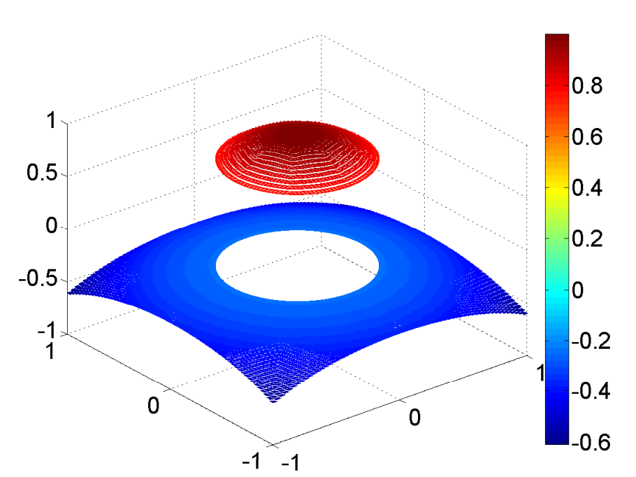
The analytical solution is piecewise in this example. In particular, the function has a singularity at with blow-up derivatives. Even though the analytical solution is well behaved in other places, the singularity at the origin may cause some order reduction in the finite element simulation [21]. Due to this singularity, the convergence rate of the WG method in the norm of the solution is reduced to be about for the present example, see Table 9. On the other hand, the order of convergence for the WG method for the gradient remains to be about one. The numerical solutions at mesh levels 1 and 5 are depicted in Fig. 9. Interestingly, in both levels, the singularity at the origin is invisible. But the numerical algorithm can sense this singularity via the convergence rate.
| Mesh | Solution | Gradient | |||
|---|---|---|---|---|---|
| error | order | error | order | ||
| Level 1 | 5.6919e-01 | 1.4984e-02 | 3.3001e-02 | ||
| Level 2 | 2.8459e-01 | 4.4307e-03 | 1.7578 | 1.7812e-02 | 0.8897 |
| Level 3 | 1.4230e-01 | 1.2336e-03 | 1.7687 | 9.8402e-03 | 0.8561 |
| Level 4 | 7.1149e-02 | 3.2639e-04 | 1.8634 | 5.1905e-03 | 0.9228 |
| Level 5 | 3.5574e-02 | 8.5110e-05 | 1.9231 | 2.6699e-03 | 0.9591 |

|
Example 8. In this and next two examples, we continue to examine the performance of the WG method for solutions of low regularity when the interface is fixed to be a Lipschitz continuous curve[21]. On a rectangular domain , we consider a case where the interface consists of two pieces: for and , for . Thus, the interface has a kink at . Denote by the region on the left and upper part of , and to be the rest of the domain. The coefficient is given piecewisely by in and in . The analytical solution is fixed to be in , while in , is given piecewisely by
Other necessary conditions can be derived from the analytical solutions.
Similar to Example 5, the analytical solution is of continuous but not in this example. The WG method yields uniformly second and first order of accuracy in norm, respectively, for the solution and its gradient as shown in Table 10. The kink of the interface is clearly seen in both charts of Fig. 10. In particular, on the coarsest mesh, the alignment of finite element triangles to two line segments of is obvious. No deterioration in solution occurs around the interface corner.
| Mesh | Solution | Gradient | |||
|---|---|---|---|---|---|
| error | order | error | order | ||
| Level 1 | 5.6919e-01 | 1.4326e-02 | 3.3514e-02 | ||
| Level 2 | 2.8459e-01 | 4.4250e-03 | 1.6949 | 2.0051e-02 | 0.7411 |
| Level 3 | 1.4230e-01 | 1.2350e-03 | 1.8411 | 1.0768e-02 | 0.8968 |
| Level 4 | 7.1149e-02 | 3.2693e-04 | 1.9175 | 5.5458e-03 | 0.9573 |
| Level 5 | 3.5574e-02 | 8.5118e-05 | 1.9415 | 2.8004e-03 | 0.9858 |

|
Example 9. Consider an elliptic problem with the same interface and domain geometry as in Example 8. The coefficient function is defined the same as in Example 8. Also, we fix the solution to be in . But in , the solution is given differently [21] by
Other necessary conditions can be derived similarly. Like in Example 6, is of continuous but not across the line . Similarly, no special numerical treatment is invoked near the line so that this line actually cuts through finite element triangles, see the left chart of Fig. 11. It can be seen from Table 11 that the WG method converges uniformly with orders being close to second and first, respectively, for the solution and its gradient in the norm. Technically speaking, the interface is Lipschitz continuous in this example, while it is continuous in Example 6. In other words, the interface regularity is lower here than that in Example 6. However, since body-fitted triangular meshes are employed in the WG method, the interface with two simple line segments in the present example is easier to be resolved by the body-fitted grids than the curved interface in Example 6. The only issue that could make an impact on the convergence is the geometrical singularity at the origin. The last and present examples show that the WG method is very robust in handling geometrical singularity, or sharp edged corners in general.
| Mesh | Solution | Gradient | |||
|---|---|---|---|---|---|
| error | order | error | order | ||
| Level 1 | 7.1020e-01 | 4.0630e-02 | 7.1308e-02 | ||
| Level 2 | 3.5510e-01 | 1.1389e-02 | 1.8349 | 4.0849e-02 | 0.8038 |
| Level 3 | 1.7755e-01 | 3.3569e-03 | 1.7624 | 2.1170e-02 | 0.9483 |
| Level 4 | 8.8775e-02 | 1.0150e-03 | 1.7256 | 1.0780e-02 | 0.9737 |
| Level 5 | 4.4387e-02 | 3.1128e-04 | 1.7052 | 5.5740e-03 | 0.9516 |

|
Example 10. Consider the same interface and geometry as in Examples 8 and 9. The coefficient function is now defined to be in and in . The analytical solutions are give as [21]
Other necessary conditions can be derived from the analytical solution.
Similar to Example 7, the analytical solution is piecewise in the present case. The solution has a singularity at with blow-up derivatives. The WG method achieves a similar order of accuracy as that in Example 7. In particular, it can be seen in Table 12 that the error in the solution is of order , while it remains to be about for the gradient approximation. Both function singularity and geometrical singularity are presented at the origin in this test; see the WG solutions in Fig. 12. Nevertheless, the WG method is capable of delivering decent results at mesh level 1.
| Regularity | is continuous | is Lipschitz continuous | ||
|---|---|---|---|---|
| solution | gradient | solution | gradient | |
| 1.8380 | 0.9056 | 1.8650 | 0.9069 | |
| 1.9523 | 0.9513 | 1.8487 | 0.8953 | |
| 1.7500 | 0.9558 | 1.7570 | 0.9193 | |
Finally, we would like to summarize the WG results from Example 5 to Example 10 in Table 13. In each case, an overall convergence rate is reported, which is calculated based only on mesh level 1 and level 5. It can be seen from the error of the gradient that the WG method essentially attains the first order of accuracy in all test cases. For the error of the solution, we analyze the order of the WG method case by case. When the solution is continuous, the loss of regularity has no impact on the order of convergence regardless whether the interface is continuous or Lipschitz continuous. When the solution is continuous, the WG method achieves a very good order of accuracy for continuous interface, while such order is slightly reduced when the interface is Lipschitz continuous. However, the overall order of convergence for the WG method for the latter case is still very close to two. Thus, it is fair to say that the WG method attains a second order of accuracy in norm for continuous solutions. On the other hand, the error of the WG method is always around the order of when the solution is continuous, for both and Lipschitz continuous interfaces. In other words, even though the geometrical singularity does not affect the convergence of the WG method, the function singularity may do. Nevertheless, we note that a th order for solution with low regularities is still some of the best for this class of challenging problems, to our best knowledge. Moreover, although not reported in detail in this paper, the WG method achieves the second order of accuracy in norm for the solution. Therefore, the present study demonstrates a good robustness of the WG method for solving elliptic interface problems. Readers are also encouraged to draw their own conclusions from the results reported in this paper.
5 Conclusion
The present paper presents some of the best results for solving two-dimensional (2D) elliptic partial differential equations (PDE) with low solution regularity resulted from modeling nonsmooth interfaces. The weak Galerkin finite element method (WG-FEM) of Wang and Ye [34] is introduced for this class of problems. The WG-FEM is a new approach that employs discontinuous functions in the finite element procedure to gain flexibility in enforcing boundary and interface conditions. Such a strategy is akin to that used by the discontinuous Galerkin (DG) methods. However, by enforcing only weak continuity of variables though well defined discrete differential operators, the WG-FEM is able to avoid pending parameters commonly occurred in the DG-FEMs. Like traditional FEMs, the WG-FEM employs body-fitted element meshes to represent boundaries and material interfaces. Such an approach is convenient for handling nonsmooth interfaces or geometric singularities. The convergence analysis of the present WG-FEM for elliptic interface problems is given. The validity of the WG-FEM is further tested over a large number of benchmark numerical tests with various complex interface geometries and nonsmooth interfaces. The designed second order accuracy is confirmed in our numerical experiments for problems with smooth interfaces and sufficient solution regularities.
Nonsmooth interfaces, such as sharp edges, cusps, and tips are ubiquitous both in nature and in engineering devices and structures. When nonsmooth interfaces are associated with elliptic PDEs, they result in difficulties in theoretical analysis and in the design of numerical algorithms. Unfortunately, to tackle the real-world problems, dealing with nonsmooth interfaces is non-avoidable in scientific computing. What aggravates the difficulty in error analysis and in the numerical methods is the low regularity of solution resulted from nonsmooth interfaces, which is a well-known natural phenomena called tip-geometry effects in many fields. When the interface is Lipschitz continuous and solution is or continuous, the best known result in the literature is of first order convergence in solution and order of convergence in the gradient [21]. It is demonstrated that the present WG-FEM achieves at least an order of convergence in the solution and an order of convergence in the gradient. A numerical study for high order of WG methods should be conducted for a better understanding of the method.
References
- [1] I. Babuška. The finite element method for elliptic equations with discontinuous coefficients. Computing, 5:207–213, 1970.
- [2] J. T. Beale and A. T. Layton. On the accuracy of finite difference methods for elliptic problems with interfaces. Comm. Appl. Math. Comp. Sci.,, 1:91–119, 2006.
- [3] J. Bedrossian, J. H. von Brecht, S. W. Zhu, E. Sifakis, and J. M. Teran. A finite element method for interface problems in domains with smooth boundaries and interfaces. J. Comput. Phys., 229:6405–6426, 2010.
- [4] J. Bramble and J. King. A finite element method for interface problems in domains with smooth boundaries and interfaces. Adv. Comput. Math., 6:109–138, 1996.
- [5] E. Burman and P. Hansbo. Interior-penalty-stabilized Lagrange multiplier methods for the finite-element solution of elliptic interface problems. IAM J. Numer. Anal., 30:870–885, 2010.
- [6] Z. Cai, X. Ye, and S. Zhang. Discontinuous Galerkin finite element methods for interface problems: A priori and a posteriori error estimations. SIAM J. Numer. Anal., 49:1761–1787, 2011.
- [7] D. Chen, Z. Chen, C. Chen, W. H. Geng, and G. W. Wei. MIBPB: A software package for electrostatic analysis. J. Comput. Chem., 32:657 – 670, 2011.
- [8] T. Chen and J. Strain. Piecewise-polynomial discretization and Krylov-accelerated multigrid for elliptic interface problems. J. Comput. Phys., 16:7503–7542, 2008.
- [9] M. Dryjaa, J. Galvisb, and M. Sarkisb. BDDC methods for discontinuous Galerkin discretization of elliptic problems. Journal of Complexity, 23:715–739, 2007.
- [10] R. E. Ewing, Z. L. Li, T. Lin, and Y. P. Lin. The immersed finite volume element methods for the elliptic interface problems. Mathematics and Computers in Simulation, 50:63–76, 1999.
- [11] R. P. Fedkiw, T. Aslam, B. Merriman, and S. Osher. A non-oscillatory Eulerian approach to interfaces in multimaterial flows (the ghost fluid method). J. Comput. Phys., 152:457–492, 1999.
- [12] W. H. Geng, S. N. Yu, and G. W. Wei. Treatment of charge singularities in implicit solvent models. Journal of Chemical Physics, 127:114106, 2007.
- [13] R. Glowinski, T.-W. Pan, and J. Periaux. A fictitious domain method for Dirichlet problem and applications. Computer Methods in Applied Mechanics and Engineering, 111:283–303, 1994.
- [14] G. R. Hadley. High-accuracy finite-difference equations for dielectric waveguide analysis i: uniform regions and dielectric interfaces. Journal of Lightwave Technology, 20:1210–1218, 2002.
- [15] A. Hansbo and P. Hansbo. An unfitted finite element method. Comput. Methods Appl. Mech. Engng, 191:5537-5552, 2002.
- [16] I. Harari and J. Dolbow. Analysis of an efficient finite element method for embedded interface problems. Comput. Math., 46:205–211, 2010.
- [17] X. He, T. Lin, and Y. Lin. Interior penalty bilinear IFE discontinuous Galerkin methods for elliptic equations with discontinuous coefficient. Journal of System Science and Complexity, 23:467–483, 2010.
- [18] J. S. Hesthaven. High-order accurate methods in time-domain computational electromagnetics. a review. Advances in Imaging and Electron Physics, 127:59–123, 2003.
- [19] R. Hiptmair, J. Li, and J. Zou. Convergence analysis of finite element methods for H(div;Omega)-elliptic interface problems. J. Numer. Math., 18:187–218, 2010.
- [20] T. P. Horikis and W. L. Kath. Modal analysis of circular bragg fibers with arbitrary index profiles. Optics Lett., 31:3417–3419, 2006.
- [21] S. M. Hou, W. Wang, and L. Q. Wang. Numerical method for solving matrix coefficient elliptic equation with sharp-edged interfaces. J. Comput. Phys., 229:7162-7179, 2010.
- [22] T. Y. Hou, Z. L. Li, S. Osher, and H. K. Zhao. A hybrid method for moving interface problems with application to the hele�shaw flow. J. Comput. Phys., 134(2):236–252, 1997.
- [23] A. T. Layton. Using integral equations and the immersed interface method to solve immersed boundary problems with stiff forces. Comput. Fluids., 38:266–272, 2009.
- [24] R. J. LeVeque and Z. L. Li. The immersed interface method for elliptic equations with discontinuous coefficients and singular sources. SIAM J. Numer. Anal., 31:1019–1044, 1994.
- [25] A. Mayo. The fast solution of Poisson’s and the biharmonic equations on irregular regions. SIAM J. Numer. Anal., 21:285–299, 1984.
- [26] L. Mu, J. Wang, Y. Wang, and X. Ye. A computational study of the weak Galerkin method for second-order elliptic equations. arXiv:1111.0618v1, 2011.
- [27] L. Mu, J. Wang, X. Ye, and S. Zhao. A numerical study on the weak Galerkin method for the Helmholtz equation with large wave numbers. arXiv:1111.0671v1, 2011.
- [28] M. Oevermann and R. Klein. A Cartesian grid finite volume method for elliptic equations with variable coefficients and embedded interfaces. J. Comput. Phys., 219:749–769, 2006.
- [29] C. S. Peskin and D. M. McQueen. A 3-dimensional computational method for blood-flow in the heart. 1. immersed elastic fibers in a viscous incompressible fluid. J. Comput. Phys., 81:372–405, 1989.
- [30] C. S. Peskin. Numerical analysis of blood flow in the heart. J. Comput. Phys., 25(3):220–252, 1977.
- [31] I. Ramiere. Convergence analysis of the -finite element method for elliptic problems with non-boundary-fitted meshes. Int. J. Numer. Meth. Engng, 75:10071052, 2008.
- [32] P. A. Raviart and J. M. Thomas. A mixed finite element method for 2-nd order elliptic problems, volume 606 of Mathematical Aspects of Finite Element Methods. Lecture Notes in Mathematics Series, A. Dold and B. Eckmann (Eds.), pages 292–315. Springer:Berlin, 1977.
- [33] D. A. Wang, R. Li, and N. N. Yan. An edge-based anisotropic mesh refinement algorithm and its application to interface problems. Commun. Comput. Phys., 8:511–540, 2010.
- [34] J. Wang and X. Ye. A weak Galerkin finite element method for second-order elliptic problems. arXiv:1104.2897v1, 2011.
- [35] X. S. Wang, L. T. Zhang, and L. W. Kam. On computational issues of immersed finite element methods. Journal of Computational Physics, 228:2535–2551, 2009.
- [36] K. N. Xia, M. Zhan, and G.-W. Wei. The matched interface and boundary (MIB) method for multi-domain elliptic interface problems. Journal of Computational Physics, 230:8231-8258, 2011.
- [37] S. N. Yu and G. W. Wei. Three-dimensional matched interface and boundary (MIB) method for treating geometric singularities. J. Comput. Phys., 227:602–632, 2007.
- [38] S. N. Yu, Y. Zhou, and G. W. Wei. Matched interface and boundary (MIB) method for elliptic problems with sharp-edged interfaces. J. Comput. Phys., 224(2):729–756, 2007.
- [39] S. N. Yu, W. H. Geng, and G. W. Wei. Treatment of geometric singularities in implicit solvent models. Journal of Chemical Physics, 126:244108, 2007.
- [40] S. Zhao. High order matched interface and boundary methods for the helmholtz equation in media with arbitrarily curved interfaces. J. Comput. Phys., 229:3155–3170, 2010.
- [41] S. Zhao and G. W. Wei. High-order FDTD methods via derivative matching for Maxwell’s equations with material interfaces. J. Comput. Phys., 200(1):60–103, 2004.
- [42] Y. C. Zhou and G. W. Wei. On the fictitious-domain and interpolation formulations of the matched interface and boundary (MIB) method. J. Comput. Phys., 219(1):228–246, 2006.
- [43] Y. C. Zhou, S. Zhao, M. Feig, and G. W. Wei. High order matched interface and boundary method for elliptic equations with discontinuous coefficients and singular sources. J. Comput. Phys., 213(1):1–30, 2006.