Recently new results for the structure functions $F_{L}$ and $F_{2}$ of deep inelastic electron- and positron-proton scattering (DIS) have been published by the H1 Collaboration [1]. In this note we compare these results with predictions of the popular colour-dipole model of DIS. That is, we investigate if the data respect certain bounds for the ratios of structure functions. These bounds are rigorous predictions of the dipole model and rely only on the non-negativity of the dipole-proton cross section.

The kinematics of $e^{\pm}p$ scattering is well known, see for instance [1, 2]. The reaction is

$$e^{\pm}(k)+p(p)\longrightarrow e^{\pm}(k^{\prime})+X(p^{\prime})$$

(1)

and we use the variables

	$\displaystyle q$	$\displaystyle=k-k^{\prime}=p^{\prime}-p\,,\>\>\>\>\>\>\>\>\>\>\>$	$\displaystyle Q^{2}$	$\displaystyle=-q^{2}\,,$		(2)
	$\displaystyle W^{2}$	$\displaystyle=(p+q)^{2}\,,$	$\displaystyle x$	$\displaystyle=\frac{Q^{2}}{2pq}=\frac{Q^{2}}{W^{2}+Q^{2}-m_{p}^{2}}\,.$

The measured structure functions $F_{2}$ and $F_{L}$ are related to the cross sections $\sigma_{T}$ and $\sigma_{L}$ for absorption of transversely or longitudinally polarised virtual photons by

$$\begin{split}F_{2}(x,Q^{2})&=\frac{Q^{2}}{4\pi^{2}\alpha_{\rm em}}\,(1-x)\left[\sigma_{T}(x,Q^{2})+\sigma_{L}(x,Q^{2})\right]\,,\\ F_{L}(x,Q^{2})&=\frac{Q^{2}}{4\pi^{2}\alpha_{\rm em}}\,(1-x)\,\sigma_{L}(x,Q^{2})\,.\end{split}$$

(3)

Here Hand’s convention [3] for the virtual-photon flux factor is used and terms of order $m^{2}_{p}/W^{2}$ are neglected. For low to moderate values of $Q^{2}$ the dipole picture for DIS [4, 5, 6] is frequently used to describe the data. For various applications of the dipole model see for instance [7]-[27]. In [28, 29] this dipole picture was thoroughly examined using functional methods of quantum field theory. In particular, the assumptions were spelled out which one has to make in order to arrive at the standard dipole-model formulae for $\sigma_{T}$ and $\sigma_{L}$ or, equivalently, $F_{2}$ and $F_{L}$,

$$\begin{split}F_{2}(x,Q^{2})&=\frac{Q^{2}}{4\pi^{2}\alpha_{\rm em}}\,(1-x)\sum_{q}\int\mathrm{d}^{2}r\,\left[w^{(q)}_{T}(r,Q^{2})+w^{(q)}_{L}(r,Q^{2})\right]\hat{\sigma}^{(q)}(r,\xi)\,,\\ F_{L}(x,Q^{2})&=\frac{Q^{2}}{4\pi^{2}\alpha_{\rm em}}\,(1-x)\sum_{q}\int\mathrm{d}^{2}r\,w^{(q)}_{L}(r,Q^{2})\,\hat{\sigma}^{(q)}(r,\xi)\,,\end{split}$$

(4)

see section 6 of [29]. In (4) $w^{(q)}_{T,L}$ are the probability densities for the virtual photon $\gamma^{*}$ splitting into a quark-antiquark pair of flavour $q$ and transverse separation $r$. Their standard expressions are given in Appendix A. An integration over the quark’s longitudinal momentum is performed. The cross section for the $q\bar{q}$ pair scattering on the proton is denoted by $\hat{\sigma}^{(q)}(r,\xi)$. This cross section depends on $r$ and an energy variable $\xi$ the choice of which is left open here. In [28, 29, 30, 31, 32] it was argued that the correct variable to choose is $\xi=W$. However, in the literature the energy variable used most frequently in the dipole cross section is $\xi=x$.

In the standard dipole model formulae (4) the densities $w^{(q)}_{T,L}$ are known (see Appendix A) but the dipole-proton cross sections $\hat{\sigma}^{(q)}$ have to be taken from a model. In the following we shall only use that they have to be non-negative,

$$\hat{\sigma}^{(q)}(r,\xi)\geq 0\,.$$

(5)

This alone allows to derive a non-trivial upper bound, valid in any dipole model, on the ratio

$$R(x,Q^{2})=\frac{\sigma_{L}(x,Q^{2})}{\sigma_{T}(x,Q^{2})}$$

(6)

see [29, 30]. Equivalently, one can obtain a non-trivial upper bound on the ratio

$$\frac{F_{L}(x,Q^{2})}{F_{2}(x,Q^{2})}=\frac{R(x,Q^{2})}{1+R(x,Q^{2})}\,.$$

(7)

This bound can be substantially improved if information on the charm structure function $F^{(c)}_{2}(x,Q^{2})$ is included [31]. There is then an allowed domain, again valid in any dipole model, for the two-dimensional vector

$$\vec{V}(x,Q^{2})=\begin{pmatrix}F_{L}(x,Q^{2})/F_{2}(x,Q^{2})\\ F_{2}^{(c)}(x,Q^{2})/F_{2}(x,Q^{2})\end{pmatrix}\,.$$

(8)

It is the purpose of this note to confront the dipole-model bounds on $F_{L}/F_{2}$ and on the vector $\vec{V}(x,Q^{2})$ with the new HERA results [1]. This is done in section 2. In section 3 we discuss the results, and we give a summary in section 4.

We discuss first the bound for the ratio $F_{L}/F_{2}$ of (7). For this we define

$$g(Q,r,m_{q})=\frac{w_{L}^{(q)}(r,Q^{2})}{w_{T}^{(q)}(r,Q^{2})+w_{L}^{(q)}(r,Q^{2})}\,,$$

(9)

where $m_{q}$ is the mass of the quark $q$. For the case of massless quarks, $m_{q}=0$, figure 1 shows $\frac{1}{\alpha_{\rm em}Q_{q}^{2}}(w_{T}^{(q)}+w_{L}^{(q)})(r,Q^{2})$ and $g(Q,r,0)$ as functions of $r$ for three different values of $Q=\sqrt{Q^{2}}$ (compare figure 10 of [29] for a similar plot of the function $(w_{L}^{(q)}/w_{T}^{(q)})(r,Q^{2})$).

Note that $(w_{T}^{(q)}+w_{L}^{(q)})(r,Q^{2})$ is monotonously decreasing with $r$. Its behaviour for small and large $r$ is as follows for $m_{q}=0$:

$$\begin{split}&(w_{T}^{(q)}+w_{L}^{(q)})(r,Q^{2})\propto\frac{1}{r^{2}}\>\>\>\>\>\>\mbox{for}\>\>\>\>\>\>r\to 0\,,\\ &(w_{T}^{(q)}+w_{L}^{(q)})(r,Q^{2})\propto\frac{1}{r^{4}}\>\>\>\>\>\>\mbox{for}\>\>\>\>\>\>r\to\infty\,.\end{split}$$

(10)

For a derivation of these results and for the case $m_{q}\neq 0$ see appendix A of [32]. For massless quarks the function $g$ depends only on the dimensionless variable

$$z=Qr\,,$$

(11)

such that we can write

$$\tilde{g}(z)=g(Q,r,0)\,.$$

(12)

The function $\tilde{g}(z)$ has a maximum at

$$z_{m}=2.5915$$

(13)

with

$$\tilde{g}(z_{m})=0.27139\,.$$

(14)

It was shown in [31] that

$$g(Q,r,m_{q})\leq\tilde{g}(z_{m})$$

(15)

for all $Q\geq 0$, $r\geq 0$ and $m_{q}\geq 0$. Using then (5) the dipole-model formulae (4) lead to the bound

$$\frac{F_{L}(x,Q^{2})}{F_{2}(x,Q^{2})}\leq\tilde{g}(z_{m})=0.27139\,.$$

(16)

We note that the bound (16) for $F_{L}/F_{2}$ is equivalent to the bound for $R$ (6) derived in [30, 31],

$$R(x,Q^{2})\leq\frac{\tilde{g}(z_{m})}{1-\tilde{g}(z_{m})}=0.37248\,.$$

(17)

Data for $F_{L}$ and $F_{2}$ at the same kinematic points are presented in [1] for $Q^{2}$ values ranging from $1.5$ to $45$ $\mbox{GeV}^{2}$. The data for the same $Q^{2}$ value span a small range of $x$ and this range varies strongly with $Q^{2}$; see figure 12 of [1]. On the other hand, for all $Q^{2}$ bins the data are inside a narrow $W$ interval

$$167\,\mbox{GeV}-232\,\mbox{GeV}$$

(18)

with a mean value of about $W_{0}=200$ GeV. Therefore, in the following we find it more convenient to consider $F_{L}$ and $F_{2}$ as functions of $W$ and $Q^{2}$ instead of $x$ and $Q^{2}$.

Since we do not expect any large variation of the ratio $F_{L}(W,Q^{2})/F_{2}(W,Q^{2})$ for fixed $Q^{2}$ within the $W$ interval (18) of the measurement we have averaged the H1 data [1] for given $Q^{2}$. Error weighted averages $\langle F_{L}(W,Q^{2})/F_{2}(W,Q^{2})\rangle$ are calculated taking into account the total uncorrelated and correlated experimental uncertainties. The averages are confronted with the bound (16) in figure 2.

We note firstly, that electromagnetic gauge invariance requires

$$\frac{F_{L}(W,Q^{2})}{F_{2}(W,Q^{2})}\,\longrightarrow\,0$$

(19)

for $Q^{2}\to 0$ at fixed $W$. The data indicate, indeed, a decrease of $F_{L}/F_{2}$ for small $Q^{2}$. Fitting $F_{L}/F_{2}$ with a constant value, as done in [1], does not seem very plausible physically, in view of (19).

The second point to note is that the data in figure 2 are rather close to the upper bound (16) from the dipole model, especially so for

$$3.5\,\mbox{GeV}^{2}\leq Q^{2}\leq 20\,\mbox{GeV}^{2}\,.$$

(20)

The bound (16) on $F_{L}/F_{2}$ can be improved if one takes into account that there is a non-vanishing contribution from charm quarks to $F_{L}$ and $F_{2}$, see [31]. Specifically, considering massless $u,d$ and $s$ quarks, a massive $c$ quark and neglecting $b$ quarks we can derive certain allowed domains for the vector $\vec{V}(x,Q^{2})$ (8) from the dipole model. Again these domains depend only on the known photon densities $w^{(q)}_{T,L}$, see (28)-(31), and on the non-negativity of the cross sections $\hat{\sigma}^{(q)}$, see (5). That is, for any dipole model with the standard photon probability densities $w^{(q)}_{T,L}$ the vector $\vec{V}(x,Q^{2})$ must be inside the appropriate allowed domain for the given $Q^{2}$ value. A detailed description of how these domains are obtained has been given in [31]. The allowed domains can be understood as correlated bounds for the ratios $F_{L}/F_{2}$ and $F_{2}^{(c)}/F_{2}$. More precisely, one obtains for any given $x$ and $Q^{2}$ an upper bound on $F_{L}/F_{2}$ which depends on the value of $F_{2}^{(c)}/F_{2}$ at the same kinematic point.

In figure 3 we show these allowed domains and the corresponding data.

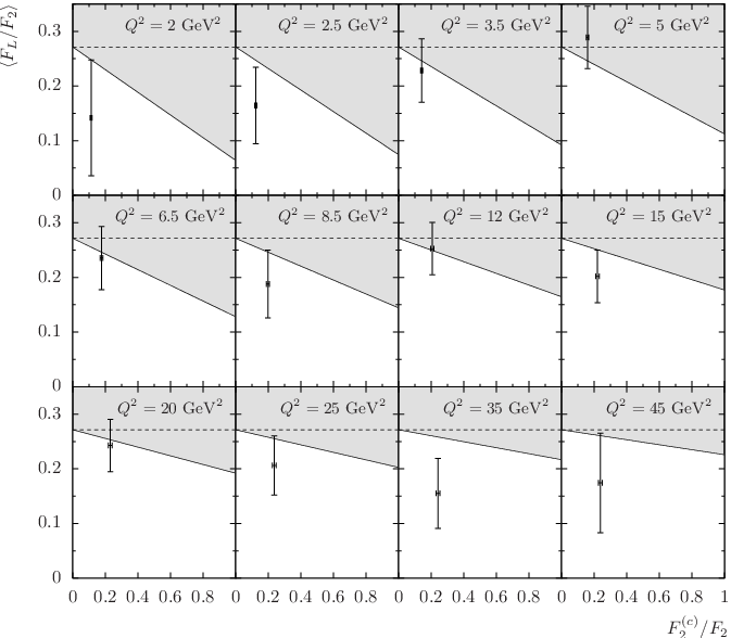
The bounds are calculated for a charm quark mass of $m_{c}=1.23$ GeV. For each data point the corresponding ratio $F_{2}^{(c)}/F_{2}$ is obtained using NLO QCD calculations provided by the OPENQCDRAD package [33], again with a charm pole mass of $m_{c}=1.23$ GeV. For this calculation the JR09FFNNLO parametrisation [34] of the proton parton density functions was used, which was found to describe preliminary HERA charm data [35] very well within the experimental correlated uncertainties of typically 3-9%. Here and in the following we do not consider the data point at $Q^{2}=1.5\,\mbox{GeV}^{2}$ from [1] as it has an exceedingly large error.

The significance of the data points in relation to the bound can be seen more clearly from the quantity

$$\frac{\langle F_{L}/F_{2}\rangle}{\left.(F_{L}/F_{2})\right|_{\rm bound}}$$

(21)

which we plot in figure 4. For this figure the bound $\left.(F_{L}/F_{2})\right|_{\rm bound}$ for each data point is extracted from figure 3 taking into account the corresponding value of $F_{2}^{(c)}/F_{2}$ at that kinematical point.

We see from figures 2-4 that the data for $\langle F_{L}/F_{2}\rangle$ as derived from [1] come very close to the bounds which result from the dipole picture. We now discuss the meaning of this observation from the points of view of both, a dipole-model enthusiast, and a dipole-model sceptic, respectively.

In this paper we have compared the recent data on $F_{L}/F_{2}$ – to be precise: their fixed-$Q^{2}$ averages – with rigorous bounds derived in the framework of the dipole model. Within the experimental errors the bounds are satisfied. But the data is surprisingly close to the bounds for $3.5\,\mbox{GeV}^{2}\leq Q^{2}\leq 20\,\mbox{GeV}^{2}$. We have discussed the meaning of these findings from the points of view of both, the dipole-model enthusiast and the sceptic. The enthusiast will have to admit that the sceptic’s arguments could give problems to the dipole picture if the central values of the data are confirmed with small errors by further experiments. The sceptic will have to concede that, given the errors of the data, $\delta$ functions for the cross sections $\hat{\sigma}^{(q)}(r,\xi)$ as in (25) and (27) are not really necessary and that the widths of the distributions compatible with the data have to be explored. Thus, given the present data, we must leave it to the reader if he will join the camp of the enthusiast or that of the sceptic. More data with small errors would be needed to decide the issue. In any case we hope to have demonstrated in our paper that measurements of $F_{L}/F_{2}$ give very valuable information on the dipole picture, its validity, and potentially on questions like colour transparency and saturation of the dipole-proton cross section. Thus, programs for future electron- and positron-proton scattering experiments (see for instance [36], [37]) certainly should foresee $F_{L}$ measurements as an important item on the list of physics topics.

We are grateful to Sascha Glazov for providing data tables and information on correlated data uncertainties. We would like to thank Markus Diehl for useful discussions. The work of C. E. was supported by the Alliance Program of the Helmholtz Association (HA216/EMMI). The work of A. v. M. was supported by the Schweizer Nationalfonds (Grant 200020_124773/1).

References

- [1] F. D. Aaron et al., Eur. Phys. J. C 71 (2011) 1579 [arXiv:1012.4355 [hep-ex]].
- [2] O. Nachtmann, Elementary Particle Physics: Concepts and Phenomena, Springer Verlag, Berlin, Heidelberg, 1990.
- [3] L. N. Hand, Phys. Rev. 129 (1963) 1834.
- [4] N. N. Nikolaev and B. G. Zakharov, Z. Phys. C 49 (1991) 607.
- [5] N. N. Nikolaev and B. G. Zakharov, Z. Phys. C 53 (1992) 331.
- [6] A. H. Mueller, Nucl. Phys. B 415 (1994) 373.
- [7] K. Golec-Biernat and M. Wüsthoff, Phys. Rev. D 59 (1999) 014017 [arXiv:hep-ph/9807513].
- [8] K. Golec-Biernat and M. Wüsthoff, Phys. Rev. D 60 (1999) 114023 [arXiv:hep-ph/9903358].
- [9] J. Bartels, K. Golec-Biernat and H. Kowalski, Phys. Rev. D 66 (2002) 014001 [arXiv:hep-ph/0203258].
- [10] M. McDermott, L. Frankfurt, V. Guzey and M. Strikman, Eur. Phys. J. C 16 (2000) 641 [arXiv:hep-ph/9912547].
- [11] H. G. Dosch, T. Gousset and H. J. Pirner, Phys. Rev. D 57 (1998) 1666 [arXiv:hep-ph/9707264].
- [12] A. Donnachie and H. G. Dosch, Phys. Rev. D 65 (2002) 014019 [arXiv:hep-ph/0106169].
- [13] A. I. Shoshi, F. D. Steffen and H. J. Pirner, Nucl. Phys. A 709 (2002) 131 [arXiv:hep-ph/0202012].
- [14] E. Iancu, K. Itakura and S. Munier, Phys. Lett. B 590 (2004) 199 [arXiv:hep-ph/0310338].
- [15] J. R. Forshaw, G. Kerley and G. Shaw, Phys. Rev. D 60 (1999) 074012 [arXiv:hep-ph/9903341].
- [16] J. R. Forshaw and G. Shaw, JHEP 0412 (2004) 052 [arXiv:hep-ph/0411337].
- [17] J. R. Forshaw, R. Sandapen and G. Shaw, JHEP 0611 (2006) 025 [arXiv:hep-ph/0608161].
- [18] H. Kowalski and D. Teaney, Phys. Rev. D 68 (2003) 114005 [arXiv:hep-ph/0304189].
- [19] G. Watt and H. Kowalski, Phys. Rev. D 78 (2008) 014016 [arXiv:0712.2670 [hep-ph]].
- [20] L. Motyka, K. Golec-Biernat and G. Watt, in Proceedings of HERA and the LHC: 4th Workshop on the Implications of HERA for LHC Physics, Geneva, May 2008, p. 471 [arXiv:0809.4191 [hep-ph]].
- [21] G. Cvetic, D. Schildknecht, B. Surrow and M. Tentyukov, Eur. Phys. J. C 20 (2001) 77 [arXiv:hep-ph/0102229].
- [22] D. Schildknecht, B. Surrow and M. Tentyukov, Phys. Lett. B 499 (2001) 116 [arXiv:hep-ph/0010030].
- [23] M. Kuroda and D. Schildknecht, Phys. Lett. B 618 (2005) 84 [arXiv:hep-ph/0503251].
- [24] M. Kuroda and D. Schildknecht, Phys. Lett. B 670 (2008) 129 [arXiv:0806.0202 [hep-ph]].
- [25] D. Schildknecht, arXiv:1104.0850 [hep-ph].
- [26] M. Kuroda and D. Schildknecht, arXiv:1108.2584 [hep-ph].
- [27] J. L. Albacete, N. Armesto, J. G. Milhano and C. A. Salgado, Phys. Rev. D 80 (2009) 034031 [arXiv:0902.1112 [hep-ph]].
- [28] C. Ewerz and O. Nachtmann, Annals Phys. 322 (2007) 1635 [arXiv:hep-ph/0404254].
- [29] C. Ewerz and O. Nachtmann, Annals Phys. 322 (2007) 1670 [arXiv:hep-ph/0604087].
- [30] C. Ewerz and O. Nachtmann, Phys. Lett. B 648 (2007) 279 [arXiv:hep-ph/0611076].
- [31] C. Ewerz, A. von Manteuffel and O. Nachtmann, Phys. Rev. D 77 (2008) 074022 [arXiv:0708.3455 [hep-ph]].
- [32] C. Ewerz, A. von Manteuffel and O. Nachtmann, JHEP 1103 (2011) 062 [arXiv:1101.0288 [hep-ph]].
- [33] A. Alekhin, J. Blümlein and S. Moch, OPENQCDRAD package, version 1.4 http://www-zeuthen.desy.de/alekhin/OPENQCDRAD/
- [34] P. Jimenez-Delgado and E. Reya, Phys. Rev. D 79 (2009) 074023 [arXiv:0810.4274 [hep-ph]].
- [35] M. Corradi for the H1 and ZEUS Collaborations, in Proceedings of 35th International Conference on High Energy Physics ICHEP 2010, Paris, July 2010, PoS ICHEP2010 (2010) 142.
- [36] C. Aidala et al., The EIC Working Group, A high luminosity, high energy electron-ion-collider - A white paper prepared for the NSAC LRP 2007, http://web.mit.edu/eicc/DOCUMENTS/EIC_LRP-20070424.pdf
- [37] M. Klein for the LHeC Study Group, in Proceedings of 35th International Conference on High Energy Physics ICHEP 2010, Paris, July 2010, PoS ICHEP2010 (2010) 520.