On range and local time of many-dimensional submartingales

Let ${\mathfrak{X}}\subset{\mathbb{R}}^{d}$ be a set of infinite cardinality; the elements of ${\mathfrak{X}}$ will be called sites. Without restriction of generality, we assume that $0\in{\mathfrak{X}}$. Throughout this paper we assume that $d\geq 2$. We consider a discrete-time process $X=(X_{n},n\geq 0)$ with values in ${\mathfrak{X}}$, adapted to a filtration $\mathcal{F}=(\mathcal{F}_{n},n\geq 0)$. For the process $X$, we suppose that it is uniformly elliptic (can advance in any given direction with uniformly positive probability), has uniformly bounded jumps, and is a strongly directed submartingale (see Definition 1.1 below for the precise meaning). In principle, we do not assume homogeneity in space and/or time, or even the fact that the process is Markovian.

In this paper we study two related questions:

• •

  How many different sites can be visited by the process $X$ by time $n$?

• •

  How large can be the number of visits to a given site?

Of course, in the absence of space/time homogeneity one cannot hope to be able to characterize the precise behavior of the quantities of interest; in this paper we content ourselves in proving that with probability $1-\exp(-n^{\varepsilon})$ the number of visits to any fixed site by time $n$ is less than $n^{\frac{1}{2}-\delta}$ for some $\delta>0$. This in its turn implies that the number is different sites visited by the process by time $n$ with very high probability will be at least $n^{\frac{1}{2}+\delta}$.

Although it is not important for the formulation of our results, while reading the paper one may always assume that ${\mathfrak{X}}$ is the vertex set of the integer lattice ${\mathbb{Z}}^{d}$, the vertex set of some other mosaic, or just any “discrete” (in particular, countable) set. This, of course, is justified by the questions that are of our interest: e.g., if the law of the jump of the process is (in some sense) continuous, then such questions typically do not arise (every site is visited at most once, and the process visits $n$ different sites by time $n$).

Range (i.e., the cardinality of the set visited sites, or sometimes this set itself) and the local time (i.e., the number of visits to a given site) for space-homogeneous discrete-time random walks were extensively studied in the literature. It is a classical result that the expected range of the simple random walk is $O(\frac{n}{\ln n})$ for $d=2$ and $O(n)$ for $d\geq 3$, see e.g. Section 6.1 of [13]. It is not difficult to obtain from this fact (using an independence argument as e.g. in Lemma 3.1 of [1]) that with very high probability the walk visits at least $n^{1-\delta}$ distinct sites by time $n$. Finer results for the range of homogeneous random walks can be found in a number of papers; see e.g. in [3, 10, 11] and references therein. For nonhomogeneous random walks these questions, of course, are more difficult; we mention [17] that contains results on the range of simple random walk on supercritical percolation cluster.

The behaviour of the local time (i.e., the number of visits) in a fixed site, or the field of local times in all sites, was much studied in the literature as well. It is quite elementary to obtain that the expected number of visits to the origin by time $n$ for the simple random walk is $O(\ln n)$ for $d=2$ and $O(1)$ for $d\geq 3$. Also, one can easily obtain for the simple random walk in dimension $2$ (using e.g. E1 of Section III.16 of [18]) that, with stretched-exponentially small probability, the number of visits to the origin is less than $n^{\delta}$ for any fixed $\delta>0$. Of course, finer results (for more general random walks as well) are available; see e.g. [6, 7, 8, 9, 15].

As mentioned above, with our assumptions we cannot hope to obtain very “precise” results; however, in some cases it may be important to be able to estimate the range from below. In particular, consider the following process, called excited random walk, or sometimes cookie random walk. It is a discrete-time stochastic process taking values on ${\mathbb{Z}}^{d}$, $d\geq 2$, described in the following way: when the particle visits a site for the first time, it has a uniformly positive drift in a given direction $\ell$; when the particle is at a site which was already visited before, it has zero drift (observe that this implies that the cookie random walk is a strongly directed submartingale in the sense of Definition 1.1 below). This process was introduced in a simpler form ($\ell$ is the first coordinate vector and in already visited sites the process behaves as simple random walk) in [4] and then studied (we mention only the papers that are concerned with dimension $d\geq 2$) in e.g. [5, 12, 16, 19]. The key fact that is usually needed is that such a process typically visits much more than $n^{1/2}$ different sites by time $n$; this allows to prove bounds on the probability that the process advances in the direction of cookies’ drift by much more than $Cn^{1/2}$, and this in turn makes is possible to use regeneration arguments that imply the Law of Large Numbers and the Central Limit Theorem.

It is worth noting that in this paper, differently from what was considered in [16], we allow the process to have a nonzero drift of arbitrarily small absolute value; for such processes, a direct application of methods of [16] fails.

Now, we write formal definitions and state our results. Let $\|\cdot\|$ be the Euclidean norm in ${\mathbb{R}}^{d}$ and let $\mathbb{S}^{d-1}=\{x\in{\mathbb{R}}^{d}:\|x\|=1\}$ be the unit sphere. Let us denote the coordinate vectors of ${\mathbb{R}}^{d}$ by $\mathbf{e}_{1},\ldots,\mathbf{e}_{d}$. We write $x\cdot y$ for the usual scalar product of $x,y\in{\mathbb{R}}^{d}$. For $A\subset{\mathfrak{X}}$ we denote by $|A|$ the cardinality of $A$. Let

$$L_{n}(x)=\sum_{k=0}^{n}{\mathbf{1}}_{\{X_{k}=x\}}$$

(1.1)

be the local time of the process in $x\in{\mathfrak{X}}$ by time $n$, and we denote by ${\mathcal{R}}_{n}=\{X_{0},\ldots,X_{n}\}$ the set of visited sites by time $n$. Define the random variable $D_{n}\in{\mathbb{R}}^{d}$ to be the (conditional) drift of the process $X$ at time $n$:

$$D_{n}=\mathbb{E}(X_{n+1}-X_{n}\mid\mathcal{F}_{n})=\mathbb{E}(X_{n+1}\mid\mathcal{F}_{n})-X_{n}.$$

Next, let ${\mathcal{P}}_{\mathcal{L}}$ be the operator of projection on the linear subspace ${\mathcal{L}}\subset{\mathbb{R}}^{d}$. Assuming that ${\mathcal{L}}$ is a two-dimensional subspace of ${\mathbb{R}}^{d}$, $\ell\in\mathbb{S}^{d-1}\cap{\mathcal{L}}$ and $u\in{\mathbb{R}}$, define

$$H_{\ell,{\mathcal{L}}}^{u}=\Big\{x\in{\mathbb{R}}^{d}:{\mathcal{P}}_{\mathcal{L}}x=0\text{ or }\frac{{\mathcal{P}}_{\mathcal{L}}x\cdot\ell}{\|{\mathcal{P}}_{\mathcal{L}}x\|}\geq u\Big\},$$

see Figure 1.

Observe that for $(u,\ell,{\mathcal{L}})$-strongly directed submartingale it holds that the (conditional on the history) expected projection of the drift to $\ell$ is always nonnegative (so that it is what one would naturally call a “submartingale in direction $\ell$”).

In this paper we assume that all processes we are considering live in a probability space with probability measure $\mathbb{P}$. We also adopt the following notational convention: when it is necessary to assume that the initial state of the process under consideration is $x\in{\mathfrak{X}}$, we do not write it explicitly but simply add a subscript $x$ to $\mathbb{P}$.

It is known that for the many-dimensional uniformly elliptic martingales with bounded jumps the following result (well hidden in [16] as Lemma 5.3 and a part of argument in Lemma 5.4) holds:

One can note (we discuss this in detail in Section 3) that (1.3) follows from (1.2) in an elementary way.

The main purpose of this paper is to generalize Theorem 1.2 to (strongly directed) submartingales. Observe that one really needs some additional condition on the submartingale; otherwise it may happen that the typical number of visited sites is of order $n^{1/2}$. Indeed, consider the following example:

The main result of this paper is the following

The key to the proof of Theorem 1.4 is a technical fact about exit probabilities from two-dimensional rectangular domains for martingales. For a simply connected domain ${\mathcal{D}}\subset{\mathbb{R}}^{2}$, denote by

$$\tau({\mathcal{D}})=\min\{k\geq 1:X_{k}\notin{\mathcal{D}}\}$$

the exit time from the domain ${\mathcal{D}}$. Let

$$\mathcal{S}({\mathcal{D}})=\{\alpha X_{\tau({\mathcal{D}})-1}+(1-\alpha)X_{\tau({\mathcal{D}})},0\leq\alpha\leq 1\}\subset{\mathbb{R}}^{2}$$

be the segment of the trajectory of the process at the instant when it leaves ${\mathcal{D}}$.

For $v\in\mathbb{S}^{1}$ and $a,b,c,\lambda>0$, let us define a rectangular domain

$$R_{v,\lambda}^{a,b,c}(x)=\big\{y\in{\mathbb{R}}^{2}:|(y-x)\cdot v^{\bot}|<a\lambda,(y-x)\cdot v\in(-b\lambda,c\lambda)\big\},$$

where $v^{\bot}$ is a unit vector perpendicular to $v$, and consider the event

$$G_{v,\lambda}^{a,b,c}(x)=\Big\{\mathcal{S}(R_{v,\lambda}^{a,b,c}(x))\cap\{y\in{\mathbb{R}}^{2}:|(y-x)\cdot v^{\bot}|\leq a\lambda,(y-x)\cdot v=-b\lambda\}\neq\emptyset\Big\}$$

which means the process goes out of the rectangle through its “left” side, see Figure 2.

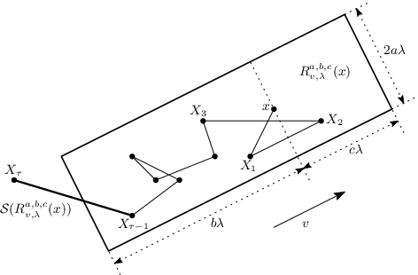
Now, the important technical fact in the proof of Theorem 1.4 is

The explicit expressions for $\varrho(a,b,c)$ and $\lambda_{0}(a,b,c)$ can be found at the end of the proof of Theorem 1.5, see (2.11) and (2.12).

In fact, there is only a small distance from the last result to a more general one: let ${\mathcal{D}}$ be a “nice” domain such that $0\in{\mathcal{D}}$, and suppose that $A\subset\partial{\mathcal{D}}$ is a connected piece of the boundary of ${\mathcal{D}}$ with positive measure. Then there exist $\varrho=\varrho({\mathcal{D}},A)>0$ and $\lambda_{0}=\lambda_{0}({\mathcal{D}},A)$ such that $\mathbb{P}_{x}[\mathcal{S}(x+\lambda{\mathcal{D}})\cap(x+\lambda A)\neq\emptyset]\geq\varrho$ for all $\lambda\geq\lambda_{0}$ and all $x\in{\mathfrak{X}}$. It is not our intention in this paper to investigate, under which (not very restrictive) precise geometric assumptions on ${\mathcal{D}}$ and $A$ the above fact holds; the way how it should follow from Theorem 1.5 is (hopefully) made clear by Figure 3.

The paper is organized in the following way. In Section 2 we prove Theorem 1.5. Then, in Section 3 we prove the main result of this paper, Theorem 1.4. In Section 4, for comparison purposes we give a sketch of the proof of Theorem 1.2, and then discuss some open problems.

We begin with the following lemma.

It is easy to believe that this result should hold true: it essentially means that if the rectangle is (relatively) thin enough, then with uniformly positive probability the process will exit the rectangle through a fixed long side (in this case, the “left” one), see Figure 4. In fact, the constant $1/7$ was chosen just for definiteness: one can modify the assumptions to obtain any fixed number less than $1/2$ on its place.

Next, since $X_{\cdot\wedge\tau_{1}}\cdot\mathbf{e}_{1}$ is a (one-dimensional) bounded martingale, using the Optional Stopping Theorem we write

	$\displaystyle 0$	$\displaystyle=\mathbb{P}_{0}[\tau_{\leftarrow}<\tau_{\to}]\mathbb{E}_{0}(X_{\tau_{1}}\cdot\mathbf{e}_{1}\mid\tau_{\leftarrow}<\tau_{\to})+\mathbb{P}_{0}[\tau_{\leftarrow}>\tau_{\to}]\mathbb{E}_{0}(X_{\tau_{1}}\cdot\mathbf{e}_{1}\mid\tau_{\leftarrow}>\tau_{\to})$
		$\displaystyle\geq-(b\lambda+K)\mathbb{P}_{0}[\tau_{\leftarrow}<\tau_{\to}]+b\lambda(1-\mathbb{P}_{0}[\tau_{\leftarrow}<\tau_{\to}])$
		$\displaystyle=b\lambda-(2b\lambda+K)\mathbb{P}_{0}[\tau_{\leftarrow}<\tau_{\to}],$

so

$$\mathbb{P}_{0}[\tau_{\leftarrow}<\tau_{\to}]\geq\frac{b\lambda}{2b\lambda+K}>\frac{3}{7}$$

(2.3)

since $\lambda>\frac{3K}{b}$.

Then, observe that Doob’s inequality together with the fact that the jumps are bounded by $K$ imply that (abbreviate $s_{\lambda}:=\frac{7(b\lambda+K)^{2}}{r^{2}h}$)

	$\displaystyle\mathbb{P}_{0}\Big[\max_{j\leq s_{\lambda}}|X_{j}\cdot\mathbf{e}_{2}|\geq a\lambda\Big]$	$\displaystyle\leq\frac{\mathbb{E}_{0}(X_{\lfloor s_{\lambda}\rfloor}\cdot\mathbf{e}_{2})^{2}}{a^{2}\lambda^{2}}$
		$\displaystyle\leq\frac{K^{2}s_{\lambda}}{a^{2}\lambda^{2}}$
		$\displaystyle\leq\frac{7K^{2}(b+K)^{2}}{r^{2}ha^{2}}\leq\frac{1}{7},$		(2.4)

recall that we assumed that $a\geq\frac{7K(b+K)}{r\sqrt{h}}$. The claim of Lemma 2.1 now follows from (2.2), (2.3), and (2.4). $\Box$

Now, we are ready to prove Theorem 1.5.

Now, we define inductively two sequences of stopping times: $\sigma(0)=T(0)=0$, and

	$\displaystyle\sigma(m+1)$	$\displaystyle=\min\big\{k>\sigma(m):\theta(X_{\sigma(m)},X_{k})\in[\alpha_{0},\pi)\big\}$
	$\displaystyle T(m+1)$	$\displaystyle=\min\Big\{k>\sigma(m):X_{k}\cdot\frac{X_{\sigma(m)}}{\|X_{\sigma(m)}\|}\notin\Big[\frac{\|X_{\sigma(m)}\|}{2},\frac{3\|X_{\sigma(m)}\|}{2}\Big]\Big\},$

for $m\geq 1$.

Define the sequence of events $A_{k}=\{\sigma(k)<T(k)\}$, $k\geq 1$. Lemma 2.1 then implies (see Figure 5 and recall that this lemma holds for rectangles with smaller side at least $3K$) that

	$\displaystyle\mathbb{P}\big[A_{k+1}\mid\mathcal{F}_{\sigma(k)},\|X_{\sigma(k)}\|\geq 6Ka_{0}\big]$	$\displaystyle\geq\mathbb{P}\big[G^{a_{0},1,1}_{v_{k},\lambda_{k}}(X_{\sigma(k)})\mid\mathcal{F}_{\sigma(k)},\|X_{\sigma(k)}\|\geq 6Ka_{0}\big]$
		$\displaystyle\geq\frac{1}{7},$		(2.9)

where $v_{k}=\big(\frac{X_{\sigma(k)}}{\|X_{\sigma(k)}\|}\big)^{\bot}$, $\lambda_{k}=\frac{\|X_{\sigma(k)}\|}{2a_{0}}$.

Now, let us define

$${\hat{\sigma}}=\min\{k\geq 1:X_{k}\cdot\mathbf{e}_{1}<0,0\leq X_{k}\cdot\mathbf{e}_{2}<K\},$$

and abbreviate as ${\mathcal{P}}_{1}$ the projector on the linear subspace spanned by $\mathbf{e}_{1}$. Then, (2.9) implies (see Figure 6) that for any $x_{0}$ such that $\|x_{0}\|\geq s_{0}$ (recall (2.8)), $x_{0}\cdot\mathbf{e}_{1}>0$, $|x_{0}\cdot\mathbf{e}_{2}|\leq K$ we have

$$\mathbb{P}_{x_{0}}\Big[X_{{\hat{\sigma}}}\cdot\mathbf{e}_{1}\in[-2^{m_{0}}\|x_{0}\|,-2^{-m_{0}}\|x_{0}\|],\;\max_{k\leq{\hat{\sigma}}}\|X_{k}-{\mathcal{P}}_{1}x_{0}\|<2^{m_{0}}\|x_{0}\|\Big]\geq\frac{1}{7^{m_{0}}}.$$

(2.10)

Now, we finish the proof of Theorem 1.5. Again, without lost of generality we assume that $x=0$ and $v=\mathbf{e}_{1}$. Also, let us assume that $\lambda 2^{-m_{0}}(a\wedge c)>s_{0}$.

For $n\geq 1$, let us define the sequence of stopping times, starting with $\tau_{0}=0$, by

	$\displaystyle\tau_{n}$	$\displaystyle=\min\Big\{t\geq\tau_{n}:(X_{t}-X_{\tau_{n-1}})\cdot\mathbf{e}_{1}<-\lambda 2^{-m_{0}}(a\wedge c),$
		$\displaystyle\qquad\qquad\qquad X_{t}\cdot\mathbf{e}_{2}\in[0,K],\max_{k\in[\tau_{n-1},t]}\|X_{k}-{\mathcal{P}}_{1}X_{\tau_{n-1}}\|<\lambda(a\wedge c)\Big\}$

(we set formally $\min\emptyset=+\infty$), and define the events $M_{n}=\{\tau_{n}<\infty\}$. From (2.10) we obtain that $\mathbb{P}[M_{n}\mid\mathcal{F}_{\tau_{n-1}}]\geq 7^{-m_{0}}$, and, clearly, it holds that

$$G^{a,b,c}_{\mathbf{e}_{1},\lambda}(0)\supset\bigcup_{n=1}^{\lceil\frac{2^{m_{0}}b}{a\wedge c}\rceil}M_{n}$$

(since on each of the events $M_{n}$ the process advances to the left by at least $\lambda 2^{-m_{0}}(a\wedge c)$, while staying inside the rectangle $R^{a,b,c}_{\mathbf{e}_{1},\lambda}(0)$). This concludes the proof of Theorem 1.5; the explicit expressions for $\varrho$ and $\lambda_{0}$ are then given by

	$\displaystyle\lambda_{0}$	$\displaystyle=\frac{s_{0}}{a\wedge c}$		(2.11)
and
	$\displaystyle\varrho$	$\displaystyle=\exp\Big(-m_{0}\Big\lceil\frac{2^{m_{0}}b}{a\wedge c}\Big\rceil\ln 7\Big),$		(2.12)

with $m_{0},s_{0}$ defined by (2.5)–(2.8). $\Box$

We consider first the case $d=2$. For this case, abbreviate $H^{u}_{\ell}:=H^{u}_{\ell,{\mathbb{R}}^{2}}$. Define $Y_{0}=X_{0}$,

$$Y_{n}=X_{n}-\sum_{k=0}^{n-1}D_{k}$$

for $n\geq 1$. Clearly, $Y$ is a martingale with jumps uniformly bounded by $K^{\prime}=2K$. To prove that $Y$ is uniformly elliptic, let us define

$$\tilde{D}_{n}=\begin{cases}\frac{D_{n}}{\|D_{n}\|},&\text{ on }\{D_{n}\neq 0\},\\ \mathbf{e}_{1},&\text{ on }\{D_{n}=0\}.\end{cases}$$

Then, observe that $Y_{n+1}-Y_{n}=X_{n+1}-X_{n}-D_{n}$, so we have

$$\mathbb{P}[(Y_{n+1}-Y_{n})\cdot Z\geq r\mid\mathcal{F}_{n}]=\mathbb{P}[(X_{n+1}-X_{n})\cdot Z\geq r\mid\mathcal{F}_{n}]\geq h$$

(3.1)

for $Z\in\{\tilde{D}_{n}^{\bot},-\tilde{D}_{n}^{\bot}\}$, and

$$\mathbb{P}[(Y_{n+1}-Y_{n})\cdot(-\tilde{D}_{n})\geq r\mid\mathcal{F}_{n}]\geq\mathbb{P}[(X_{n+1}-X_{n})\cdot(-\tilde{D}_{n})\geq r\mid\mathcal{F}_{n}]\geq h.$$

(3.2)

Using that $Y$ is a martingale and $\tilde{D}_{n}$ is $\mathcal{F}_{n}$-measurable, we have $\mathbb{E}\big((Y_{n+1}-Y_{n})\cdot\tilde{D}_{n}\mid\mathcal{F}_{n}\big)=0$. Since (3.2) implies that $\mathbb{E}\big((Y_{n+1}-Y_{n})\cdot\tilde{D}_{n}\mid\mathcal{F}_{n}\big)^{-}=\mathbb{E}\big((Y_{n+1}-Y_{n})\cdot\tilde{D}_{n}\mid\mathcal{F}_{n}\big)^{+}\geq rh$ and we have also $\big((Y_{n+1}-Y_{n})\cdot\tilde{D}_{n}\big)^{+}\leq 2K$, it holds that¹¹ 1 it is elementary to obtain that for any random variable $\xi$ with $0\leq\xi\leq a$ a.s. and $\mathbb{E}\xi\geq b$, it is true that $\mathbb{P}[\xi\geq b/2]\geq b/(2a)$

$$\mathbb{P}[(Y_{n+1}-Y_{n})\cdot\tilde{D}_{n}\geq rh/2]\geq\frac{rh}{4K}.$$

(3.3)

Then, (3.1)–(3.3) imply that the process $Y$ is uniformly elliptic with $r^{\prime}=\frac{rh}{2\sqrt{2}}$ and $h^{\prime}=\frac{rh}{4K}$ (recall that we assume without restricting generality that $K\geq 1$).

Next, let us define

	$\displaystyle{\tilde{\sigma}}$	$\displaystyle=\min\{j\geq 1:Y_{j}\in H_{-\ell}^{u}\},$
	$\displaystyle\sigma_{0}$	$\displaystyle=\min\{j\geq 1:Y_{j}\cdot\ell\leq 0\},$

and, for $k\geq 1$

$$\sigma_{k}=\min\{j\geq 1:Y_{j}\cdot\ell\geq k\}.$$

Now, our goal is to find a lower bound on the probability that, starting from $0\in{\mathfrak{X}}$, the process avoids the origin for the next $k$ steps. Clearly, since $X_{k}-Y_{k}\in H_{\ell}^{u}$ a.s., for any $k$ it holds that

$$\mathbb{P}_{0}[Y_{1}\notin H_{-\ell}^{u},\ldots,Y_{k}\notin H_{-\ell}^{u}]\leq\mathbb{P}_{0}[X_{1}\neq 0,\ldots,X_{k}\neq 0],$$

(3.4)

so we concentrate on finding a lower bound for the term in the left-hand side of the above display.

For that, let us prove that there exists $\beta>\frac{1}{2}$ and $m_{1}$ such that for all $m\geq m_{1}$

$$\mathbb{P}_{y}[\sigma_{2m}<{\tilde{\sigma}}]\geq\beta$$

(3.5)

for all $y\in{\mathfrak{X}}$ such that $y\cdot\ell\in[m,m+K)$. First, note that the Optional Stopping Theorem implies analogously to (2.3) that

$$\mathbb{P}_{y}[\sigma_{2m}<\sigma_{0}]\geq\frac{m}{2m+K}$$

(3.6)

for all $y$ such that $y\cdot\ell\in[m,m+K)$.

Abbreviate $W_{0}^{\ell}=\{x\in{\mathbb{R}}^{2}:x\cdot\ell\in(-K,0]\}$ and consider two vectors $v_{1},v_{2}\in\mathbb{S}^{1}$ such that $v_{j}\cdot\ell>0$ for $j=1,2$ and $v_{1}+v_{2}$ is collinear to $\ell$. Then, there exist $a_{1},b_{1},c_{1},a_{2},b_{2},c_{2}>0$ such that

• (i)

  we have

  	$\displaystyle b_{1}|\cos\theta(v_{1},\ell)|-a_{1}|\sin\theta(v_{1},\ell)|$	$\displaystyle>1,$
  	$\displaystyle a_{1}|\sin\theta(v_{1},\ell)|+c_{1}|\cos\theta(v_{1},\ell)|$	$\displaystyle<1$

• (ii)

  $b_{2}>1$,

• (iii)

  for $j=1,2$ the set

  $$R^{a_{1},b_{1},c_{1}}_{v_{j},m}(m\ell)\cup\bigcup_{y\in W_{0}\cap R^{a_{1},b_{1},c_{1}}_{v_{j},m}(m\ell)}R^{a_{2},b_{2},c_{2}}_{-\ell,m}(y)$$

  does not intersect $H_{-\ell}^{u}$,

see Figure 7.

In words, (i) means that (for large enough $m$) the left side of the inclined rectangles lies to the left of the dotted line (level $0$) and the right side does not reach the level $2m$, (ii) means that the right side of the horizontal rectangle (relative to a point close to where the inclined rectangle intersect with the dotted line) is to the right of the level $m$, and (iii) means that the two rectangles cannot touch the set $H_{-\ell}^{u}$. Then, it is clear that Theorem 1.5 and (3.6) imply that there exist $m_{1},\varepsilon>0$ such that for all $m\geq m_{1}$

$$\mathbb{P}_{y}[\sigma_{0}<\sigma_{2m},\sigma_{2m}<{\tilde{\sigma}}]\geq\varepsilon$$

(3.7)

for any $y$ such that $y\cdot\ell\in[m,m+K)$. Since

$$\mathbb{P}_{y}[\sigma_{2m}<{\tilde{\sigma}}]=\mathbb{P}_{y}[\sigma_{2m}<\sigma_{0}]+\mathbb{P}_{y}[\sigma_{0}<\sigma_{2m},\sigma_{2m}<{\tilde{\sigma}}],$$

we obtain (3.5) from (3.6) and (3.7).

Next, denote

$$k_{1}=\Big\lceil\log_{2}\frac{K\sqrt{2n}}{m_{1}}\Big\rceil;$$

observe that $m_{1}2^{k_{1}}\geq K\sqrt{2n}$. Analogously to (2.4), applying Doob’s inequality we obtain that

$$\mathbb{P}_{y}[\sigma_{0}>n]\geq\frac{1}{2}$$

(3.8)

for all $y$ such that $y\cdot\ell\geq K\sqrt{2n}$. Then, (3.5) implies that for any $y$ such that $y\cdot\ell\geq m_{1}$

$$\mathbb{P}_{y}[\sigma_{K\sqrt{2n}}<{\tilde{\sigma}}]\geq\beta^{k_{1}}.$$

(3.9)

So, using (3.8)–(3.9) and uniform ellipticity (to assure that the process can initially advance to level $m_{1}$), we obtain for some ${\tilde{c}}>0$, $\varepsilon>0$,

$$\mathbb{P}_{0}[Y_{1}\notin H_{-\ell}^{u},\ldots,Y_{n}\notin H_{-\ell}^{u}]=\mathbb{P}_{0}[{\tilde{\sigma}}>n]\geq\frac{(h^{\prime})^{\lceil m_{1}/r^{\prime}\rceil}}{2}\beta^{k_{1}}\geq{\tilde{c}}n^{-\frac{1}{2}+\varepsilon}$$

(3.10)

since $\beta>\frac{1}{2}$. Using (3.4), we obtain (1.4) for $d=2$; for $d\geq 3$ it then follows if one considers the projection on ${\mathcal{L}}$.

To prove (1.5), define ${\hat{\tau}}_{0}=0$,

$${\hat{\tau}}_{k+1}=\min\big\{m>{\hat{\tau}}_{k}:X_{m}\notin\{X_{0},\ldots,X_{m-1}\}\big\};$$

i.e., $({\hat{\tau}}_{k},k\geq 0)$ is the sequence of times when the process enters previously unvisited sites. Then, to obtain (1.5), we use the fact that the process $X^{(k)}_{\cdot}=X_{\cdot+{\hat{\tau}}_{k}}$ satisfies conditions of the theorem, and apply the union bound (again, the projection argument implies that (1.5) holds for all $d\geq 2$). This concludes the proof of Theorem 1.4. $\Box$

First, let us briefly sketch the proof of Theorem 1.2. So, suppose that $X$ is a martingale in dimension $d\geq 2$, with bounded jumps and uniform ellipticity. To begin, we show that there exist $b\in(0,1)$ close enough to $1$ and $\gamma^{\prime}>0$ (depending only on $K$, $h$, $r$ — the constants in Definition 1.1 (a)–(b)) such that

$$\mathbb{E}(\|X_{n+1}\|^{b}\mid\mathcal{F}_{n})\geq\|X_{n}\|^{b}{\mathbf{1}}_{\{\|Y_{n}\|>\gamma^{\prime}\}}.$$

(4.1)

To see that (4.1) holds, first observe that for a fixed $y\in{\mathbb{R}}^{d}$ we have

	$\displaystyle\|x+y\|^{b}$	$\displaystyle=\big(\|x\|^{2}+2x\cdot y+\|y\|^{2}\big)^{b/2}$
		$\displaystyle=\|x\|^{b}\Big(1+b\frac{x\cdot y}{\|x\|^{2}}+\frac{b\|y\|^{2}}{2\|x\|^{2}}-\frac{1}{2}b(2-b)\frac{(x\cdot y)^{2}}{\|x\|^{4}}+o(\|x\|^{-2})\Big),$		(4.2)

as $x\to\infty$. So, denoting by $\varphi_{n}$ the angle between $x$ and $\Delta_{n}:=X_{n+1}-x$, we have

	$\displaystyle\mathbb{E}(\|X_{n+1}\|^{b}-\|X_{n}\|^{b}\mid\mathcal{F}_{n},X_{n}=x)$
		$\displaystyle=\frac{b}{2\|x\|^{2-b}}\big(\mathbb{E}(\|\Delta_{n}\|^{2}\mid\mathcal{F}_{n})-(2-b)\mathbb{E}(\|\Delta_{n}\|^{2}\cos^{2}\varphi_{n}\mid\mathcal{F}_{n})+o(\|x\|^{-2})\big).$			(4.3)

Using the uniform ellipticity and the boundedness of jumps, one can obtain that

$$\mathbb{E}(\|\Delta_{n}\|^{2}\cos^{2}\varphi_{n}\mid\mathcal{F}_{n})<(1-\varepsilon^{\prime})\mathbb{E}(\|\Delta_{n}\|^{2}\mid\mathcal{F}_{n})$$

for some $\varepsilon^{\prime}>0$, so if $b<1$ is close enough to $1$, the right-hand side of (4.3) is positive for all large enough $x$ (see more details in the proof of Lemma 5.2 in [16]).

Denote by ${\mathcal{B}}(x,s)=\{y\in{\mathbb{R}}^{d}:\|x-y\|\leq s\}$ the closed ball of radius $s$ centered in $x$. The proof of Theorem 1.2 is now quite straightforward:

• •

  the Optional Stopping Theorem implies that, starting from $x_{0}\in{\mathbb{R}}^{d}$, the process $X$ will reach ${\mathbb{R}}^{d}\setminus{\mathcal{B}}(x_{0},\alpha)$ (without coming back to $0$) with probability at least $O(\alpha^{-b})$ (to apply the Optional Stopping Theorem, one has first to force the process a bit away from the origin, which happens with positive probability by uniform ellipticity).

• •

  Doob’s inequality implies that from any place in ${\mathbb{R}}^{d}\setminus{\mathcal{B}}(x_{0},\alpha)$ with probability bounded away from $0$ the process will not return to $x_{0}$ after additional ${\tilde{c}}_{1}\alpha^{2}$ steps, where ${\tilde{c}}_{1}>0$ is a small enough constant.

• •

  Then, consider $\alpha={\tilde{c}}_{2}n^{1/2}$ for large enough ${\tilde{c}}_{2}$. By the previous discussion, each time the process is in $x_{0}$, independently of the past it has probability at least of order $n^{-b/2}$ of not returning to $x_{0}$ during next $n$ steps.

• •

  Take $\varepsilon>0$ such that $b+\varepsilon<1$. Then, by an obvious coin-tossing argument, the number of visits to $x_{0}$ by time $n$ will not exceed $n^{\frac{b+\varepsilon}{2}}$ with probability at least $1-{\tilde{c}}_{3}e^{-{\tilde{c}}_{4}n^{\varepsilon/2}}$.

• •

  So, with probability at least $1-{\tilde{c}}_{3}ne^{-{\tilde{c}}_{4}n^{\varepsilon/2}}$ the process $X$ will have to visit at least $n^{1-\frac{b+\varepsilon}{2}}$ different sites.

Now, we see that this proof is in sharp contrast with the proof of Theorem 1.4. Originally, our intention was to find a proof for Theorem 1.4 that would use Lyapunov functions in a similar way; this amounts to finding a function $f:{\mathbb{R}}^{2}\mapsto{\mathbb{R}}$ with the following properties: $f\equiv 0$ on $\partial H^{-u}_{\mathbf{e}_{1}}$,

$$\sup_{x\in\partial H^{u}_{\mathbf{e}_{1}}+n^{1/2}\mathbf{e}_{1}}f(x)=O(n^{\frac{1}{2}-\varepsilon})$$

for some $\varepsilon>0$, and $f(X_{\cdot\wedge\tau})$ is a submartingale, where $\tau$ is the hitting time of $H^{u}_{-\mathbf{e}_{1}}$. A possible idea would be to modify somehow the function $f_{w}$ of formula (3.5) of [14], but we did not succeed in developing it properly.

References

- [1] O.S.M. Alves, F.P. Machado, S.Yu. Popov (2002) The shape theorem for the frog model. Ann. Appl. Probab. 12 (2), 534–547.
- [2] S. Aspandiiarov, R. Iasnogorodski, M. Menshikov (1996) Passage-time moments for nonnegative stochastic processes and an application to reflected random walks in a quadrant. Ann. Probab. 24 (2), 932–960.
- [3] I. Benjamini, R. Izkovsky, H. Kesten (2007) On the range of the simple random walk bridge on groups. Electronic J. Probab. 12, Paper No. 20, 591–612.
- [4] I. Benjamini, D.B. Wilson (2003) Excited random walk. Electron. Commun. Probab. 8, 86–92.
- [5] J. Bérard, A. Ramírez (2007) Central limit theorem for the excited random walk in dimension . Electron. Commun. Probab. 12, 303–314.
- [6] J. Černý (2007) Moments and distribution of the local time of a two-dimensional random walk. Stochastic Process. Appl. 117 (2), 262–270.
- [7] E. Csáki, M. Csörgö, A. Földes, P. Révész (2011) On the local time of random walk on the 2-dimensional comb. Stochastic Process. Appl. 121 (6), 1290–1314.
- [8] E. Csáki, A. Földes, P. Révész (2007) Joint asymptotic behavior of local and occupation times of random walk in higher dimension. Studia Sci. Math. Hungar. 44 (4), 535–563.
- [9] E. Csáki, P. Révész, J. Rosen (1998) Functional laws of the iterated logarithm for local times of recurrent random walks on . Ann. Inst. H. Poincaré Probab. Statist. 34 (4), 545–563.
- [10] M.D. Donsker, S.R.S. Varadhan (1979) On the number of distinct sites visited by a random walk. Commun. Pure Appl. Math. 32 (6), 721–747.
- [11] Y. Hamana (1998) An almost sure invariance principle for the range of random walks. Stochastic Process. Appl. 78 (2), 131–143.
- [12] R. van der Hofstad, M.P. Holmes (2010) Monotonicity for excited random walk in high dimensions. Probab. Theory Relat. Fields 147 (1–2), 333–348.
- [13] B.D. Hughes (1995) Random Walks and Random Environments, vol. 1. Clarendon press, Oxford.
- [14] I.M. MacPhee, M.V. Menshikov, A.R. Wade (2008) Moments of exit times from wedges for non-homogeneous random walks with asymptotically zero drifts. arXiv:0806.4561. To appear in: J. Theor. Probab.
- [15] M.B. Marcus, J. Rosen (1995) Logarithmic averages for the local times of recurrent random walks and Lévy processes. Stochastic Process. Appl. 59 (2), 175–184.
- [16] M. Menshikov, S. Popov, A. Ramírez, M. Vachkovskaia (2010) On a general many-dimensional excited random walk. To appear in: Ann. Probab.; also available as arXiv:1001.1741
- [17] C. Rau (2007) Sur le nombre de points visités par une marche aléatoire sur un amas infini de percolation. Bull. Soc. Math. Fr. 135 (1), 135–169.
- [18] F. Spitzer (1976) Principles of random walks (2nd ed.). Springer.
- [19] M.P.W. Zerner (2006) Recurrence and transience of excited random walks on and strips. Electron. Commun. Probab. 11, 118–128.