Revising the multipole moments of numerical spacetimes, and its consequences
Abstract
Identifying the relativistic multipole moments of a spacetime of an astrophysical object that has been constructed numerically is of major interest, both because the multipole moments are intimately related to the internal structure of the object, and because the construction of a suitable analytic metric that mimics a numerical metric should be based on the multipole moments of the latter one, in order to yield a reliable representation. In this note we show that there has been a widespread delusion in the way the multipole moments of a numerical metric are read from the asymptotic expansion of the metric functions. We show how one should read correctly the first few multipole moments (starting from the quadrupole mass-moment), and how these corrected moments improve the efficiency of describing the metric functions with analytic metrics that have already been used in the literature, as well as other consequences of using the correct moments.
Keywords:
neutron stars, relativistic multipole momentspacs
04.20.Ha, 95.30.Sf, 04.20.Jb, 97.60.JdI Introduction
In the beginning of the 70s Geroch and Hansen defined the multipole moments of an asymptotically flat spacetime in the static and stationary case in analogy to the newtonian ones [1, 2]. In 1989 Fodor et al. [3] found a concise and practical way to compute the multipole moments of a spacetime that is additionally axially symmetric, taking advantage of the insightful Ernst-potential formalism. The definitions of alternative relativistic multipole moments by Simon [4] and by Thorne [5] should be noted as well; the former one ends up to the same moments as Geroch’s and Hansen’s, while Thorne’s moments are coordinate dependent and thus they could be used as a criterion to choose the appropriate coordinates to read the usual Geroch-Hansen moments (for a review see [6]).
The advent of technological developments that offer us the capability to observe gravitational wave signals gave a further boost to the study and use of the notion of relativistic multipole moments during the last two decades. The multipole moments uniquely characterize the gravitational field of a compact object; thus Ryan [7] wrote formulae that relate the moments of a spacetime with the observable frequencies and the number of cycles of the gravitational wave signal that is emitted by a low mass object inspiraling adiabatically into such a spacetime. It should be emphasized that both the moments and the frequencies in Ryan’s paper are invariant quantities that do not depend on the coordinates used to describe the background metric. Besides Ryan’s attempt to connect the multipole moments with astrophysical observables, Shibata and Sasaki (SS) have given analytic relations of the radius of the innermost stable circular orbit (ISCO) to the moments [8], and Laarakkers and Poisson have attempted to relate the multipole moments of a neutron star with the equation of state (EOS) of the matter it consists of [9].
Exploring all these interconnections of multipole moments with a particular metric, expressed either in an analytic form or through a numerical grid, brought into our attention a systematic deviation of the way the multipole moments are read from the asymptotic expansions of various metrics. This systematic error arises mainly from erroneously assuming that a metric, which is expressed in a given coordinate system, has an asymptotic behavior similar to a Schwarzschild metric up to some order.
We have tried to correct such errors by relying on the coordinate-invariant expressions of Ryan [7]. Thus one could obtain the correct moments by computing the gravitational-wave spectrum (the energy emitted per unit logarithmic frequency interval) of a test particle that is orbiting on a circular equatorial orbit in an asymptotically flat, stationary and axially symmetric spacetime. Note that we do not assume that the astrophysical object we study is actually surrounded by such test particles emitting gravitational radiation; we just use this hypothetical configuration to relate quantities (frequencies and moments) which are independent from the coordinates in which the metric is presented.
First we corrected the quadrupole-moment values of the rotating neutron star models, which were constructed by the numerical code of Stergioulas [10]. Then we showed that if one tries to approximate the metric functions by a three-parameter analytic metric, like the Manko et al. metric [11], the numerical metric is, in most cases, almost an order of magnitude better approximated by that particular analytic metric than what was initially found in [12]. This conclusion ensures that a suitable analytic metric with only a few free parameters (three, or four [13]) could be quite faithful to represent with very good accuracy the gravitational field of a realistic neutron star.
The rest of the letter is organized as follows: First we compare the asymptotic expressions for the metric functions, derived by Butterworth and Ipser (BI) [14], to the corresponding asymptotic expressions introduced by Komatsu, Eriguchi and Hechisu (KEH) [15]. The KEH formalism was later implemented numerically by Cook, Shapiro and Teukolsky (CST) [16] and by Stergioulas and Friedman [10] to build numerical models of neutron stars. Next we apply Ryan’s method for the BI metric and get a direct relation of the asymptotic term coefficients with the first multipole moments. At this point we explain why a generic isolated body in quasi-isotropic coordinates does not have the same asymptotic metric behavior as the corresponding Schwarzschild metric. Finally we discuss the improvement produced in matching the numerical spacetime of a rotating neutron star with an analytic metric, like the Manko et al. one [11], when the right quadrupole moment of the neutron star model is used in the analytic metric, instead of the one that was used in the past in similar comparisons. We end up by giving a short list of other consequences of not using the right multipole moments in various astrophysical explorations of compact objects.
II Asymptotic expansion of a metric
In 1976 BI wrote the relativistic equations for the structure and the gravitational field of a uniformly rotating fluid body. They assumed that the line element has the following form:
| (1) | |||||
where , , , and are the four metric functions, all functions of the quasi-isotropic coordinates (the other two coordinates do not show up in the metric functions since the geometry is assumed stationary and axially-symmetric). By writing down the field equations and the equations of motion for the fluid they obtained differential equations for the metric functions (see Eqs. (4-7) of [14]) through which they constructed the asymptotic expansion of the three metric functions () while the last metric function could be easily computed from the rest by a suitable integration. We copy here these asymptotic expansions since the various coefficients are intimately related to the multipole moments of the central object as will be shown later on.
| (2) | |||||
| (3) | |||||
| (4) |
In the formulae above are the Legendre polynomials expressed as functions of , are the so called Gegenbauer polynomials (similar to the Legendre polynomials, also functions of ), and are the first two multipole moments (the mass and the spin) of the spacetime. The rest coefficients are related to the higher multipole moments.
In 1989 KEH proposed a different scheme for integrating the field equations using Green’s functions. The line element they assumed was a bit different than the previous one:
The new metric functions are related to the metric functions of BI by the following simple relations:
| (5) |
The combinations of and
| (6) |
along with could be expressed as power series in , in the same manner as in Eqs. (2,3,4):
| (7) | |||||
| (8) | |||||
| (9) |
In Ryan’s 1997 paper [17] the coefficients and were identified as the mass and current-mass moments, respectively, of the corresponding spacetime; this statement is not exact as will be explained in the next section. By a simple comparison between the above expansion and the corresponding ones of BI we see that and .
III Identifying the multipole moments through Ryan’s method
In 1995 Ryan wrote coordinate-independent expressions that relate the energy of a test body that is orbitting in the stationary and axially symmetric spacetime of an isolated compact body along a circular equatorial orbit, to the Hansen-Geroch multipole moments of the spacetime itself [7]. We wrote similar expressions for the asymptotic expansions of the metric functions of Eqs. (2,3,4) and then related the series coefficients to the multipole moments of the corresponding spacetime. Following the procedure of Ryan we first wrote the orbital frequency of of the test body, through the dimensionless parameter as a power series in and then inverted it to obtain as a series in . Following the same procedure, we then calculated the energy per mass of a test particle in a circular equatorial orbit, as a function of (the expression for as a function of the metric is given in Eqs. (10,11) of [7]). Finally, the energy change per logarithmic interval of the rotational frequency was expressed as a power series in , with coefficient terms written as polynomials of the metric coefficients:
| (10) | |||||
where . By equating the coefficients of the previous power series with the corresponding ones of Ryan (Eq. (17) of [7]) we yield directly the right relations between the coefficients of BI (or of KEH) and the multipole moments of the spacetime. More specifically from the coefficients of and terms of the two series, we yield the following values for the quadrupole mass-moment and the octupole current mass-moment:
| (11) | |||||
| (12) |
respectively, where and are the multipole moments as they were mistakenly identified by [17] and later used by various authors to read the corresponding moments of numerical models. By replacing these values in the terms of order and of Ryan’s Eq. (17) we recover exactly the corresponding term coefficients of Eq. (10), as expected. Henceforth we will omit the superscript GH in when we refer to the right Hansen-Geroch multipole moments.
The last terms in Eqs. (11,12), which were missing up to now in the literature, are the ones that are causing the discrepancy between the estimated incorrect moments and the true moments. Both these extra terms would be zero for . This was pointed out by Laaarkkers and Poisson [9]. These correcting terms were considered harmless though, since the Schwarzschild metric corresponds to that is to . This, was argued by Laarakkers and Poisson, should correspond to the lowest order term of the metric function , (the term in front of in Eq. (4)) of any axisymmetric isolated body. This is not true though, if is the isotropic coordinate radius. The lowest order asymptotic term of any metric describing a stationary isolated object is simply the 1 in the first order term of ; the higher orders are generally expected to deviate from their Schwarzschild corresponding terms.
In the recent book of Friedman and Stergioulas [18] this discrepancy was noted and was corrected by a transformation of the coordinate, leading to exactly the same correction for as in our Eq. (11). The analysis in our paper though is general and coordinate-independent. It could be used to treat any set of coordinates and find the relation between the corresponding coefficients and the true multipole moments. Moreover, in our paper we give the right formula for as well.
As a final remark, we note that the Kerr metric, expressed in isotropic coordinates [19], yields a function, hence . This result is a clear manifestation of the erroneous assumption that all stationary axisymmetric metrics correspond to .
IV Consequences of evaluating the right moments
We now present a list of the various effects caused by computing correctly the multipole moments of the numerical models of neutron stars, and give a short account, whenever this was possible, of the subsequent quantitative alterations in recent scientific conclusions related to studies of the exterior field of neutron stars.
(i) We start with the attempt of constructing analytic vacuum solutions of Einstein’s equations that could then be used to fit the various numerical models of rotating neutron stars. Berti and Stergioulas (BS) [12] tried to match a three-parameter analytic solution [11] to a wide diversity of uniformly rotating neutron-star models. Each analytic solution was constructed so that its first three multipole moments were equal to the corresponding moments (mass, spin and quadrupole) of the particular neutron star, where these moments were read directly from the asymptotic expansion of the corresponding numerical metric. Their conclusion was that this type of analytic solution was quite good to describe the external metric of all kinds of fast rotating neutron stars. Since the specific metric cannot assume low values of quadrupole moment, the metric is not adequate to describe the slowly rotating neutron stars. Whenever an analytic solution could be constructed, the matching was such that the two metrics (analytic and numerical) did not differ by more than at the surface of the star.
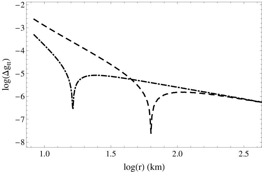
We attempted the same comparison as in [12], assuming the same analytic spacetime and using all numerical models with EOS’s AU, FPS and L, while the quadrupole moment that was inserted in the analytic solution was the one corrected according to Eq. (11). In order to correct it, we used the asymptotic expansion of the metric function of the numerical metric. Although the quadrupole moment was not affected by more than , and for some numerical models by a much lower fraction, the improvement it evoked in matching the numerical metric was almost an order of magnitude. We computed the overall mismatch between the numerical and the analytic metric exterior to the star, which was defined as , where indicate the numerical and the analytic metric components respectively and is the surface radius. The improvement we gained in the overall mismatch was a factor of to for the and to (in most cases) for the . In a few cases the improvement in the mismatch of (and in one model of ) was either marginal or worse after the correction of . This happened because, while we correct the of the Manko et al. metric, its octupole is altered in such a way that the analytic metric finally raises its overall mismatch. However, even these not improved cases have an extremely good overall mismatch (less than 0.004 after the worsening). For a full presentation of the numerical results of the mismatch and the fractional deviation of and due to correction, see [25]. Figure 1 shows an example of the mismatch between analytic and numerical metric functions before and after the correction.


Whenever an analytic metric is used to mimic the gravitational field of a realistic neutron star [13], and then this metric is used to reproduce various observables related to neutron stars [24], it is important to use the right moments in order to build a faithful analytic metric; otherwise any physical conclusion inferred by the analytic metric would be off [23]. If quantitative conclusions are drawn while using wrong moments in the analytic metric, they should be taken into account with some reservation.
(ii) Another important effect of altering the values of the multipole moments of numerical neutron-star models is in relating the higher moments of the compact object with its spin . This was attempted by Laarakkers and Poisson [9] for the quadrupole moment, but due to the omission of the -related term the parameters estimated when relating to were somewhat off. We repeated their analysis with the corrected values of and we got a bit different fitting parameters. In [25] one could find our parameters; however they cannot not be directly compared to the ones of [9] since the sequences of model we used are not exactly equivalent to the ones of [9]. Having the right relations between various moments could help us interpret future accurate observations with connection to the internal structure of neutron stars. At this point we should note that the correcting factor deviates from following a quadratic relation with as well, thus preserving the quadratic fit of with that was found in [9]. Furthermore we found a similar empirical relation for with , namely , with a constant parameter depending on the EOS and the mass of the neutron star (see [25]).
(iii) The ISCO radius, which is significant for a number of astrophysical observations, is intimately related to the exact relativistic moments of the central object, since it lies close to it. In [21] the ISCO of various numerical models of neutron stars were compared to the ISCO computed for a Hartle-Thorne (HT) analytic metric [22], that was suitably constructed to match the behavior of the numerical models. What they found was that although the relative difference in quadrupole between HT and numerical models was oddly high even at slow rotations (where one would expect almost perfect match), the corresponding ISCOs were extremely close (at low spins). This intriguing disagreement disappears for the right quadrupoles of the numerical models. On the other hand the ISCOs were originally in good agreement since they are not affected by such misidentification of and were accurately computed for both metrics. However, that would not be the case if the approximate formula of SS [8] was used to compute the ISCO, since it is a function of the various moments. We repeated the comparison of ISCOs [12] between the numerical one and that obtained from SS and we found a partial improvement but not an impressive one. The reason is that at low quadrupoles (corresponding to low spins) SS’s formula is extremely accurate and quite insensitive to small corrections of , while at high quadrupoles the correction of ISCO through is significant but then the formula deviates a lot from the true ISCO. For example the relative difference of ISCO drops from to (due to correction of ) for low , while it drops from to for a large value of (for a sequence of models of FPS).
(vi) Finally, in [20] the apparent surface area of a rotating neutron star, due to its quadrupole deformation, is computed as a function of this deformation. The deformation parameter though is read from the quadratic fit of [9] which is somewhat distorted due to wrong identification of moments. Hence, the numbers are once again slightly deviated from their true values.
Acknowledgements
We would like to thank N. Stergioulas and K. Kokkotas for helpful and enlightening discussions on the subject. GP would like to thank H. Markakis for the discussions that led us search more deeply the apparent disagreement between numerical models and analytic metrics. The work was supported by the research funding program of I.K.Y. (IKYDA 2010).
References
- [1] R. Geroch, J. Math. Phys. 11, 1955 (1970); 11, 2580 (1970).
- [2] R. O. Hansen, J. Math. Phys. 15, 46 (1974).
- [3] G. Fodor, C. Hoenselaers, and Z. Perjés, J. Math. Phys. 30, 2252 (1989).
- [4] W. Simon and R. Beig, J. Math. Phys. 24, 1163 (1983).
- [5] K. S. Thorne, Rev. Mod. Phys. 52, 299 (1980).
- [6] H. Quevedo, Fortschr. Phys. 38, 733 (1990).
- [7] F. D. Ryan, Phys. Rev. D 52, 5707 (1995).
- [8] M. Shibata and M. Sasaki, Phys. Rev. D 58, 104011 (1998).
- [9] W. G. Laarakkers and E. Poisson, ApJ 512, 282 (1999).
- [10] N. Stergioulas and J. L. Friedman, ApJ 444, 306 (1995); N. Stergioulas, computer code rns, http://www.gravity.phys.uwm.edu/rns.
- [11] V. S. Manko, E. W. Mielke, and J. D. Sanabria-Gómez, Phys. Rev. D 61, 081501 (2000); V. S. Manko, J. D. Sanabria-Gómez, and O. V. Manko, ibid. 62, 044048 (2000).
- [12] E. Berti and N. Stergioulas, MNRAS 350, 1416 (2004).
- [13] G. Pappas, Journal of Physics: Conference Series 189, 012028 (2009); G. Pappas and T. A. Apostolatos, (work in preparation).
- [14] E. M. Butterworth and J. R. Ipser, ApJ 204, 200 (1976).
- [15] H. Komatsu, Y. Eriguchi, and I. Hechisu, MNRAS 237, 355 (1989).
- [16] G. B. Cook, S. L. Shapiro, and S. A. Teukolsky, ApJ 424, 823 (1994).
- [17] F. D. Ryan, Phys. Rev. D 55, 6081 (1997).
- [18] J. L. Friedman and N. Stergioulas, Rotating Relativistic Stars (Cambridge Monographs on Mathematical Physics, in press).
- [19] A. Lanza, Class. Quantum Grav. 9, 677 (1992).
- [20] M. Baubock, D. Psaltis, F. Ozel, and T. Johannsen, arXiv:1110.4389.
- [21] E. Berti, F. White, A. Maniopoulou, M. Bruni, MNRAS 358, 923 (2005).
- [22] J. B. Hartle and K. S. Thorne, ApJ 153, 807 (1968).
- [23] L. A. Pachn, J.A. Rueda, J. D. Sanabria-Gomez, Phys. Rev. D 73, 104038 (2006).
- [24] G. Pappas, (work in preparation)
- [25] See Supplemental Material.
V Supplemental material
V.1 Preliminary remarks
In this supplement, we give a detailed account of all data related to the neutron star models that we used in our analysis and all the results from the comparisons between using the previously assumed moments and the corrected ones.
For our analysis we have constructed several numerical neutron star models, using Stergioulas’ “rns” code [10]. Specifically, we have constructed the same models as the ones presented in [12] for the equations of state AU, FPS and L. These models correspond to sequences of constant baryonic mass with varying rotation. In particular we have: (i) one sequence which corresponds to a non-rotating model of mass , (ii) one sequence which corresponds to the non-rotating model of maximum mass for the particular equation of state, and (iii) a sequence that doesn’t have a non-rotating limit. Every sequence consists of 10 models, so we have studied 30 models for every equation of state.
V.2 Fitting parameters for higher multipoles vs spin
We have tried to fit the reduced quadrupole mass-moment and the reduced octupole current-mass moment with simple polynomials of the spin parameter , for every sequence of the numerical neutron-star models that were briefly presented in the previous section. The moments and are obtained from the “rns” code and corrected according to Eq. (11) of our letter. The dimensionless parameter was fitted as a pure quadratic polynomial of the spin parameter for all three sequences, and additionally in the case of sequence (iii) as a polynomial of the form to improve the fit. Accordingly the octupole parameter was fitted by a pure cubic fit for all sequences, and in the case of sequence (iii) as a polynomial of the form . In Fig. 2 we present the data for and as functions of the spin parameter, as well as the corresponding best-fit polynomials. In Table 1 the corresponding fitting parameters are shown for each sequence of models and for each EOS. Furthermore we investigated the behavior of with , since the value affects the correction in and in a linear fashion. We found that follows a quadratic relation with as well; the correction preserves the quadratic relation of found in [9]. The plots and the corresponding best fits for are also shown in Fig. 2, and the fitting parameters are written in Table 1.
| AU | FPS | L | |||||||
| - | - | -0.25 | - | - | -0.25 | - | - | -0.25 | |
| - | - | - | - | - | - | - | - | - | |
| -3.83 | - | 0.11 | -4.22 | - | 0.11 | -7.42 | - | 0.08 | |
| - | -7.38 | - | - | -8.45 | - | - | -15.38 | - | |
| - | - | -0.25 | - | - | -0.25 | - | - | -0.25 | |
| - | - | - | - | - | - | - | - | - | |
| -1.61 | - | 0.17 | -2.33 | - | 0.14 | -2.19 | - | 0.14 | |
| - | -2.41 | - | - | -4.14 | - | - | -3.75 | - | |
| - | - | -0.24 | - | - | -0.24 | - | - | -0.24 | |
| - | - | - | - | - | - | - | - | - | |
| -1.41 | - | 0.16 | -1.97 | - | 0.13 | -1.83 | - | 0.14 | |
| - | -1.98 | - | - | -3.39 | - | - | -2.98 | - | |
| - | - | -0.24 | - | - | -0.24 | - | - | -0.24 | |
| 0.40 | - | - | 0.61 | - | - | 0.54 | - | - | |
| -2.07 | 0.96 | 0.16 | -3.06 | 1.5 | 0.13 | -2.74 | 1.29 | 0.14 | |
| - | -3.50 | - | - | -5.93 | - | - | -5.06 | - |


V.3 Matching a neutron-star spacetime with a Manko et al. metric
We have compared the metric functions and on the equatorial plane of various numerical models of neutron stars (the same sequences and EOSs presented in Sec. V.1) with the corresponding Manko et al. [11] metric functions. For every star the analytic metric was constructed with the same mass , and spin , as the numerical model, while the third parameter of the analytic solution was adjusted so as its quadrupole moment equals the quadrupole moment of the numerical spacetime. That was attempted both when the correction in was omitted (as in [12]), and when the correction was taken into account. For every numerical model we recorded the first four non-vanishing multipole moments, as well as the fractional difference in and due to correction. We also give the parameter as evaluated from the numerical metric. The numbers are shown in Tables 2, 4, 6 (the spin parameter is shown instead of the angular momentum ).
In Tables 3, 5, 7 we present the results of the comparison between the numerical metric functions and the corresponding analytic ones. More specifically we give: (a) the overall mismatch and with the corrected value for , (b) the improvements in the overall mismatch due to correction,
and (c) the fractional difference in of the Manko et al. metric (which, for this particular analytic spacetime, depends on the first three multipole moments) due to the correction in . We should note that in the case of the Manko et al. metric, the quadrupole can not take arbitrarily low values; thus not every numerical model has a corresponding analytic model. We indicate the specific models in Tables 3, 5, 7 by their numbering in Tables 2, 4, 6, respectively.
Finally in Figures 3, 4, 5, we have plotted for one model of each sequence and each EOS the fractional difference between the actual numerical metric functions and the corresponding Manko et al. metric functions both when the analytic metrics were built with the wrong and with the right quadrupole moment. These plots show graphically the improvement caused by the correction of the quadrupole moment. We should note that in the cases that the correction in the quadrupole is small (which corresponds to the first sequences of all EOSs), the mismatch between the analytic and the numerical metric component is slightly worse after the correction. That effect is discussed in the main text. As it can be seen though, the mismatch both before and after the correction is relatively small in these cases.
| (%) | (%) | ||||||
|---|---|---|---|---|---|---|---|
| 1 | 2.069 | 0. | 0. | 0. | -0.25 | - | - |
| 2 | 2.072 | 0.201 | -1.45 | -1.14 | -0.24 | 3.956 | 3.756 |
| 3 | 2.078 | 0.312 | -3.47 | -4.28 | -0.23 | 3.993 | 3.779 |
| 4 | 2.087 | 0.414 | -6.08 | -10.0 | -0.23 | 4.032 | 3.805 |
| 5 | 2.092 | 0.474 | -7.99 | -15.1 | -0.22 | 4.038 | 3.799 |
| 6 | 2.097 | 0.529 | -9.96 | -21.2 | -0.21 | 4.044 | 3.792 |
| 7 | 2.103 | 0.578 | -11.9 | -27.9 | -0.21 | 4.041 | 3.775 |
| 8 | 2.108 | 0.616 | -13.6 | -34.1 | -0.20 | 4.029 | 3.751 |
| 9 | 2.111 | 0.650 | -15.2 | -40.5 | -0.20 | 4.008 | 3.716 |
| 10 | 2.112 | 0.661 | -15.7 | -42.7 | -0.20 | 4.002 | 3.706 |
| 11 | 3.151 | 0. | 0. | 0. | -0.25 | - | - |
| 12 | 3.164 | 0.194 | -1.68 | -1.37 | -0.24 | 21.63 | 31.69 |
| 13 | 3.183 | 0.309 | -4.46 | -5.97 | -0.23 | 20.41 | 28.99 |
| 14 | 3.207 | 0.406 | -8.08 | -14.5 | -0.22 | 19.35 | 26.72 |
| 15 | 3.231 | 0.485 | -12.0 | -26.6 | -0.20 | 18.43 | 24.82 |
| 16 | 3.253 | 0.550 | -16.1 | -41.4 | -0.19 | 17.62 | 23.18 |
| 17 | 3.273 | 0.603 | -20.2 | -58.1 | -0.18 | 16.92 | 21.80 |
| 18 | 3.291 | 0.645 | -23.9 | -75.1 | -0.17 | 16.33 | 20.67 |
| 19 | 3.304 | 0.676 | -27.0 | -90.4 | -0.17 | 15.86 | 19.77 |
| 20 | 3.318 | 0.706 | -30.3 | -107. | -0.16 | 15.40 | 18.88 |
| 21 | 3.388 | 0.510 | -12.8 | -27.8 | -0.19 | 26.05 | 42.10 |
| 22 | 3.388 | 0.510 | -12.9 | -28.1 | -0.19 | 25.75 | 41.32 |
| 23 | 3.390 | 0.514 | -13.2 | -29.3 | -0.19 | 25.17 | 39.83 |
| 24 | 3.393 | 0.520 | -13.7 | -31.1 | -0.19 | 24.60 | 38.38 |
| 25 | 3.405 | 0.547 | -15.8 | -38.7 | -0.19 | 23.18 | 34.89 |
| 26 | 3.422 | 0.587 | -19.1 | -51.6 | -0.18 | 21.76 | 31.57 |
| 27 | 3.441 | 0.626 | -22.7 | -67.1 | -0.17 | 20.65 | 29.07 |
| 28 | 3.458 | 0.659 | -26.0 | -82.7 | -0.17 | 19.79 | 27.20 |
| 29 | 3.477 | 0.694 | -30.1 | -103. | -0.16 | 18.91 | 25.31 |
| 30 | 3.487 | 0.713 | -32.5 | -115. | -0.16 | 18.45 | 24.34 |
| (%) | |||||
| 3 | 7.319 | 4.760 | 0.00004 | 0.42877 | 0.00115 |
| 4 | 5.474 | 5.150 | 0.00007 | 0.70046 | 0.00376 |
| 5 | 5.159 | 3.690 | 0.00014 | 0.67202 | 0.00447 |
| 6 | 4.981 | 2.928 | 0.00022 | 0.59514 | 0.00437 |
| 7 | 4.857 | 2.506 | 0.00032 | 0.44967 | 0.00360 |
| 8 | 4.770 | 2.294 | 0.00039 | 0.26800 | 0.00260 |
| 9 | 4.690 | 2.169 | 0.00044 | 0.73064 | 0.00149 |
| 10 | 4.668 | 2.150 | 0.00044 | 1.20269 | 0.00117 |
| 18 | 24.26 | 7.692 | 0.00068 | 6.4051 | 0.00627 |
| 19 | 22.60 | 6.834 | 0.00078 | 5.61239 | 0.00728 |
| 20 | 21.32 | 6.577 | 0.00073 | 4.94567 | 0.00766 |
| 29 | 27.99 | 7.985 | 0.00088 | 5.34521 | 0.01141 |
| 30 | 26.49 | 8.058 | 0.00078 | 5.16811 | 0.01051 |
| (%) | (%) | ||||||
|---|---|---|---|---|---|---|---|
| 1 | 2.067 | 0. | 0 | 0 | -0.25 | - | - |
| 2 | 2.071 | 0.201 | -1.54 | -1.25 | -0.24 | 3.691 | 3.404 |
| 3 | 2.077 | 0.301 | -3.45 | -4.22 | -0.23 | 3.685 | 3.385 |
| 4 | 2.083 | 0.385 | -5.64 | -8.88 | -0.23 | 3.667 | 3.355 |
| 5 | 2.087 | 0.452 | -7.85 | -14.6 | -0.22 | 3.634 | 3.311 |
| 6 | 2.093 | 0.507 | -9.94 | -20.9 | -0.22 | 3.610 | 3.275 |
| 7 | 2.098 | 0.557 | -12.0 | -28.0 | -0.21 | 3.575 | 3.228 |
| 8 | 2.102 | 0.603 | -14.2 | -36.1 | -0.21 | 3.532 | 3.173 |
| 9 | 2.106 | 0.636 | -15.9 | -42.9 | -0.20 | 3.504 | 3.136 |
| 10 | 2.109 | 0.666 | -17.6 | -49.9 | -0.20 | 3.469 | 3.091 |
| 11 | 2.658 | 0. | 0 | 0 | -0.25 | - | - |
| 12 | 2.664 | 0.163 | -0.94 | -0.64 | -0.24 | 13.74 | 16.07 |
| 13 | 2.674 | 0.260 | -2.51 | -2.81 | -0.23 | 12.65 | 14.41 |
| 14 | 2.686 | 0.349 | -4.81 | -7.43 | -0.23 | 11.63 | 12.90 |
| 15 | 2.701 | 0.436 | -8.00 | -15.8 | -0.22 | 10.69 | 11.56 |
| 16 | 2.714 | 0.500 | -11.0 | -25.6 | -0.21 | 10.05 | 10.65 |
| 17 | 2.727 | 0.562 | -14.6 | -39.0 | -0.20 | 9.428 | 9.805 |
| 18 | 2.736 | 0.602 | -17.4 | -50.4 | -0.19 | 9.026 | 9.261 |
| 19 | 2.744 | 0.633 | -19.7 | -60.8 | -0.19 | 8.734 | 8.866 |
| 20 | 2.750 | 0.654 | -21.4 | -69.0 | -0.18 | 8.543 | 8.607 |
| 21 | 2.823 | 0.427 | -6.54 | -11.7 | -0.21 | 17.55 | 22.14 |
| 22 | 2.823 | 0.428 | -6.69 | -12.1 | -0.21 | 16.97 | 21.12 |
| 23 | 2.825 | 0.432 | -6.98 | -12.9 | -0.21 | 16.40 | 20.16 |
| 24 | 2.826 | 0.439 | -7.35 | -13.9 | -0.21 | 15.84 | 19.22 |
| 25 | 2.829 | 0.450 | -7.88 | -15.4 | -0.21 | 15.30 | 18.34 |
| 26 | 2.840 | 0.492 | -10.1 | -22.5 | -0.20 | 13.76 | 15.88 |
| 27 | 2.856 | 0.552 | -13.8 | -35.7 | -0.20 | 12.35 | 13.73 |
| 28 | 2.871 | 0.609 | -17.9 | -52.9 | -0.19 | 11.25 | 12.13 |
| 29 | 2.882 | 0.647 | -21.1 | -67.6 | -0.18 | 10.64 | 11.25 |
| 30 | 2.884 | 0.658 | -22.2 | -72.8 | -0.18 | 10.42 | 10.94 |
| (%) | |||||
| 3 | 6.730 | 4.062 | 0.00003 | 0.46717 | 0.00096 |
| 4 | 5.056 | 4.805 | 0.00005 | 0.72818 | 0.00297 |
| 5 | 4.633 | 3.397 | 0.00012 | 0.71192 | 0.00380 |
| 6 | 4.423 | 2.699 | 0.00020 | 0.64891 | 0.00377 |
| 7 | 4.266 | 2.314 | 0.00028 | 0.52289 | 0.00311 |
| 8 | 4.134 | 2.090 | 0.00036 | 0.30332 | 0.00201 |
| 9 | 4.057 | 2.003 | 0.00039 | 0.84777 | 0.00108 |
| 10 | 3.980 | 2.040 | 0.00033 | 2.86108 | 0.00052 |
| 16 | 15.28 | 6.508 | 0.00024 | 15.13 | 0.00047 |
| 17 | 13.00 | 4.908 | 0.00037 | 9.12807 | 0.00085 |
| 18 | 11.97 | 4.140 | 0.00047 | 7.78352 | 0.00116 |
| 19 | 11.31 | 3.745 | 0.00053 | 4.9739 | 0.00203 |
| 20 | 10.90 | 3.613 | 0.00053 | 3.90644 | 0.00266 |
| 27 | 18.56 | 6.396 | 0.00038 | 6.08298 | 0.00238 |
| 28 | 15.49 | 4.938 | 0.00052 | 5.20018 | 0.00288 |
| 29 | 14.13 | 4.374 | 0.00057 | 3.92533 | 0.00392 |
| 30 | 13.69 | 4.374 | 0.00053 | 3.71457 | 0.00392 |
| (%) | (%) | ||||||
|---|---|---|---|---|---|---|---|
| 1 | 2.080 | 0. | 0 | 0 | -0.25 | - | - |
| 2 | 2.071 | 0.194 | -2.76 | -2.28 | -0.24 | 1.302 | 1.136 |
| 3 | 2.075 | 0.324 | -7.55 | -10.5 | -0.24 | 1.328 | 1.156 |
| 4 | 2.080 | 0.417 | -12.2 | -22.0 | -0.23 | 1.352 | 1.175 |
| 5 | 2.083 | 0.483 | -16.2 | -33.9 | -0.23 | 1.369 | 1.188 |
| 6 | 2.087 | 0.543 | -20.3 | -47.9 | -0.22 | 1.387 | 1.201 |
| 7 | 2.090 | 0.598 | -24.4 | -63.5 | -0.22 | 1.399 | 1.210 |
| 8 | 2.095 | 0.650 | -28.6 | -81.3 | -0.21 | 1.412 | 1.218 |
| 9 | 2.096 | 0.690 | -32.1 | -97.1 | -0.21 | 1.417 | 1.220 |
| 10 | 2.097 | 0.698 | -32.9 | -100. | -0.21 | 1.420 | 1.222 |
| 11 | 3.995 | 0. | 0 | 0 | -0.25 | - | - |
| 12 | 4.012 | 0.178 | -3.80 | -4.23 | -0.24 | 13.65 | 16.18 |
| 13 | 4.029 | 0.280 | -9.84 | -17.5 | -0.23 | 12.72 | 14.74 |
| 14 | 4.051 | 0.375 | -18.5 | -45.4 | -0.22 | 11.94 | 13.57 |
| 15 | 4.074 | 0.458 | -29.0 | -88.4 | -0.21 | 11.28 | 12.59 |
| 16 | 4.098 | 0.528 | -40.3 | -144. | -0.20 | 10.72 | 11.77 |
| 17 | 4.120 | 0.588 | -51.8 | -210. | -0.19 | 10.25 | 11.09 |
| 18 | 4.139 | 0.635 | -62.6 | -279. | -0.19 | 9.865 | 10.54 |
| 19 | 4.160 | 0.682 | -74.9 | -365. | -0.18 | 9.478 | 9.998 |
| 20 | 4.167 | 0.700 | -79.8 | -401. | -0.17 | 9.335 | 9.794 |
| 21 | 4.321 | 0.478 | -29.0 | -88.0 | -0.20 | 17.68 | 22.66 |
| 22 | 4.321 | 0.479 | -29.5 | -90.2 | -0.20 | 17.19 | 21.82 |
| 23 | 4.324 | 0.483 | -30.7 | -95.7 | -0.20 | 16.66 | 20.90 |
| 24 | 4.325 | 0.489 | -31.9 | -101. | -0.20 | 16.24 | 20.20 |
| 25 | 4.333 | 0.505 | -35.0 | -116. | -0.20 | 15.55 | 19.03 |
| 26 | 4.355 | 0.555 | -45.2 | -170. | -0.19 | 14.17 | 16.79 |
| 27 | 4.377 | 0.602 | -55.9 | -233. | -0.19 | 13.27 | 15.36 |
| 28 | 4.396 | 0.641 | -66.0 | -299. | -0.18 | 12.60 | 14.32 |
| 29 | 4.418 | 0.684 | -78.7 | -389. | -0.17 | 11.92 | 13.28 |
| 30 | 4.420 | 0.686 | -79.4 | -394. | -0.17 | 11.89 | 13.24 |
| (%) | |||||
| 2 | 3.364 | 0.846 | 0.00002 | 0.81731 | 0.00034 |
| 3 | 1.677 | 2.888 | 0.00002 | 0.94960 | 0.00328 |
| 4 | 1.579 | 2.017 | 0.00007 | 0.94067 | 0.00473 |
| 5 | 1.550 | 1.679 | 0.00014 | 0.92563 | 0.00500 |
| 6 | 1.540 | 1.519 | 0.00022 | 0.90005 | 0.00459 |
| 7 | 1.534 | 1.431 | 0.00030 | 0.85334 | 0.00360 |
| 8 | 1.535 | 1.377 | 0.00038 | 0.74334 | 0.00221 |
| 9 | 1.533 | 1.355 | 0.00041 | 0.61091 | 0.00102 |
| 10 | 1.534 | 1.354 | 0.00041 | 0.72087 | 0.00082 |
| 16 | 16.01 | 6.594 | 0.00039 | 11.1166 | 0.00158 |
| 17 | 14.15 | 5.081 | 0.00060 | 9.2408 | 0.00221 |
| 18 | 13.08 | 4.119 | 0.00083 | 7.25373 | 0.00347 |
| 19 | 12.18 | 3.520 | 0.00102 | 3.86123 | 0.00792 |
| 20 | 11.87 | 3.397 | 0.00104 | 3.31502 | 0.00960 |
| 26 | 23.13 | 7.416 | 0.00054 | 5.91821 | 0.00682 |
| 27 | 19.25 | 6.100 | 0.00071 | 6.64409 | 0.00600 |
| 28 | 17.44 | 5.094 | 0.00090 | 5.33573 | 0.00802 |
| 29 | 15.89 | 4.316 | 0.00108 | 3.84442 | 0.01207 |
| 30 | 15.82 | 4.286 | 0.00108 | 3.79143 | 0.01227 |




V.4 Results for the
For the assessment of the implications the correction in the multipole moments has, we have also calculated its effect on the location of the radius of the innermost stable circular orbit . The ISCO of the co-rotating orbits for the numerical neutron star models is directly computed by the “rns” code. For every model we have computed the ISCOs for the analytic metric of Manko et al. using the wrong quadrupole and the corrected one. The same is repeated using the formula of Shibata and Sasaki [8] up to terms corresponding to the octupole current-mass moment (as it was done in [12]).
Tables 8, 9, 10, show our results for the , namely the numerical ISCO, the Manko et al. ISCO, before and after the correction in the quadrupole, and the Shibata and Sasaki ISCO, again before and after the correction. The models for which there is no value for the numerical , correspond to neutron stars that have their ISCO below the star’s surface. The models that do not have analytic correspond to cases for which no analytic metric can be found to match their numerical quadrupole.
The calculated from the Manko et al. metric is relatively close to the numerical one before the correction and it gets even closer after the correction. As discussed in the text, the ISCO calculated from the Shibata and Sasaki formula is already a good approximation, before the correction, of the numerical one for slow rotation, and improves slightly after the correction. On the other hand, for higher rotation the improvement is greater but then the approximate formula is insufficient to describe so rapidly rotating stars, at least up to the approximation used.
| 1 | 12.41 | - | - | 12.41 | 12.41 |
|---|---|---|---|---|---|
| 2 | 11.36 | - | - | 11.30 | 11.32 |
| 3 | 11.11 | 11.02 | 11.05 | 10.89 | 10.93 |
| 4 | - | 10.84 | 10.89 | 10.63 | 10.69 |
| 5 | - | 10.80 | 10.87 | 10.50 | 10.59 |
| 6 | - | 10.82 | 10.91 | 10.41 | 10.52 |
| 7 | - | 10.88 | 10.98 | 10.35 | 10.48 |
| 8 | - | 10.94 | 11.06 | 10.31 | 10.47 |
| 9 | - | 11.02 | 11.14 | 10.28 | 10.45 |
| 10 | - | 11.05 | 11.17 | 10.27 | 10.45 |
| 11 | 18.91 | - | - | 18.91 | 18.91 |
| 12 | 17.00 | - | - | 16.94 | 16.97 |
| 13 | 15.97 | - | - | 15.76 | 15.83 |
| 14 | 15.21 | - | - | 14.73 | 14.86 |
| 15 | 14.68 | - | - | 13.86 | 14.03 |
| 16 | 14.35 | - | - | 13.10 | 13.31 |
| 17 | 14.16 | - | - | 12.44 | 12.68 |
| 18 | 14.08 | 13.42 | 13.91 | 11.88 | 12.15 |
| 19 | 14.08 | 13.29 | 13.83 | 11.44 | 11.74 |
| 20 | 14.12 | 13.20 | 13.79 | 11.01 | 11.32 |
| 21 | 14.80 | - | - | 13.99 | 14.19 |
| 22 | 14.81 | - | - | 13.99 | 14.19 |
| 23 | 14.80 | - | - | 13.95 | 14.16 |
| 24 | 14.77 | - | - | 13.88 | 14.09 |
| 25 | 14.64 | - | - | 13.55 | 13.77 |
| 26 | 14.45 | - | - | 13.03 | 13.28 |
| 27 | 14.31 | - | - | 12.49 | 12.76 |
| 28 | 14.24 | - | - | 12.02 | 12.31 |
| 29 | 14.23 | 13.36 | 14.04 | 11.48 | 11.79 |
| 30 | 14.25 | 13.28 | 14.01 | 11.18 | 11.50 |
| 1 | 12.40 | - | - | 12.40 | 12.40 |
|---|---|---|---|---|---|
| 2 | 11.38 | - | - | 11.31 | 11.33 |
| 3 | - | 11.09 | 11.12 | 10.98 | 11.01 |
| 4 | - | 10.96 | 11.00 | 10.78 | 10.83 |
| 5 | - | 10.93 | 10.99 | 10.67 | 10.75 |
| 6 | - | 10.98 | 11.06 | 10.62 | 10.72 |
| 7 | - | 11.06 | 11.15 | 10.60 | 10.72 |
| 8 | - | 11.18 | 11.28 | 10.60 | 10.74 |
| 9 | - | 11.28 | 11.39 | 10.61 | 10.77 |
| 10 | - | 11.40 | 11.51 | 10.63 | 10.80 |
| 11 | 15.94 | - | - | 15.94 | 15.94 |
| 12 | 14.61 | - | - | 14.58 | 14.59 |
| 13 | 13.94 | - | - | 13.81 | 13.86 |
| 14 | 13.44 | - | - | 13.13 | 13.20 |
| 15 | 13.11 | - | - | 12.47 | 12.59 |
| 16 | 13.00 | 12.70 | 12.87 | 11.99 | 12.14 |
| 17 | 13.04 | 12.55 | 12.77 | 11.52 | 11.71 |
| 18 | 13.14 | 12.52 | 12.76 | 11.21 | 11.42 |
| 19 | 13.27 | 12.53 | 12.78 | 10.97 | 11.19 |
| 20 | - | 12.55 | 12.82 | 10.80 | 11.04 |
| 21 | 13.32 | - | - | 12.83 | 12.96 |
| 22 | 13.33 | - | - | 12.84 | 12.97 |
| 23 | 13.34 | - | - | 12.81 | 12.94 |
| 24 | 13.33 | - | - | 12.77 | 12.90 |
| 25 | 13.30 | - | - | 12.69 | 12.83 |
| 26 | 13.21 | - | - | 12.34 | 12.50 |
| 27 | 13.17 | 12.78 | 13.02 | 11.84 | 12.03 |
| 28 | 13.27 | 12.68 | 12.98 | 11.33 | 11.56 |
| 29 | 13.43 | 12.68 | 13.00 | 10.99 | 11.24 |
| 30 | - | 12.69 | 13.02 | 10.87 | 11.13 |
| 1 | - | - | - | 12.48 | 12.48 |
|---|---|---|---|---|---|
| 2 | - | 11.73 | 11.74 | 11.69 | 11.70 |
| 3 | - | 11.80 | 11.82 | 11.84 | 11.87 |
| 4 | - | 12.09 | 12.12 | 12.20 | 12.25 |
| 5 | - | 12.38 | 12.41 | 12.57 | 12.63 |
| 6 | - | 12.69 | 12.74 | 12.98 | 13.06 |
| 7 | - | 13.01 | 13.06 | 13.40 | 13.50 |
| 8 | - | 13.34 | 13.40 | 13.85 | 13.97 |
| 9 | - | 13.61 | 13.67 | 14.22 | 14.36 |
| 10 | - | 13.67 | 13.73 | 14.30 | 14.44 |
| 11 | 23.97 | - | - | 23.97 | 23.97 |
| 12 | 21.83 | - | - | 21.74 | 21.77 |
| 13 | 20.78 | - | - | 20.45 | 20.51 |
| 14 | 20.00 | - | - | 19.17 | 19.27 |
| 15 | 19.52 | - | - | 17.96 | 18.09 |
| 16 | 19.32 | 18.80 | 19.1 | 16.81 | 16.96 |
| 17 | 19.32 | 18.56 | 18.92 | 15.71 | 15.89 |
| 18 | 19.46 | 18.46 | 18.88 | 14.73 | 14.92 |
| 19 | 19.73 | 18.46 | 18.94 | 13.63 | 13.82 |
| 20 | 19.87 | 18.49 | 18.98 | 13.19 | 13.39 |
| 21 | 19.81 | - | - | 18.37 | 18.52 |
| 22 | 19.84 | - | - | 18.37 | 18.52 |
| 23 | 19.85 | - | - | 18.30 | 18.45 |
| 24 | 19.85 | - | - | 18.21 | 18.37 |
| 25 | 19.80 | - | - | 17.94 | 18.10 |
| 26 | 19.68 | 19.15 | 19.54 | 16.99 | 17.16 |
| 27 | 19.67 | 18.90 | 19.39 | 16.03 | 16.21 |
| 28 | 19.76 | 18.78 | 19.33 | 15.13 | 15.31 |
| 29 | 19.98 | 18.74 | 19.35 | 14.02 | 14.20 |
| 30 | 19.99 | 18.74 | 19.35 | 13.96 | 14.14 |