Mean exit time and escape probability for dynamical systems driven by Lévy noise
Abstract
The mean first exit time and escape probability are utilized to quantify dynamical behaviors of stochastic differential equations with non-Gaussian stable type Lévy motions. Both deterministic quantities are characterized by differential-integral equations (i.e., differential equations with nonlocal terms) but with different exterior conditions. The non-Gaussianity of noises manifests as nonlocality at the level of mean exit time and escape probability. An objective of this paper is to make mean exit time and escape probability as efficient computational tools, to the applied probability community, for quantifying stochastic dynamics. An accurate numerical scheme is developed and validated for computing the mean exit time and escape probability. Asymptotic solution for the mean exit time is given when the pure jump measure in the Lévy motion is small.
From both the analytical and numerical results, it is observed that the mean exit time depends strongly on the domain size and the value of in the stable Lévy jump measure. The mean exit time can measure which of the two competing factors in -stable Lévy motion, i.e. the jump frequency or the jump size, is dominant in helping a process exit a bounded domain. The escape probability is shown to vary with the underlying vector field (i.e., drift). The mean exit time and escape probability could become discontinuous at the boundary of the domain, when the process is subject to certain deterministic potential and the value of is in .
Key Words: Stochastic dynamical systems; non-Gaussian Lévy motion; Lévy jump measure; First exit time; double-well system
Mathematics Subject Classifications (2000): 60H15, 60F10, 60G17
1 Motivation
Random fluctuations in complex systems in engineering and science are often non-Gaussian [28, 9, 10]. For instance, it has been argued that diffusion by geophysical turbulence [26] corresponds, loosely speaking, to a series of “pauses”, when the particle is trapped by a coherent structure, and “flights” or “jumps” or other extreme events, when the particle moves in the jet flow. Paleoclimatic data [11] also indicate such irregular processes.
Lévy motions are thought to be appropriate models for non-Gaussian processes with jumps [23]. Recall that a Lévy motion , or , is a stochastic process with stationary and independent increments. That is, for any with , the distribution of only depends on , and for any , , , are independent. Without loss of generality, we may assume that the sample paths of are almost surely right continuous with left limits.
This generalizes the Brownian motion , which satisfies all these three conditions. But additionally, (i) almost all sample paths of the Brownian motion are continuous in time in the usual sense and (ii) Brownian motion’s increments are Gaussian distributed.
Stochastic differential equations (SDEs) with non-Gaussian Lévy noises have attracted much attention recently [2, 24]. To be specific, let us consider the following scalar SDE with a non-Gaussian Lévy motion
| (1) |
where is a vector field (or drift), and is a scalar Lévy motion defined in a probability space .
We study the first exit problem for the solution process from bounded domains. The exit phenomenon, i.e., escaping from a bounded domain in state space, is an impact of randomness on the evolution of such dynamical systems. Two concepts are applied to quantify the exit phenomenon: mean exit time and escape probability.
We define the first exit time from the spatial domain as follows:
and the mean exit time is denoted as . The likelihood of a particle (or a solution path ), starting at a point , first escapes a domain and lands in a subset of (the complement of ) is called escape probability and is denoted as .
The existing work on mean exit time gives asymptotic estimate for when the noise intensity is sufficiently small, i.e., the noise term in (1) is with . See, for example, Imkeller and Pavlyukevich [15, 16], and Yang and Duan [29].
In the present paper, however, we numerically investigate mean exit time and escape probability for arbitrary noise intensity. The mean exit time and escape probability for a dynamical system, driven by a non-Gaussian, discontinuous (with jumps) Lévy motion, are described by two similar differential-integral equations but with different exterior conditions. The non-Gaussianity of the noise manifests as nonlocality at the level of the mean exit time and escape probability. We consider a numerical approach for solving these differential-integral (non-local) equations. A computational analysis is conducted to investigate the relative importance of jump measure, diffusion coefficient and non-Gaussianity in affecting mean exit time and escape probability.
Our goal is to make mean exit time and escape probability as efficient computational tools, to the applied probability community, for quantifying stochastic dynamics.
This paper is organized as follows. In section 2, we recall the generators for Lévy motions. In section 3, we consider SDEs driven by a combination of Brownian motion and a symmetric stable process. Numerical approaches and simulation results are presented in section 4 and 5, respectively. Finally, the results are summarized in section 6.
2 Lévy motion
A scalar Lévy motion is characterized by a linear coefficient , a diffusion parameter and a non-negative Borel measure , defined on and concentrated on , which satisfies
| (2) |
or equivalently
| (3) |
This measure is the so called the Lévy jump measure of the Lévy motion . We also call the generating triplet.
Let be a Lévy process with the generating triplet . It is known that a scalar Lévy motion is completely determined by the Lévy-Khintchine formula (See [2, 23, 22]). This says that for any one-dimensional Lévy process , there exists a , and a measure such that
| (4) |
where is the indicator function of the set , i.e., it takes value on this set and takes zero value otherwise:
The generator of the process is defined as where and is any function belonging to the domain of the operator . Recall that the space of functions with bounded derivatives up to order 2 is contained in the domain of , and that for every (See [2, 22])
| (5) |
Moreover, the generator for the process in (1) is then
| (6) | |||||
3 Mean exit time and escape probability
Now we consider the SDE (1) with a Lévy motion that has the generating triplet , i.e., zero linear coefficient, diffusion coefficient and Lévy measure , with . This Lévy motion is the independent sum of a Brownian motion and a symmetric -stable process. Here is a non-negative parameter and it does not have to be sufficiently small. Strictly speaking, this is not a stable Lévy motion (because the diffusion may be nonzero), but a Lévy motion whose jump measure is the same as that of a stable Lévy motion.
We first consider the mean exit time, , for an orbit starting at , from a bounded interval . By the Dynkin formula [2, 23] for Markov processes, as in [19, 25, 21], we obtain that satisfies the following differential-integral equation:
| (7) | |||
where the generator is
| (8) | |||||
and is the complement set of .
We also consider the escape probability of a particle whose motion is described by the SDE (1). The likelihood of a particle, starting at a point , first escapes a domain and lands in a subset of (the complement of ) is called escape probability. This escape probability, denoted by , satisfies [18, 27] the following equation
| (9) | |||||
where is the generator defined in (8).
In the present paper, we only consider scalar SDEs. For SDEs in higher dimensions, both mean exit time and escape probability will satisfy partial differential-integral equations, and our approaches generally apply.
4 Numerical schemes
Noting the principal value of the integral always vanishes for any , we will choose the value of in Eq. (7) differently according to the value of . Eq. (7) becomes
| (10) |
for ; and for .
Numerical approaches for the mean exit time and escape probability in the SDEs with Brownian motions were considered in [6, 7], among others. In the following, we describe the numerical algorithms for the special case of for clarity of the presentation. The corresponding schemes for the general case can be extended easily. Because vanishes outside , Eq. (10) can be simplified by writing ,
| (11) |
for ; and for .
Noting is not smooth at the boundary points , in order to ensure the integrand is smooth, we rewrite Eq. (11) as
| (12) | |||||
for , and
| (13) | |||||
for . We have chosen .
Let’s divide the interval into sub-intervals and define for integer, where . We denote the numerical solution of at by . Let’s discretize the integral-differential equation (12) using central difference for derivatives and “punched-hole” trapezoidal rule
| (14) |
where . The modified summation symbol means that the quantities corresponding to the two end summation indices are multiplied by .
| (15) |
where . The boundary conditions require that the values of vanish if the index .
The truncation errors of the central differencing schemes for derivatives in (14) and (15) are of 2nd-order . From the error analysis of Navot (1961) [20], the leading-order error of the quadrature rule is , where is the Riemann zeta function. Thus, the following scheme have 2nd-order accuracy for any ,
| (16) |
where . Similarly, for ,
| (17) |
where . if .
We solve the linear system (16-17) by direct LU factorization or the Krylov subspace iterative method GMRES.
We find that the desingularizing term () does not have any effect on the numerical results, regardless whether we use LU or GMRES for solving the linear system. In this case, we can discretize the following equation instead of (11)
| (18) |
where the integral in the equation is taken as Cauchy principal value integral. Consequently, instead of (16) and (17), we have only one discretized equation for any and
| (19) |
With minor changes, we also have the scheme for simulating escape probability characterized by the equation (9).
5 Numerical results
5.1 Verification
5.1.1 Comparing with analytical solutions
In order to verify that the numerical integration scheme for treating the improper integral in (7) is implemented correctly, we compute the left-hand side(LHS) of (7) by substituting , , and
| (20) |

Figure 1 shows the differences (the errors) between the numerical and the analytical values of LHS of (7) at the fixed value for different resolutions and . We plot against for , where and is the difference between the numerical and the analytical values of LHS. Clearly, the numerical results show that the error of computing LHS decays as . The second-order accuracy is expected from the error analysis of the numerical integration method (19). For a fixed resolution , the error increases as increases due to the fact that LHS in (20) becomes more singular at and as increases.

Next, we compare the numerical solution with the analytical solution for the mean exit time [13]
| (21) |
in the special case of (7) in which , , and with . Figure 2 shows the numerical solutions (the dashed lines) obtained by solving the discretized equations (16) and (17) or (19) with the fixed resolution , and different values of , while the corresponding analytical solutions are shown with the solid lines. The comparison shows that the numerical solutions are very accurate as one can hardly distinguish the numerical solution from the corresponding analytical one. Note that, in this case of , for a fixed value of the starting point , the mean exit time decreases when increases in the interval . Later, we will see the dependence of the mean exit time on is much more complicated when the size of the interval is increased.

Figure 3 gives the error in the numerical solution to the discretized equations (14) and (15) derived by using ”punched-hole” trapezoidal rule. Here, we compute by comparing the mean exit time at for different resolutions and values of , where and denotes the analytical and the numerical solution respectively. For a fixed resolution, the numerical error has similar sizes for and but it is much larger in the case of . The analysis shows that the rate of decay in the error as the resolution increases is . Our numerical results in Fig. 3 show slower decaying rates than those in the theory for and , which is due to the non-smoothness of the solution at .
Figure 4 is the same as Fig. 3 except that the numerical results are obtained from the discretized equations (16) and (17) or (19) with the correction term that removes the leading-order quadrature error. Although the numerical analysis predicts the decaying rate of the numerical error is , the numerical results shown in Fig. 4 indicate the rate of decay is only , because the analytical solution given in (21) has infinite derivatives at and . Note that we have demonstrated in Fig. 1 that the convergence order would be 2 if the solution were smooth on the whole closed interval . Though the convergence order is only 1, it become independent of after we add the correction term and the numerical error is two orders of magnitude smaller than that without the correction term when .

5.1.2 Comparing with asymptotic solutions
Since we do not have analytical solutions in closed form for the mean first exit time to Eq. (7) in the general case of , we calculate the asymptotic solutions for small values of , i.e., small pure jump measure in the Lévy motion. Then, we test our numerical schemes by comparing the results with those from the corresponding asymptotic solutions.
We look for solution to Eq. (7) in the form of expansion
| (22) |
By setting in Eq. (7), we obtain the equation for
| (23) |
The solution is given by
| (24) |
where and are integration constants that can be determined by the boundary conditions. Substituting the expansion (22) into (7) and discarding the terms with second or higher powers of , we obtain the equation for
| (25) |
Denoting , we have
| (26) |
where and are integration constants that can be determined by the boundary conditions.
Let us consider the special case , and . According to the general solution (24) and (26), the zeroth and first-order solutions are
| (27) | |||||

To further verify our numerical methods, we compare the numerical solution to (7) with the asymptotic solution (27) for the case , , and , as shown in Fig. 5. The plots show that the two solutions are very close for (Fig. 5(a)), (Fig. 5(b)) and (Fig. 5(c)). Furthermore, Fig. 5(d) shows that the difference between the two solutions is proportional to , which is expected as the asymptotic solution given by (27) is only accurate up to .
5.2 Dependence of the mean exit time on the size of domain
5.2.1 Pure jump:
It is well-known that the -stable Lévy process has larger jumps with lower jump frequencies for small values of () while it has smaller jumps with higher jump probabilities for values of closer to 2. Given a bounded domain , it would be interesting to know, for symmetric -stable Lévy motion ( and ), the exit times out of domain are shorter for small values of or large values of . The answer, given by the analytic solution (21), depends on the size of domain . To illustrate the dependence, we compare the solutions for four representative values of , i.e., , and . For a small-size domain with , it is easier to leave the domain for larger values of and any starting point , such as the case shown in Fig. 2. In contrast, for large domains with , the exit times are shorter when is smaller except for starting points near the boundary such as the case shown in Fig. 6(b). For median-sized domains with , whether the mean exit time is shorter for smaller or larger values of depends on both the position of the starting point and the size of symmetric domain , such as the case shown in Fig. 6(a).

The results on the mean exit time show that one has to consider both the domain size and the value of when deciding which of the two competing factors in -stable Lévy motion, the jump frequency or the jump size, is dominant. The small jumps with high frequency, corresponding to Lévy motion with closer to , make it easier to exit the small domains. On the other hand, it is easier to exit large domains for -stable Lévy motion with closer to , which has the characteristics of the large jumps with low frequency. Another observation from the results is that, for smaller values of (), the mean exit time profiles becomes flatter away from the boundary, such as the graphs for in Fig. 2 and Fig. 6(b). This implies that the jump sizes of the processes are usually larger than the domain sizes, thus the mean exit times have small variations for different starting positions.
5.2.2 Ornstein-Uhlenbeck(O-U) potential:
In the deterministic case , the origin is the sole stable point and the particle is driven toward the origin with the velocity proportional to its distance to the unique stable point. When a particle is subject to the Lévy motion (1) defined in the beginning of Sec. 3 the mean exit time out of a bounded domain becomes finite. We emphasize that, in this paper, we consider the Lévy motion defined by the generator in (8) where we vary the diffusion coefficient and the parameter independently.

Figure 7 illustrates the dependence of the exit time on the size of the domain for the case , , and the four typical values of . Figure 7(a) shows that, for small domains such as and from any starting point in , the mean exit times are shorter for larger values of , in agreement with the corresponding result in the absence of the driving force and the Gaussian noise shown in Fig. 2. On the other hand, for large domains such as with , Fig.7(d) demonstrates that the mean exit times are longer for larger values of . Again, the behavior agrees in general with the results in the previous pure jump case with and shown in Fig. 6(b). Note that, for the starting points near the boundaries, the relations between the mean exit times and the values of are different in these two cases: the mean exit times increases as is raised for the case of nonzero Gaussian noise and the nonzero driving force while the pure jump Lévy motion ( and ) has the opposite behavior. The dependence of the mean exit times on the value of is mixed for median-sized domains, such as and shown in Fig.7(b) and (c) respectively.

Figure 8 shows the mean first exit times when Gaussian noise is removed while keeping other factors the same, i.e., , but . The dependence on the size of the domain is similar to the previous case with Gaussian noise . However, as shown in Fig. 8, we find that, in the presence of the O-U potential () and without Gaussian noise (), the mean first exit time not only has a flat profile also is discontinuous at the boundaries for . We find that it is also true for other values of in . A possible explanation for this is as follows: When , the original first order differential operator plays the dominant role, while when , the integral operator plays the dominant role. To obtain the discontinuous numerical solutions in these cases, we replace the central differencing scheme for the term in (19) with a second-order one-sided difference for the first and last interior grid point.
5.3 Effect of the noises
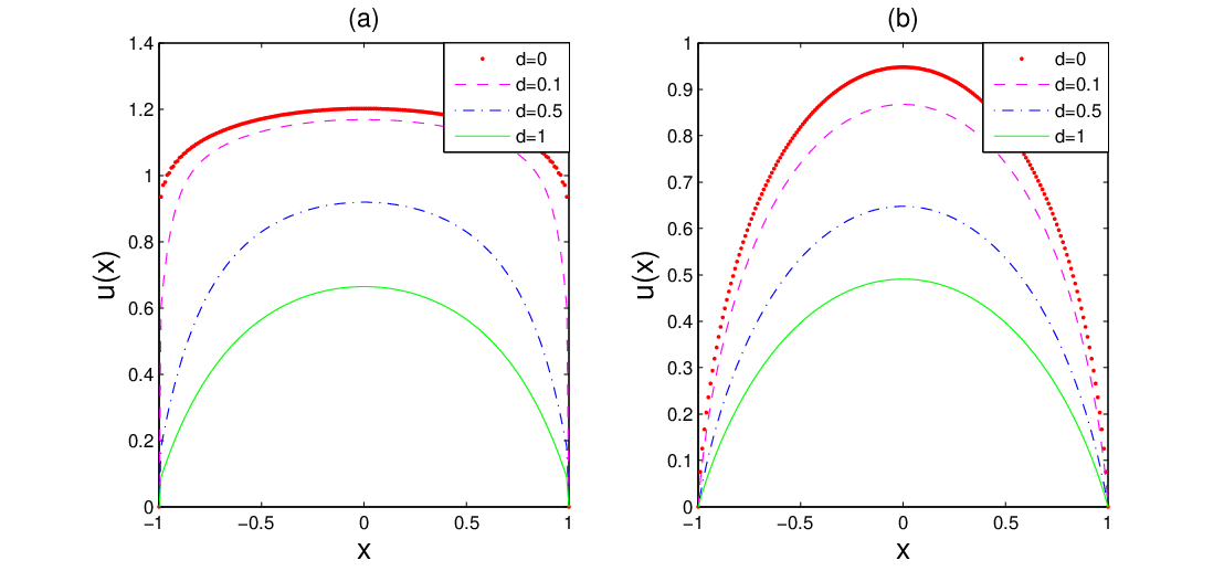
Having discussed the dependence of the mean exit times on the value of in the Lévy motion defined in the beginning of Sec. 3, we examine the effect of Gaussian noise on the profile of the mean exit time as a function of the location of the starting point . We vary the values of the diffusion coefficient and the parameter in Lévy measure independently. Thus, in the SDE, as defined by the generator in (8), is different than the traditional Lévy motion where the diffusion coefficient and the coefficient in Lévy measure are changed in tandem.
Consider the Lévy motion driven by O-U potential and the symmetric domain . Figure 9 shows the numerical results of the mean exit times with for different amount of Gaussian noises . For small values of (), such as as shown in Fig. 9(a), the mean exit time shapes as function of the starting point change dramatically as the amount of Gaussian noises increases. For small amount of Gaussian noises, the mean exit time profile is flat in the middle of the domain and drops to zero quickly near the boundary points; for large amount of Gaussian noises, the mean exit time profile become more parabla-like as shown in the graph for .
It is worth pointing out that the mean first exit time is discontinuous at the boundary in the case of pure non-Gaussian noise and , i.e., the limits are nonzero while . As mentioned in previous section, we have to use an one-sided difference scheme near the boundary to avoid numerically differentiating across discontinuities. From our numerical simulations for other values of and domain sizes (not shown here), we find that the mean exit time driven by O-U potential with ”pure” -stable jump only and would be discontinuous at the boundary of the domain. Recall that, in the absence of deterministic driving force () and Gaussian noise (), the mean exit time profile given in (21) become more ”discontinuous” at the boundary as (more precisely, the derivative of goes to infinity faster near the boundary for smaller values of ). Our numerical results show that adding O-U potential would cause the mean exit times be discontinuous at the boundary of the domain for all values of in and any domain size.
For large values of (), such as as shown in Fig. 9(a), the mean exit time shapes are similar to the parabolic shape as in the pure Gaussian noise case. Clearly, as the amount of Gaussian noises increases keeping other factors fixed, the mean exit times decreases. As shown in the figure, the mean exit time is continuous at the boundary even in the absence of Gaussian noise (). From the numerical simulations (not shown here), we also find that the mean exit times are continuous at the boundary for .

Next, we look at the effect of non-Gaussian noises by changing the parameter while keeping , and . It is obvious from the numerical results shown in Fig. 10 that the mean exit times decreases when the amount of non-Gaussian noises increases for all values of in . Due to the presence of significant Gaussian noises (), the shapes of the mean exit times are parabola-like for all parameter values shown in the figure. Keeping other parameters fixed, the effect of non-Gaussian noises on mean exit time is stronger when is larger. It is consistent with the previous result shown in Fig. 7(a) that, for small domains, the mean exit times decreases as increases.
5.4 Escape probability
In this section, we simulate the escape probability described by (9). In particular, for the special case of and , Eq. (9) becomes
| (28) |
for . The conditions for the escape probability outside the domain are for and for .

First, we verify our numerical schemes by comparing with the analytical result of the escape probability for the symmetric -stable case (, , ) with and [5]
| (29) |
As shown in Fig. 11(a) and (b), the numerical results match with the analytical results given in Eq. (29). Due to the symmetry of the process and the domains, the escape probability takes the value of one-half when the starting point is the position of symmetry . The escape probability is symmetric with respect to the point , i.e.,
These remain true even we add Brownian noise and the O-U potential to the process.
Due to the symmetry, in the following discussion we focus on positive starting points in the domain, i.e., . Figure 11 shows that the probability for the process to escape to the right of the domain is smaller when the value of decreases. For a fixed positive , the escape probability is the largest in for the case of Gaussian noise only (), keeping other factors the same. This property is independent of the domain size or whether there exists a deterministic driving mechanism . For larger domain sizes, as shown in Fig. 11(b,d,f), the escape probability tends to the value of equal chance especially for small values of . By comparing Fig. 11(c) with Fig.11(a) or comparing Fig. 11(d) with Fig. 11(b), we find that the effect of O-U potential is reducing the escape probability for the same starting point . The escape probability for the Brownian noise () is no longer a straight line in the presence of O-U potential. Again, for , we find that the escape probability is discontinuous at the boundary of the domain when the SDE is driven by the O-U potential and ”pure” -stable symmetric process, as demonstrated by the graphs of in Fig. 11(c) and (d). Adding Gaussian noises () to the processes increases the chances of escape to the right, as shown in Fig. 11(e) and (f).

Next, we consider SDE (1) driven by the double-well potential . The corresponding deterministic dynamical system has two stable states located at while is an unstable steady state. The double-well potential is well-known and widely used in phase transition studies.
We investigate the likelihood of the stochastic process that starts within a bounded domain and escapes and lands in the right-half line compared with that of escaping to the left of the bounded domain. We consider the bounded domains that includes the left stable point and the escape-target domain containing the other stable point . When a process lands in , in absence of the noises, it will be driven to and stay at the stable point . In other words, we try to examine the effect of noises on the likelihood of the transition from one stable state to the other. Figure 12(a) shows the escape probability for , and , when the stochastic effects are given by -stable symmetric processes only ( and ). The escape probability deviates more from a straight line as decreases and it is smaller for smaller when starting from . On the contrast, the probability is larger for smaller when the starting point is close to the left boundary of the bounded domain. For the bigger domain shown in Fig.12(b), the likelihood of escape to the right is more than a half for most of the starting points and ; the probability stays close to a half for most of the starting points when . Note that, in the case of , the probability is discontinuous at the left boundary of the domain. As shown in Fig.12(c) and (d), the differences in escape probabilities among different values of become smaller when an amount of Gaussian noises is added (), but otherwise probabilities have the similar values and properties compared with those of .
6 Conclusion
In summary, we have developed an accurate numerical scheme for solving the mean first exit time and escape probability for SDEs with non-Gaussian Lévy motions. We have analyzed the numerical error due to the singular nature of the Lévy measure corresponding to jumps and accordingly, added a correction term to the numerical scheme. We have validated the numerical method by comparing with analytical and asymptotic solutions. For arbitrary deterministic driving force, we have also given asymptotic solutions of the mean exit time when the pure jump measure in the Lévy motion is small.
Using both analytical and numerical results, we find that the mean exit time depends strongly on the domain size and the value of in the stable Lévy jump measure. For example, for -stable Lévy motion, the mean exit time can help us decide which of the two competing factors in -stable Lévy motion, the jump frequency or the jump size, is dominant. The small jumps with high frequency, corresponding to Lévy motion with closer to , make it easier to exit the small domains. On the other hand, it is easier to exit large domains for -stable Lévy motion with closer to , which has the characteristics of the large jumps with low frequency. Another observation from the results is that, for smaller values of (), the mean exit time profiles are flat away from the boundary of the domain. This implies that the jump sizes of the processes are usually larger than the domain sizes, thus the mean exit times have small variations for different starting positions.
The probability for the process to escape to the right of the domain is smaller when the value of decreases. For a fixed positive , the escape probability is the largest in for the case of Gaussian noise only (), keeping other factors the same. This property is independent of the domain size or whether there exists a deterministic driving mechanism . The escape probability is shown to vary significantly with the underlying vector field.
The mean exit time and escape probability could become discontinuous at the boundary of the domain, when the process is subject to certain deterministic potential and the value of is in .
References
- [1] S. Albeverrio, B. Rüdiger and J. L. Wu, Invariant Measures and Symmetry Property of Lévy Type Operators,Potential Analysis,13, 147-168, 2000.
- [2] D. Applebaum, Lévy Processes and Stochastic Calculus. Cambridge University Press, Cambridge, UK, 2004.
- [3] L. Arnold, Random Dynamical Systems. Springer-Verlag, New York, 1998.
- [4] J. Bertoin, Lévy Processes, Cambridge University Press, Cambridge, U.K., 1998.
- [5] R. M. Blumenthal, R. K. Getoor and D. B. Ray, On the distribution of first hits for the symmetric stable processes. Trans. Amer. Math. Soc. 99 (1961), 540-554.
- [6] J. Brannan, J. Duan and V. Ervin, Escape Probability, Mean Residence Time and Geophysical Fluid Particle Dynamics, Physica D 133 (1999), 23-33.
- [7] J. Brannan, J. Duan and V. Ervin, Escape probability and mean residence time in random flows with unsteady drift. Mathematical Problems in Engineering Volume 7 (2001), Issue 1, Pages 55-65. doi:10.1155/S1024123X01001521
- [8] Z. Chen, P. Kim and R. Song, Heat kernel estimates for Dirichlet fractional Laplacian. J. European Math. Soc. 12 (2010), 1307-1329.
- [9] D. del-Castillo-Negrete, V.Yu. Gonchar, A.V. Chechkin, Fluctuation-driven directed transport in the presence of Lévy flights. Physica A, 27 6693-6704. (2008).
- [10] D. del-Castillo-Negrete, Non-diffusive, non-local transport in fluids and plasmas. Nonlin. Processes Geophys., 17, 795-807, (2010).
- [11] P. D. Ditlevsen, Observation of stable noise induced millennial climate changes from an ice record. Geophys. Res. Lett. 26 (1999), 1441-1444.
- [12] M. I. Freidlin and A. D. Wentzell, Random Perturbations of Dynamical Systems, 2nd edition, Springer-Verlag, 1998.
- [13] R. K. Getoor, First passage times for symmetric stable processes in space. Trans. Amer. Math. Soc. 101, 75¨C90 (1961).
- [14] V. V. Godovanchuk, Asymptotic probabilities of large deviations due to large jumps of a Markov process, Theory of probability and its applications, Volume XXVI, 1981, p. 314-327.
- [15] P. Imkeller and I. Pavlyukevich, First exit time of SDEs driven by stable Lévy processes. Stoch. Proc. Appl. 116 (2006), 611-642.
- [16] P. Imkeller, I. Pavlyukevich and T. Wetzel, First exit times for Lévy-driven diffusions with exponentially light jumps. Ann. Probab. Volume 37, Number 2 (2009), 530-564. arXiv:0711.0982.
- [17] H. Kunita, Stochastic differential equations based on Lévy processes and stochastic flows of diffeomorphisms. Real and stochastic analysis, 305–373, Trends Math., Birkhuser Boston, Boston, MA, 2004.
- [18] M. Liao, The Dirichlet problem of a discontinuous Markov process. Acta Math. Sinica (New Series) 5(1) (1989), 9-15.
- [19] T. Naeh, M. M. Klosek, B. J. Matkowsky and Z. Schuss, A direct approach to the exit problem, SIAM J. Appl. Math. 50 (1990), 595-627.
- [20] I. Navot, An extension of the Euler-Maclaurin summation formula to functions with branch singularity. J. Math. and Phys. 40 (1961), 271–276.
- [21] B. Oksendal, Applied Stochastic Control Of Jump Diffusions. Springer-Verlag, New York, 2005.
- [22] S. Peszat and J. Zabczyk, Stochastic Partial Differential Equations with Lévy Processes, Cambridge University Press, Cambridge, UK, 2007.
- [23] K.-I. Sato, Lévy Processes and Infinitely Divisible Distributions, Cambridge University Press, Cambridge, 1999.
- [24] D. Schertzer, M. Larcheveque, J. Duan, V. Yanovsky and S. Lovejoy, Fractional Fokker–Planck equation for nonlinear stochastic differential equations driven by non-Gaussian Lévy stable noises. J. Math. Phys., 42 (2001), 200-212.
- [25] Z. Schuss, Theory and Applications of Stochastic Differential Equations, Wiley Sons, New York, 1980.
- [26] M. F. Shlesinger, G. M. Zaslavsky and U. Frisch, Lévy Flights and Related Topics in Physics (Lecture Notes in Physics, 450. Springer-Verlag, Berlin, 1995).
- [27] R. Song, Probabilistic approach to the Dirichlet problem of perturbed stable processes. Probab. Theory Related Fields, 95(3) (1993), 371-389.
- [28] W. A. Woyczynski, Lévy processes in the physical sciences. In Lévy Processes: Theory and Applications, O. E. Barndorff-Nielsen, T. Mikosch and S. I. Resnick (Eds.), 241-266, Birkhäuser, Boston, 2001.
- [29] Z. Yang and J. Duan, An intermediate regime for exit phenomena driven by non-Gaussian Lévy noises. Stochastics and Dynamics, Vol.8, No.3, 583-591, 2008.