A Cosmology Forecast Toolkit – CosmoLib

Let us start discussing the background solutions. We consider a flat FRW metric $ds^{2}=a^{2}(\tau)(-d\tau^{2}+dx^{i}dx^{i})$, where $a$ is the scale factor and $\tau$ is the conformal time. The normalization of $a$ is arbitrary. We normalize it such that $a=1$ today. CosmoLib uses the e-fold number $N\equiv\ln a$ as the time variable. The physical Hubble expansion rate is defined as $H\equiv\frac{da/d\tau}{a^{2}}$. Its present value is denoted by $H_{0}\equiv 100h{\,\rm km\,}{\rm s}^{-1}{\,\rm Mpc}^{-1}$.

We assume a universe with cold dark matter (labeled with a subscript $c$), dark energy (labeled with a subscript $\Lambda$), baryons (labeled with a subscriber $b$), radiation (labeled with a subscript $\gamma$), and 3 species of massless neutrinos (labeled with a subscript $\nu$). For a component $X$ ($X=b,c,\gamma,\nu,\Lambda$) the background density is denoted as $\rho_{X}$, and the background pressure $p_{X}$. The present-day fractional energy density is written as $\Omega_{X0}$ . Dark energy is assumed to be a perfect fluid with known equation of state (pressure to density ratio) $w(a)$ and a constant sound speed $c_{s,\Lambda}^{2}$ in its rest frame. The users can either choose $w(a)$ from a list of build-in models or define their own $w(a)$ functions. The build-in models of $w(a)$ include the cosmological constant model $w(a)=-1$ [59], a constant EOS $w(a)=w_{0}$, a linear function $w(a)=w_{0}+w_{a}(1-a)$ [60, 61], and a general three-parameter parametrization for the minimally coupled quintessence/phantom models [62].

For a given $w(a)$ the background solutions are

We will also use the derived quantities $\Omega_{X}(a)\equiv\rho_{X}/(3H^{2}M_{p}^{2})$ ($X=b,c,\gamma,\nu,\Lambda$), $R\equiv(3\rho_{b})/(4\rho_{\gamma})$, and

The conformal time $\tau$ can be related to the scale factor $a=e^{N}$ via

The electron number density $n_{e}(a)$ is obtained using RecFast version 1.5 [63, 64], which has been incorporated into CosmoLib. We denote the differential optical depth (increment of optical depth per $dN$) as

where $\sigma_{T}=6.652\times 10^{-25}{\rm cm}^{2}$ is the Thomson scattering cross section. The baryon sound speed $c_{s,b}^{2}(a)$ is obtained by solving the differential equations (68-69) in Ref. [40].

With these background solutions in hand, now we can write down the governing equations for scalar perturbations.

The metric in the (generalized) Newtonian gauge can be written as

where $\partial_{i}\omega_{i}=0$, $h_{ii}=0$ and $\partial_{i}h_{ij}=0$. The vector perturbation $\omega_{i}$ decays in an expanding universe and hence it is set to zero in CosmoLib. The tensor perturbation $h_{ij}$ is gauge-invariant and its governing equations are identical in all gauges. Thus, we will only focus on the scalar perturbation equations that in CosmoLib differ from those in many other Boltzmann codes.

The linear-order relative density perturbation of $X$ is denoted by $\delta_{X}\equiv\delta\rho_{X}/\rho_{X}$, and the linear-order velocity $\upsilon_{X}$. Unless otherwise specified, $\delta_{X}$ and $\upsilon_{X}$ are all defined in Fourier space, that are functions of $\tau$ and the wave vector $\mathbf{k}$.

The radiation relative temperature fluctuation $\Delta T/T$ from direction $\mathbf{n}$ seen by an observer at position $\mathbf{x}$ is expanded as [17]

where $Y_{\ell}^{m}$ are the spherical harmonic functions. Note that the moments $\Theta_{\gamma}(\ell,m)$ are functions of the wavenumber $\mathbf{k}$ and the conformal time $\tau$. The energy density fluctuation and velocity of photons are related to the moments $\ell=0$ and $\ell=1$ via

The neutrino moments $\Theta_{\nu}(\ell,m)$ are defined in the same way, by replacing the subscript $\gamma$ with $\nu$.

For the polarization of radiation, the Stokes parameters $Q,U$ are expanded using the spin-$2$ harmonics ${}_{\pm 2}Y_{\ell}^{m}$ [17]

where $E(\ell,m)$ and $B(\ell,m)$ are functions of the wave vector $\mathbf{k}$ and conformal time.

The linear-order Fourier modes are decoupled. The Fourier-space variables to be evolved are $\Psi$, $\Psi_{N}\equiv d\Psi/dN$, $\delta_{b}$, $\upsilon_{b}$, $\delta_{c}$, $\upsilon_{c}$, $\delta_{\Lambda}$, $\theta_{\Lambda}\equiv(1+w)\upsilon_{\Lambda}$, $\Theta_{\gamma}(\ell,0)$ ($\ell$ = $0$, $1$, $2$, …, $\ell_{\max,\gamma}$), $\Theta_{\nu}(\ell,0)$ ($\ell$ = $0$, $1$, $2$, …, $\ell_{\max,\nu}$), $E(\ell,0)$ ($\ell$ = $2$, …, $\ell_{\max,E}$). The truncations $\ell_{\max,\gamma}$, $\ell_{\max,\nu}$ and $\ell_{\max,E}$ are adjustable integers. In CosmoLib their default values are taken to be $14$, $12$, $14$, respectively. Without loss of generality we choose the azimuthal direction (the $z$-axis direction that is used to define $Y_{\ell,m}(\mathbf{n})$) to be parallel to $\mathbf{k}$.

The gravitational potential $\Phi$ can be obtained from the Einstein equations [65, 40, 17]

where we have introduced the reduced wavenumber

Note that $k_{H},\Omega_{\gamma},\Omega_{\nu}$ are functions of time. We do not treat $\Phi$ as an independent-variable. Instead we view it as a function of the variables $\Psi$, $\Theta_{\gamma}(2,0)$ and $\Theta_{\nu}(2,0)$.

The close set of first-order differential equations including all the truncation schemes is:

In the radiation and neutrino hierarchy equations (18-29) we have used the Clebsch-Gordan coefficients $K_{l,m,s}$, which are defined as [17]

These equations are already written in the form that can be directly implemented into a generic first-order ordinary-differential-equation (ODE) solver. For a derivation of these equations, see Refs. [65, 40, 17, 66]. (The change of time variable from $\tau$ to $N$ can be done straightforwardly using $d/d\tau=aHd/dN$.) The initial conditions can be found in Ref. [40]. For the tight-coupling approximation we follow Ref. [67], where the obvious typos in Eqs. (15-16) has been fixed. Since these treatments are identical to the original source, we do not repeat the discussion here. The interested readers are referred to these references for the governing equations and their derivation.

CosmoLib allows the user-input $w(a)$ to be a phantom-crossing function, that is a function crossing the line $w=-1$. In this case we force $d\delta_{\Lambda}/dN$ and $d\theta_{\Lambda}/dN$ to be zero around the proximity of the phantom crossing. This is an approximation. Exact treatment requires input of at least one more degree of freedom [68, 69, 70], which cannot be implemented in a generic code. In Ref. [66] the reader can find an alternative treatment that works better for multiple scalar field models.

Equation (30) is the key equation that guarantees the numerical stability of the code (even for isocurvature initial conditions). It is obtained by subtracting the $ii$ components of the perturbed Einstein equations (pressure perturbations) from the $00$ component (density perturbations). This particular combination of the Einstein equations has been applied in the numerical code CMBquick [50, 71], which assumes that dark energy is a cosmological constant and ignores the baryon sound speed. Eq. (30) is a generalized version that includes dark energy perturbations and a nonzero baryon sound speed.

We can use the energy constraint ($00$ component of the perturbed Einstein equations, that is $\delta G_{00}=\delta T_{00}$) and the momentum constraint ($0i$-component of the perturbed Einstein equations, that is $\delta G_{0i}=\delta T_{0i}$) to estimate the numerical error of the code. As shown in shown in Figure 1, the relative errors are $\lesssim 10^{-4}$ for a wide range of scales and different initial conditions.

Optionally CosmoLib can compute the CMB angular power spectrum for each multipole $\ell$ by brute force, i.e., without interpolation. The angular spectrum for the temperature anisotropies is given by

where $\Delta_{\ell}^{k}$ is the temperature transfer function given by the line-of-sight integration

where $j_{\ell}$ is the spherical Bessel function and $\tau_{0}$ is $\tau$ at redshift zero. The source $S(k,\tau)$ can be computed from the perturbations $\Psi$, $\Phi$, $\delta_{X}$, $\upsilon_{X}$ ($X=c$, $b$, $\Lambda$, $\gamma$, $\nu$), $\Theta_{\gamma}(2,0)$ and $\Theta_{\nu}(2,0)$ [12, 17]. In Ref. [17] the line-of-sight integration involves the functions $j_{\ell}$, $j^{\prime}_{\ell}$ and $j_{\ell}^{\prime\prime}$. As shown in Ref. [12], however, the dependence on $j_{\ell}^{\prime}$ and $j_{\ell}^{\prime\prime}$ can be eliminated by integrating by part. (We have corrected the obvious typos in eq. (12b) in Ref. [12].)

Since $\Delta_{\ell}^{k}$ is evaluated numerically and it typically oscillates quickly, its sampling is time consuming. Indeed, in modern fast CMB codes – such as CAMB, CLASS, CMBEASY – the integral (32) is computed by sampling $\Delta_{\ell}^{k}$ using a step size in $k$ that can be typically much larger than the oscillation period in $\Delta_{\ell}^{k}$. For instance, in Fig. 2 we show an example of $\Delta_{\ell}^{k}$ for a fixed $\ell=300$. A typical sampling scheme is shown by the red solid triangles in the upper-right panel, which zooms-in part of the figure. According to Parseval’s theorem, if $\mathcal{P}_{s}(\ln k)$ is a smooth function, such sparse sampling of $\Delta_{\ell}^{k}$ is enough.

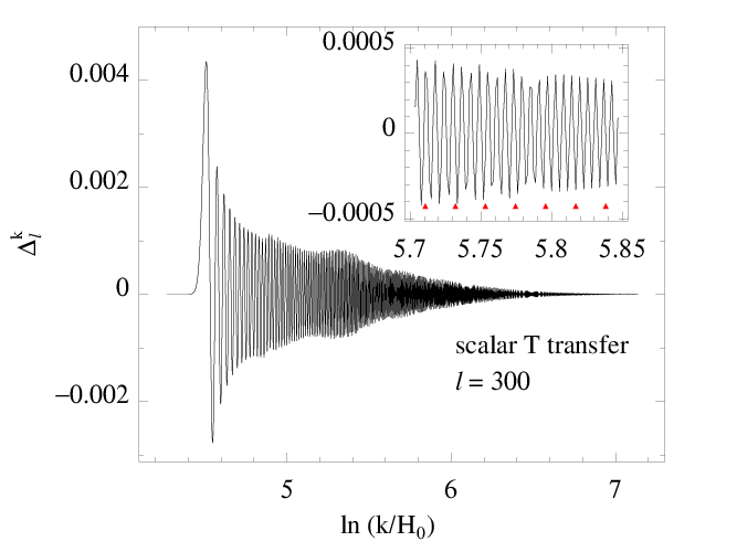
However, when $\mathcal{P}_{s}(k)$ has local sharp features, the minimum sampling distance should be determined by the larger between the typical relative width (the width measured in $\ln k$) of the oscillations in $\Delta_{\ell}^{k}$ and $\delta\ln k$, the typical relative width of the features in $\mathcal{P}_{s}(k)$. The former is about $10^{-4}-10^{-3}$, while the latter is model-dependent. For instance, if our goal is to sample features with width $\delta\ln k\sim 10^{-3}$, the required sampling frequency is typically $\sim 20$ to $100$ times higher than that used for a smooth $\mathcal{P}_{s}(k)$. Furthermore, as we wish to compute the $C_{\ell}$’s for each $\ell$ rather than interpolating it over few tens of $\ell$’s, the total time consumption will be again multiplied by a factor of $\sim 10-50$. The naively estimated total time consumption is hence $\sim 10^{3}$ times more than that in the smooth-$\mathcal{P}_{s}(k)$ case. A final complication is due to the fact that, if all the transfer functions and the precomputed $j_{\ell}(x)$ tables are to be stored, one has also to face a memory barrier that cannot be easily bypassed. For these reasons, simply increasing the $\ell$ and $k$ resolution in standard codes such as CAMB, CLASS or CMBEASY, will not be efficient enough for the purpose of scanning the whole parameter space.

The algorithm can be significantly improved, however, if we notice that the output $S(k,\tau)$ from the Boltzmann code is a 2D matrix in $k$-$\tau$ space. If $j_{\ell}\left[k(\tau_{0}-\tau)\right]$ is also a precomputed 2D matrix with the same structure, the integration (33) can be obtained by taking the inner product of the two matrices. Modern Fortran90 compilers can optimize such operation and make the computation much faster. The difficulty, however, is that the $j_{\ell}\left[k(\tau_{0}-\tau)\right]$ matrices for all $\ell$’s will occupy too much memory (can be up to a few tens of Giga bytes in the worst scenario). Our solution is then to only store the matrices for two neighboring $\ell$’s and update them using the recurrence relation of spherical Bessel functions.

Let us describe our strategy. We first compute two neighboring $C_{\ell}$’s by brute force. Two matrices of spherical Bessel functions $j_{\ell+1}[k(\tau_{0}-\tau)]$ and $j_{\ell}[k(\tau_{0}-\tau)]$ are stored in the memory for each $(k,\tau)$ indices. Then we compute $C_{\ell-1}$. To do that, we update the $j_{\ell+1}$ matrix to the $j_{\ell-1}$ matrix using the recurrence relation

Again, using $j_{\ell}$ and $j_{\ell-1}$ we then calculate $j_{\ell-2}$ and hence $C_{\ell-2}$. This downward iteration is very stable for a few tens of steps, after which we need to recompute another couple of neighboring $C_{\ell}$’s and iterate downward again.

The initial neighboring $j_{\ell}$’s are calculated using precomputed 25-th order Chebyshev fitting formulas. (For the rapidly oscillating part at $x\gg l$, the phase and amplitude of oscillations are fitted using Chebyshev polynomials.) Chebyshev fitting is slightly slower than the cubic-spline fitting used in other publicly available CMB codes, but it is more memory-efficient and more accurate – it has an accuracy of $\sim 10^{-8}$ – and allows more downward iterative steps. Finally, note that the algorithm proposed here is more efficient both CPU-wise and memory-wise, enhancing the speed of $\ell$-by-$\ell$ computation of $C_{\ell}$’s by a factor of $\sim 10$ to $30$.

For CMB lensing we use the power spectrum approach as described in Refs. [72, 73].

The trivial comparison between CosmoLib and CAMB for smooth-$\mathcal{P}_{s}$ models can be found in the online documentation at http://www.cita.utoronto.ca/~zqhuang/CosmoLib. Here we focus on the enhanced CMB integrator that does not assume the smoothness in $\mathcal{P}_{s}(k)$. Since this feature is not available in other CMB codes, direct numerical comparison is not possible when there is very sharp features in $\mathcal{P}_{s}$. Thus, we need to study a model in which we have some theoretical insights. An ideal candidate is the axion monodromy inflation model, where the primordial power spectrum displays sinusoidal oscillations superimposed to a smooth power spectrum. It can be written as [38]

where $A_{s}$ and $n_{s}$ are the amplitude and tilt, respectively. The parameter $\delta\ln k$ describes the width of the oscillations in $\mathcal{P}_{s}(k)$, while $\delta n_{s}$ gives their relative amplitude. The pivot scale $k_{*}$ is chosen to be $0.05{\rm Mpc}^{-1}$ in our computation.

We compute the CMB temperature power spectrum using the enhanced CMB integrator in CosmoLib and compare the results to the smooth-$\mathcal{P}_{s}(k)$ case. The relative difference between the non-smooth (for a series of $\delta\ln k$) and the smooth model is shown in Figure 3. For $\delta\ln k=0.1$ and $\delta\ln k=0.03$ we compare the results to CAMB output (both with lensing) and find good agreement. The CAMB outputs are obtained by a straightforward modification of CAMB, i.e., increasing the $\ell$ sampling frequency in the input file and increasing the $k$ sampling frequency in the source code. For $\delta\ln k\lesssim 0.01$ the simple modification of CAMB fails due to insufficient memory to store the transfer functions.

For $\delta\ln k\ll 1$, the amplitude of oscillations in the CMB angular power spectrum (right-hand panels) is smaller than that in $\mathcal{P}_{s}(k)$ (left-hand panels). This suppression is generic when a 3D power spectrum is projected to a 2D one, even though in the CMB case it is further complicated by the finite duration of recombination and the recombination physics [74]. As shown in [58], when the frequency of oscillations is constant in $\ln k$, such as in eq. (35), the relative suppression is given by $\sim\sqrt{\delta\ln k}$, as confirmed by the examples shown in Figure 3. Moreover, for $\delta\ln k\lesssim 0.01$, in addition to the projection effect, CMB lensing also significantly smears out the oscillations in $C_{\ell}$ at high $\ell\gtrsim 2000$. While for $\delta\ln k=0.1$, the lensing smearing effect is almost negligible. See [74, 75] for more detailed discussions about the lensing smearing effect. Finally, note that, although the oscillations in $C_{\ell}$ are damped, they maintain the same relative width of those of the left-hand panels, i.e., $\delta\ln\ell=\delta\ln k$ where $\ell\gtrsim(\delta\ln k)^{-1}$. At low $\ell$ where $\ell\lesssim 1/\delta\ln k$ the oscillations in $k$ space disappear in $\ell$ space due to the discreteness of $\ell$.

This discussion shows that the enhanced CMB integrator can accurately compute the oscillations in CMB to $\Delta C_{\ell}/C_{\ell}\lesssim 10^{-3}$. This does not mean, however, that the total $C_{\ell}$ is accurate to $10^{-3}$. The $C_{\ell}$ power spectrum can be systematically biased at subpercent level due to, e.g., recombination uncertainties [76]. Understanding and eliminating these theoretical errors is important if we want to extract generic features in $\mathcal{P}_{s}(k)$ with $10^{-3}$ accuracy. On the other hand, if we are only interested in a model predicting a specific feature in $C_{\ell}$ that cannot be mimicked by other effects, we can focus only on the relative difference in $C_{\ell}$.