Homoclinic Orbits of the FitzHugh-Nagumo Equation: The Singular-Limit
Abstract
The FitzHugh-Nagumo equation has been investigated with a wide array of different methods in the last three decades. Recently a version of the equations with an applied current was analyzed by Champneys, Kirk, Knobloch, Oldeman and Sneyd [5] using numerical continuation methods. They obtained a complicated bifurcation diagram in parameter space featuring a C-shaped curve of homoclinic bifurcations and a U-shaped curve of Hopf bifurcations. We use techniques from multiple time-scale dynamics to understand the structures of this bifurcation diagram based on geometric singular perturbation analysis of the FitzHugh-Nagumo equation. Numerical and analytical techniques show that if the ratio of the time-scales in the FitzHugh-Nagumo equation tends to zero, then our singular limit analysis correctly represents the observed CU-structure. Geometric insight from the analysis can even be used to compute bifurcation curves which are inaccessible via continuation methods. The results of our analysis are summarized in a singular bifurcation diagram.
1 Introduction
1.1 Fast-Slow Systems
Fast-slow systems of ordinary differential equations (ODEs) have the general form:
| (1) | |||||
where , and represents the ratio of time scales. The functions and are assumed to be sufficiently smooth. In the singular limit the vector field (1) becomes a differential-algebraic equation. The algebraic constraint defines the critical manifold . Where is nonsingular, the implicit function theorem implies that there exists a map parametrizing as a graph. This yields the implicitly defined vector field on called the slow flow.
We can change (1) to the fast time scale and let to obtain the second possible singular limit system
| (2) | |||||
We call the vector field (2) parametrized by the slow variables the fast subsystem or the layer equations. The central idea of singular perturbation analysis is to use information about the fast subsystem and the slow flow to understand the full system (1). One of the main tools is Fenichel’s Theorem (see [16, 17, 18, 19]). It states that for every sufficiently small and normally hyperbolic there exists a family of invariant manifolds for the flow (1). The manifolds are at a distance from and the flows on them converge to the slow flow on as . Points where is singular are referred to as fold points11
1
The projection of onto the coordinates may have more degenerate singularities than fold singularities at some of these points..
Beyond Fenichel’s Theorem many other techniques have been developed. More detailed introductions and results can be found in [12, 34, 24] from a geometric viewpoint. Asymptotic methods are developed in [42, 23] whereas ideas from nonstandard analysis are introduced in [8]. While the theory is well developed for two-dimensional fast-slow systems, higher-dimensional fast-slow systems are an active area of current research. In the following we shall focus on the FitzHugh-Nagumo equation viewed as a three-dimensional fast-slow system.
1.2 The FitzHugh-Nagumo Equation
The FitzHugh-Nagumo equation is a simplification of the Hodgin-Huxley model for an electric potential of a nerve axon [30]. The first version was developed by FitzHugh [20] and is a two-dimensional system of ODEs:
| (3) | |||||
A detailed summary of the bifurcations of (3) can be found in [44]. Nagumo et al. [43] studied a related equation that adds a diffusion term for the conduction process of action potentials along nerves:
| (4) |
where and and are parameters. A good introduction to the derivation and problems associated with (4) can be found in [28]. Suppose we assume a traveling wave solution to (4) and set and , where represents the wave speed. By the chain rule we get , and . Set and substitute into (4) to obtain the system:
| (5) | |||||
System (5) is the FitzHugh-Nagumo equation studied in this paper. Observe that a homoclinic orbit of (5) corresponds to a traveling pulse solution of (4). These solutions are of special importance in neuroscience [28] and have been analyzed using several different methods. For example, it has been proved that (5) admits homoclinic orbits [29, 4] for small wave speeds (“slow waves”) and large wave speeds (“fast waves”). Fast waves are stable [33] and slow waves are unstable [21]. It has been shown that double-pulse homoclinic orbits [15] are possible. If (5) has two equilibrium points and heteroclinic connections exist, bifurcation from a twisted double heteroclinic connection implies the existence of multi-pulse traveling front and back waves [6]. These results are based on the assumption of certain parameter ranges for which we refer to the original papers. Geometric singular perturbation theory has been used successfully to analyze (5). In [32] the fast pulse is constructed using the exchange lemma [35, 31, 3]. The exchange lemma has also been used to prove the existence of a codimension two connection between fast and slow waves in ()-parameter space [38]. An extension of Fenichel’s theorem and Melnikov’s method can be employed to prove the existence of heteroclinic connections for parameter regimes of (5) with two fixed points [45]. The general theory of relaxation oscillations in fast-slow systems applies to (5) (see e.g. [42, 26]) as does - at least partially - the theory of canards (see e.g. [46, 9, 11, 39]).
The equations (5) have been analyzed numerically by Champneys, Kirk, Knobloch, Oldeman and Sneyd [5] using the numerical bifurcation software AUTO [13, 14]. They considered the following parameter values:
We shall fix those values to allow comparison of our results with theirs. Hence we also write . Changing from the fast time to the slow time and relabeling variables , and we get:
| (6) | |||||
From now on we refer to (6) as “the” FitzHugh-Nagumo equation. Investigating bifurcations in the () parameter space one finds C-shaped curves of homoclinic orbits and a U-shaped curve of Hopf bifurcations; see Figure 1. Only part of the bifurcation diagram is shown in Figure 1. There is another curve of homoclinic bifurcations on the right side of the U-shaped Hopf curve. Since (6) has the symmetry
| (7) |
we shall examine only the left side of the U-curve. The homoclinic C-curve is difficult to compute numerically by continuation methods using AUTO [13, 14] or MatCont [22]. The computations seem infeasible for small values of . Furthermore multi-pulse homoclinic orbits can exist very close to single pulse ones and distinguishing between them must necessarily encounter problems with numerical precision [5]. The Hopf curve and the bifurcations of limit cycles shown in Figure 1 have been computed using MatCont. The curve of homoclinic bifurcations has been computed by a new method to be described in Section 3.2.

Since the bifurcation structure shown in Figure 1 was also observed for other excitable systems, Champneys et al. [5] introduced the term CU-system. Bifurcation analysis from the viewpoint of geometric singular perturbation theory has been carried out for examples with one fast and two slow variables [27, 2, 25, 41]. Since the FitzHugh-Nagumo equation has one slow and two fast variables, the situation is quite different and new techniques have to be developed. Our main goal is to show that many features of the complicated 2-parameter bifurcation diagram shown in Figure 1 can be derived with a combination of techniques from singular perturbation theory, bifurcation theory and robust numerical methods. We accurately locate where the system has canards and determine the orbit structure of the homoclinic and periodic orbits associated to the C-shaped and U-shaped bifurcation curves, without computing the canards themselves. We demonstrate that the basic CU-structure of the system can be computed with elementary methods that do not use continuation methods based on collocation. The analysis of the slow and fast subsystems yields a “singular bifurcation diagram” to which the basic CU structure in Figure 1 converges as .
Remark: We have also investigated the termination mechanism of the C-shaped homoclinic curve described in [5]. Champneys et al. observed that the homoclinic curve does not reach the U-shaped Hopf curve but turns around and folds back close to itself. We compute accurate approximations of the homoclinic orbits for smaller values than seems possible with AUTO in this region. One aspect of our analysis is a new algorithm for computing invariant slow manifolds of saddle type in the full system. This work will be described elsewhere.
2 The Singular Limit
The first step in our analysis is to investigate the slow and fast subsystems separately. Let in (6); this yields two algebraic constraints that define the critical manifold:
Therefore is a cubic curve in the coordinate plane . The parameter moves the cubic up and down inside this plane. The critical points of the cubic are solutions of and are given by:
The points are fold points with since is a cubic polynomial with distinct critical points. The fold points divide into three segments
We denote the associated slow manifolds by , and . There are two possibilities to obtain the slow flow. One way is to solve for and substitute the result into the equation . Alternatively differentiating implicitly with respect to yields and therefore
| (8) |
One can view this as a projection of the slow flow, which is constrained to the critical manifold in , onto the -axis. Observe that the slow flow is singular at the fold points. Direct computation shows that the fixed point problem has only a single real solution. This implies that the critical manifold intersects the diagonal only in a single point which is the unique equilibrium of the slow flow (8). Observe that is also the unique equilibrium of the full system (6) and depends on . Increasing moves the equilibrium from left to right on the critical manifold. The easiest practical way to determine the direction of the slow flow on is to look at the sign of . The situation is illustrated in Figure 2.

2.1 The Slow Flow
We are interested in the bifurcations of the slow flow depending on the parameter . The bifurcations occur when passes through the fold points. The values of can simply be found by solving the equations and simultaneously. The result is:
where the subscripts indicate the fold point at which each equilibrium is located.
The singular time-rescaling of the slow flow yields the desingularized slow flow
| (9) |
Time is reversed by this rescaling on and since and is negative on these branches. The desingularized slow flow (9) is smooth and has no bifurcations as is varied.
2.2 The Fast Subsystem
The key component of the fast-slow analysis for the FitzHugh-Nagumo equation is the two-dimensional fast subsystem
| (10) |
where , are parameters and is fixed. Since and have the same effect as bifurcation parameters we set . We consider several fixed y-values and the effect of varying (cf. Section 3.2) in each case. There are either one, two or three equilibrium points for (10). Equilibrium points satisfy and lie on the critical manifold, i.e. we have to solve
| (11) |
for . We find that there are three equilibria for approximately , two equilibria on the boundary of this interval and one equilibrium otherwise. The Jacobian of (10) at an equilibrium is
Direct calculation yields that for the single equilibrium is a saddle. In the case of three equilibria, we have a source that lies between two saddles. Note that this also describes the stability of the three branches of the critical manifold , and . For the matrix is singular of rank 1 if and only if which occurs for the fold points . Hence the equilibria of the fast subsystem undergo a fold (or saddle-node) bifurcation once they approach the fold points of the critical manifold. This happens for parameter values and . Note that by symmetry we can reduce to studying a single fold point. In the limit (corresponding to the case of a “standing wave”) the saddle-node bifurcation point becomes more degenerate with nilpotent.
Our next goal is to investigate global bifurcations of (10); we start with homoclinic orbits. For it is easy to see that (10) is a Hamiltonian system:
| (12) |
with Hamiltonian function
| (13) |
We will use this Hamiltonian formulation later on to describe the geometry of homoclinic orbits for slow wave speeds. Assume that is chosen so that
(12) has a homoclinic orbit . We are interested in perturbations with and note that in this case the divergence of (10) is . Hence the vector field is area expanding everywhere. The homoclinic orbit breaks for and no periodic orbits are created. Note that this scenario does not apply to the full three-dimensional system as the equilibrium has a pair of complex conjugate eigenvalues so that a Shilnikov scenario can occur. This illustrates that the singular limit can be used to help locate homoclinic orbits of the full system, but that some characteristics of these orbits change in the singular limit.
We are interested next in finding curves in -parameter space that represent heteroclinic connections of the fast subsystem. The main motivation is the decomposition of trajectories in the full system into slow and fast segments. Concatenating fast heteroclinic segments and slow flow segments can yield homoclinic orbits of the full system [28, 4, 32, 38]. We describe a numerical strategy to detect heteroclinic connections in the fast subsystem and continue them in parameter space. Suppose that so that (10) has three hyperbolic equilibrium points , and . We denote by the unstable and by the stable manifold of . The same notation is also used for and tangent spaces to and are denoted by and . Recall that is a source and shall not be of interest to us for now. Define the cross section by
We use forward integration of initial conditions in and backward integration of initial conditions in to obtain trajectories and respectively. We calculate their intersection with and define
We compute the functions and for different parameter values of numerically. Heteroclinic connections occur at zeros of the function
Once we find a parameter pair such that , these parameters can be continued along a curve of heteroclinic connections in parameter space by solving the root-finding problem for either or fixed and small. We use this method later for different fixed values of to compute heteroclinic connections in the fast subsystem in parameter space. The results of these computations are illustrated in Figure 3. There are two distinct branches in Figure 3. The branches are asymptotic to and and approximately form a “”. From Figure 3 we conjecture that there exists a double heteroclinic orbit for .

Remarks: If we fix our initial change of variable becomes and our results for heteroclinic connections are for the FitzHugh-Nagumo equation without an applied current. In this situation it has been shown that the heteroclinic connections of the fast subsystem can be used to prove the existence of homoclinic orbits to the unique saddle equilibrium (cf. [32]). Note that the existence of the heteroclinics in the fast subsystem was proved in a special case analytically [1] but Figure 3 is - to the best of our knowledge - the first explicit computation of where fast subsystem heteroclinics are located. The paper [36] develops a method for finding heteroclinic connections by the same basic approach we used, i.e. defining a codimension one hyperplane that separates equilibrium points.
Figure 3 suggests that there exists a double heteroclinic connection for . Observe that the Hamiltonian in our case is where the function is:
The solution curves of (12) are given by . The structure of the solution curves entails symmetry under reflection about the -axis. Suppose and recall that we denoted the two saddle points of (10) by and and that their location depends on . Therefore, we conclude that the two saddles and must have a heteroclinic connection if they lie on the same energy level, i.e. they satisfy . This equation can be solved numerically to very high accuracy.
Proposition 1.
The fast subsystem of the FitzHugh-Nagumo equation for has a double heteroclinic connection for . Given a particular value there exists a double heteroclinic connection for in the fast subsystem lying in the plane .
2.3 Two Slow Variables, One Fast Variable
From continuation of periodic orbits in the full system - to be described in Section 3.1 - we observe that near the U-shaped curve of Hopf bifurcations the -coordinate is a faster variable than . In particular, the small periodic orbits generated in the Hopf bifurcation lie almost in the plane . Hence to analyze this region we set to transform the FitzHugh-Nagumo equation (6) into a system with 2 slow and 1 fast variable:
| (14) | |||||
Note that (14) corresponds to the FitzHugh-Nagumo equation in the form (cf. (4)):
| (15) |
Therefore the transformation can be viewed as a rescaling of the diffusion strength by . We introduce a new independent small parameter and then let . This assumes that terms do not vanish in this limit, yielding the diffusion free system. Then the slow manifold of (14) is:
| (16) |
Proposition 2.
Remark: The reduction to equations (17)-(18) suggests that (14) is a three time-scale system. Note however that (14) is not given in the three time-scale form for and . The time-scale separation in (17)-(18) results from the singular dependence of the critical manifold ; see (16).
Proof.
Before we start with the analysis of (17) we note that detailed bifurcation calculations for (17) exist. For example, Rocsoreanu et al. [44] give a detailed overview on the FitzHugh equation (17) and collect many relevant references. Therefore we shall only state the relevant bifurcation results and focus on the fast-slow structure and canards. Equation (17) has a critical manifold given by which coincides with the critical manifold of the full FitzHugh-Nagumo system (6). Formally it is located in but we still denote it by . Recall that the fold points are located at
Also recall that the y-nullcline passes through the fold points at:
We easily find that supercritical Hopf bifurcations are located at the values
| (19) |
For the case we get and . The periodic orbits generated in the Hopf bifurcations exist for . Observe also that ; so the Hopf bifurcations of (17) coincide in the singular limit with the fold bifurcations in the one-dimensional slow flow (8). We are also interested in canards in the system and calculate a first order asymptotic expansion for the location of the maximal canard in (17) following [37]; recall that trajectories lying in the intersection of attracting and repelling slow manifolds are called maximal canards. We restrict to canards near the fold point .
Proposition 3.
Near the fold point the maximal canard in parameter space is given by:
Proof.
If we substitute in the previous asymptotic result and neglect terms of order then the maximal canard is predicted to occur for which is right after the first supercritical Hopf bifurcation at . Therefore we expect that there exist canard orbits evolving along the middle branch of the critical manifold in the full FitzHugh-Nagumo equation. Maximal canards are part of a process generally referred to as canard explosion [10, 39, 7]. In this situation the small periodic orbits generated in the Hopf bifurcation at undergo a transition to relaxation oscillations within a very small interval in parameter space. A variational integral determines whether the canards are stable [39, 26].
Proposition 4.
The canard cycles generated near the maximal canard point in parameter space for equation (17) are stable.
Proof.
Consider the differential equation (17) in its transformed form (20). Obviously this will not affect the stability analysis of any limit cycles. Let and denote the two smallest -coordinates of the intersection between
and the line . Geometrically represents a point on the left branch and a point on the middle branch of the critical manifold . Theorem 3.4 in [39] tells us that the canards are stable cycles if the function
is negative for all values where is the second fold point of besides . In our case we have
with and . Figure 4 shows a numerical plot of the function for the relevant values of which confirms the required result.

Remark: We have computed an explicit algebraic expression for with a computer algebra system. This expression yields for , confirming that is decreasing.
∎
As long as we stay on the critical manifold of the full system, the analysis of the bifurcations and geometry of (17) give good approximations to the dynamics of the FitzHugh-Nagumo equation because the rescaling leaves the plane invariant. Next we use the dynamics of the -coordinate in system (18) to obtain better insight into the dynamics when . The critical manifold of (18) is:
We are interested in the geometry of the periodic orbits shown in Figure 5 that emerge from the Hopf bifurcation at . Observe that the amplitude of the orbits in the direction is much larger that than in the -direction. Therefore we predict only a single small excursion in the direction for slightly larger than as shown in Figures 5(a) and 5(c). The wave speed changes the amplitude of this excursion with a smaller wave speed implying a larger excursion. Hence equation (17) is expected to be a very good approximation for periodic orbits in the FitzHugh-Nagumo equation with fast wave speeds. Furthermore the periodic orbits show two excursions in the relaxation regime after the canard explosion; see Figure 5(b).


3 The Full System
3.1 Hopf Bifurcation
The characteristic polynomial of the linearization of the FitzHugh-Nagumo equation (6) at its unique equilibrium point is
Denoting , a necessary condition for to have pure imaginary roots is that . The solutions of this equation can be expressed parametrically as a curve :
| (21) |
Proposition 5.
In the singular limit the U-shaped bifurcation curves of the FitzHugh-Nagumo equation have vertical asymptotes given by the points and and a horizontal asymptote given by . Note that at the equilibrium point passes through the two fold points.
Proof.
The expression for in (21) is positive when . For values of between the roots of , in (21) as . The values of and in the proposition are approximations to the value of in (21) at the roots of . As , solutions of the equation in (21) yield values of that tend to one of the two roots of . The result follows. ∎


The analysis of the slow subsystems (17) and (18) gives a conjecture about the shape of the periodic orbits in the FitzHugh-Nagumo equation. Consider the parameter regime close to a Hopf bifurcation point. From (17) we expect one part of the small periodic orbits generated in the Hopf bifurcation to lie close to the slow manifolds and . Using the results about equation (18) we anticipate the second part to consist of an excursion in the direction whose length is governed by the wave speed . Figure 6 shows a numerical continuation in MatCont [22] of the periodic orbits generated in a Hopf bifurcation and confirms the singular limit analysis for small amplitude orbits.
Furthermore we observe from comparison of the and coordinates of the periodic orbits in Figure 6(b) that orbits tend to lie close to the plane defined by . More precisely, the diameter of the periodic orbits is observed to be in this case. This indicates that the rescaling of Section 2.3 can help to describe the system close to the U-shaped Hopf curve. Note that it is difficult to check whether this observation of an -diameter in the -coordinate persists for values of since numerical continuation of canard-type periodic orbits is difficult to use for smaller .


In contrast to this, it is easily possible to compute the U-shaped Hopf curve using numerical continuation for very small values of . We have used this possibility to track two generalized Hopf bifurcation points in three parameters . The U-shaped Hopf curve has been computed by numerical continuation for a mesh of parameter values for between and using MatCont [22]. The two generalized Hopf points on the left half of the U-curve were detected as codimension two points during each continuation run. The results of this “three-parameter continuation” are shown in Figure 7.
The two generalized Hopf points depend on and we find that their singular limits in -parameter space are approximately:
We have not found a way to recover these special points from the fast-slow decomposition of the system. This suggests that codimension two bifurcations are generally diffcult to recover from the singular limit of fast-slow systems.
Furthermore the Hopf bifurcations for the full system on the left half of the U-curve are subcritical between and and supercritical otherwise. For the transformed system (14) with two slow and one fast variable we observed that in the singular limit (17) for the Hopf bifurcation is supercritical. In the case of the periodic orbits for (6) and (17) exist in overlapping regions for the parameter between the -values of and . This result indicates that (14) can be used to describe periodic orbits that will interact with the homoclinic C-curve.
3.2 Homoclinic Orbits
In the following discussion we refer to “the” C-shaped curve of homoclinic bifurcations of system (5) as the parameters yielding a “single-pulse” homoclinic orbit. The literature as described in Section 1.2 shows that close to single-pulse homoclinic orbits we can expect multi-pulse homoclinic orbits that return close to the equilibrium point multiple times. Since the separation of slow manifolds is exponentially small, homoclinic orbits of different types will always occur in exponentially thin bundles in parameter space. Values of are small enough that the parameter region containing all the homoclinic orbits will be indistinguishable numerically from “the” C-curve that we locate.
The history of proofs of the existence of homoclinic orbits in the FitzHugh-Nagumo equation is quite extensive. The main step in their construction is the existence of a “singular” homoclinic orbit . We consider the case when the fast subsystem has three equilibrium points which we denote by , and . Recall that coincides with the unique equilibrium of the full system for . A singular homoclinic orbit is always constructed by first following the unstable manifold of in the fast subsystem given by .

First assume that . In this case the Hamiltonian structure - see Section 2.2 and equation (12) - can be used to show the existence of a singular homoclinic orbit. Figure 8 shows level curves for various values of . The double heteroclinic connection can be calculated directly using Proposition 1 and solving for .
Proposition 6.
There exists a singular double heteroclinic connection in the FitzHugh-Nagumo equation for and .
Techniques developed in [45] show that the singular homoclinic orbits existing for and must persist for perturbations of small positive wave speed and sufficiently small . These orbits are associated to the lower branch of the C-curve. The expected geometry of the orbits is indicated by their shape in the singular limit shown in Figure 8. The double heteroclinic connection is the boundary case between the upper and lower half of the C-curve. It remains to analyze the singular limit for the upper half. In this case, a singular homoclinic orbit is again formed by following the unstable manifold of when it coincides with the equilibrium but now we check whether it forms a heteroclinic orbit with the stable manifold of . Then we follow the slow flow on and return on a heteroclinic connection to for a different y-coordinate with and . From there we connect back via the slow flow. Using the numerical method described in Section 2.2 we first set ; note that the location of depends on the value of the parameter . The task is to check when the system
| (22) |
has heteroclinic orbits from to with . The result of this computation is shown in Figure 9 as the red curve. We have truncated the result at . In fact, the curve in Figure 9 can be extended to . Obviously we should view this curve as an approximation to the upper part of the C-curve.

If the connection from back to occurs with vertical coordinate , it is a trajectory of system (22) with . Figure 9 shows values of at which these heteroclinic orbits exist for . An intersection between a red and a blue curve indicates a singular homoclinic orbit. Further computations show that increasing the value of slowly beyond yields intersections everywhere along the red curve in Figure 9. Thus the values of on the homoclinic orbits are expected to grow as increases along the upper branch of the C-curve. Since there cannot be any singular homoclinic orbits for we have to find the intersection of the red curve in Figure 9 with the vertical line . Using the numerical method to detect heteroclinic connections gives:
Proposition 7.
The singular homoclinic curve for positive wave speed terminates at and on the right and at and on the left.
In -parameter space define the points:
| (23) |
In Figure 10 we have computed the homoclinic C-curve for values of between and . Together with the singular limit analysis above, this yields strong numerical evidence for the following conjecture:
Conjecture 1.
The C-shaped homoclinic bifurcation curves converge to the union of the segments and as .
Remark 1: Figure 4 of Krupa, Sandstede and Szmolyan [38] shows a “wedge” that resembles shown in Figure 10. The system that they study sets and
varies with . For and , the equilibrium point is located at the origin and the fast subsystem with has a double heteroclinic connection at to the saddle equilibrium . The techniques developed in [38] use this double heteroclinic connection as a starting point. Generalizations of the results in [38] might provide a strategy to prove Conjecture 1 rigorously, a possibility that we have not yet considered. However, we think that 1-homoclinic orbits in the regime we study come in pairs and that the surface of 1-homoclinic orbits in space differs qualitatively from that described by Krupa, Sandstede and Szmolyan.

Remark 2: We have investigated the termination or turning mechanism of the C-curve at its upper end. The termination points shown in Figure 1 have been obtained by a different geometric method. It relies on the observation that, in addition to the two fast heteroclinic connections, we have to connect near back to the equilibrium point to form a homoclinic orbit; the two heteroclinic connections might persist as intersections of suitable invariant manifolds but we also have to investigate how the flow near interacts with the stable manifold . These results will be reported elsewhere, but we note here that .
The numerical calculations of the C-curves for are new. Numerical continuation using the boundary value methods implemented in AUTO [14] or MatCont [22] becomes very difficult for these small values of [5]. Even computing with values using boundary value methods is a numerically challenging problem. The method we have used does not compute the homoclinic orbits themselves while it locates the homoclinic C-curve accurately in parameter space. To motivate our approach consider Figure 11 which shows the unstable manifold for different values of and fixed . We observe that homoclinic orbits can only exist near two different wave speeds and which define the parameters where or . Figure 11 displays how changes as varies for the fixed value . If differs from the points and that define the lower and upper branches of the C-curve for the given value of , then increases rapidly on away from . The changes in sign of on identify values of with homoclinic orbits. The two splitting points that mark these sign changes are visible in Figure 11. Since trajectories close to the slow manifolds separate exponentially away from them, we are able to assess the sign of unambiguously on trajectories close to the slow manifold and find small intervals and that contain the values of for which there are homoclinic orbits.

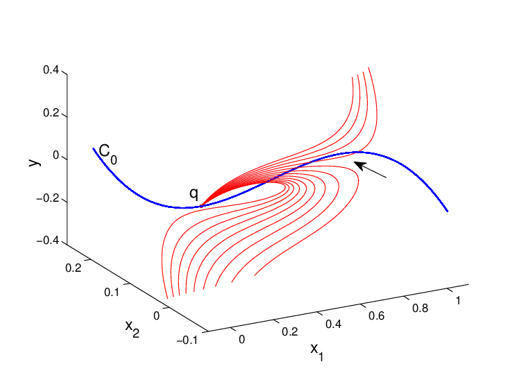
The geometry of the orbits along the upper branch of the C-curve is obtained by approximating it with two fast singular heteroclinic connections and parts of the slow manifolds and ; this process has been described several times in the literature when different methods were used to prove the existence of “fast waves” (see e.g. [29, 4, 32]).
4 Conclusions

Our results are summarized in the singular bifurcation diagram shown in Figure 12.
This figure shows information obtained by a combination of fast-slow decompositions, classical dynamical systems techniques and robust numerical algorithms that work for very small values of . It recovers and extends to smaller values of the CU-structure described in [5] for the FitzHugh-Nagumo equation. The U-shaped Hopf curve was computed with an explicit formula, and the homoclinic C-curve was determined by locating transitions between different dynamical behaviors separated by the homoclinic orbits. All the results shown as solid lines in Figure 12 have been obtained by considering a singular limit. The lines and as well as the slow flow bifurcation follow from the singular limit yielding the fast and slow subsystems of the FitzHugh-Nagumo equation (6). The analysis of canards and periodic orbits have been obtained from equations (17) and (18) where the singular limit was used (see Section 2.3). We have also shown the C- and U-curves in Figure 12 as dotted lines to orient the reader how the results from Proposition 5 and Conjecture 1 fit in.
We also observed that several dynamical phenomena are difficult to recover from the singular limit fast-slow decomposition. In particular, the codimension two generalized Hopf bifurcation does not seem to be observable from the singular limit analysis. Furthermore the homoclinic orbits can be constructed from the singular limits but it cannot be determined directly from the fast and slow subsystems that they are of Shilnikov-type.
The type of analysis pursued here seems to be very useful for other multiple time-scale problems involving multi-parameter bifurcation problems. In future work, we shall give a geometric analysis of the folding/turning mechanism of the homoclinic C-curve, a feature of this system we have not been able to determine directly from our singular limit analysis. That work relies upon new methods for calculating and which are invariant slow manifolds of “saddle-type” with both stable and unstable manifolds.
We end with brief historical remarks. The references cited in this paper discuss mathematical challenges posed by the FitzHugh-Nagumo equation, how these challenges have been analyzed and their relationship to general questions about multiple time-scale systems. Along the line in Figure 12 we encounter a perturbation problem regarding the persistence of homoclinic orbits that can be solved using Fenichel theory [45]. The point marks the connection between fast and slow waves in -parameter space which has been investigated in -parameter space in [38]. We view this codimension 2 connectivity as one of the key features of the FitzHugh-Nagumo system. The perturbation problem for homoclinic orbits close to the line was solved using several methods and was put into the context of multiple time-scale systems in [31, 32], where the Exchange Lemma overcame difficulties in tracking when it starts jumping away from . This theory provides rigorous foundations that support our numerical computations and their interpretation.
Acknowledgment: This research was partially supported by the National Science Foundation and Department of Energy.
References
- [1] D.G. Aronson and H.F. Weinberger. Nonlinear diffusion in population genetics, combustion, and nerve pulse propagation. in: Partial Differential Equations and Related Topics (Lecture Notes in Mathematics), 446:5–49, 1974.
- [2] K. Bold, C. Edwards, J. Guckenheimer, S. Guharay, K. Hoffman, Judith Hubbard, Ricardo Oliva, and Waren Weckesser. The forced van der pol equation 2: Canards in the reduced system. SIAM Journal of Applied Dynamical Systems, 2(4):570–608, 2003.
- [3] P. Brunovsky. Tracking invariant manifolds without differential forms. Acta Math. Univ. Comenianae, LXV(1):23–32, 1996.
- [4] Gail A. Carpenter. A geometric approach to singular perturbation problems with applications to nerve impulse equations. Journal of Differential Equations, 23:335–367, 1977.
- [5] A.R. Champneys, V. Kirk, E. Knobloch, B.E. Oldeman, and J. Sneyd. When shil’nikov meets hopf in excitable systems. SIAM Journal of Applied Dynamical Systems, 6(4), 2007.
- [6] Bo Deng. The existence of infinitely many traveling front and back waves in the fitzhugh-nagumo equations. SIAM J. Appl. Math., 22(6):1631–1650, 1991.
- [7] M. Diener. The canard unchained or how fast/slow dynamical systems bifurcate. The Mathematical Intelligencer, 6:38-48, 1984.
- [8] Francine Diener and Marc Diener. Nonstandard Analysis in Practice. Springer, 1995.
- [9] Freddy Dumortier. Techniques in the theory of local bifurcations: Blow-up, normal forms, nilpotent bifurcations, singular perturbations. in: Bifurcations and Periodic Orbits of Vector Fields [D. Schlomiuk (ed.)], pages 19–73, 1993.
- [10] Freddy Dumortier and R.Roussarie. Canard Cycles and Center Manifolds Memoirs of the American Mathematical Society, 121(577), 1996.
- [11] Wiktor Eckhaus. Relaxation oscillations including a standard chase on french ducks. Lecture Notes in Mathematics, 985:449–494, 1983.
- [12] V.I. Arnold (Ed.). Encyclopedia of Mathematical Sciences: Dynamical Systems V. Springer, 1994.
- [13] E.J. Doedel et al. Auto 97: Continuation and bifurcation software for ordinary differential equations. http://indy.cs.concordia.ca/auto, 1997.
- [14] E.J. Doedel et al. Auto 2000: Continuation and bifurcation software for ordinary differential equations (with homcont). http://cmvl.cs.concordia.ca/auto, 2000.
- [15] John W. Evans, Neil Fenichel, and John A. Feroe. Double impulse solutions in nerve axon equations. SIAM J. Appl. Math., 42(2):219–234, 1982.
- [16] Neil Fenichel. Persistence and smoothness of invariant manifolds for flows. Indiana University Mathematical Journal, 21:193–225, 1971.
- [17] Neil Fenichel. Asymptotic stability with rate conditions. Indiana University Mathematical Journal, 23:1109–1137, 1974.
- [18] Neil Fenichel. Asymptotic stability with rate conditions ii. Indiana University Mathematical Journal, 26:81–93, 1977.
- [19] Neil Fenichel. Geometric singular perturbation theory for ordinary differential equations. Journal of Differential Equations, 31:53–98, 1979.
- [20] R. FitzHugh. Mathematical models of threshold phenomena in the nerve membrane. Bull. Math. Biophysics, 17:257–269, 1955.
- [21] Gilberto Flores. Stability analysis for the slow traveling pulse of the fitzhugh-nagumo system. SIAM J. Math. Anal., 22(2):392–399, 1991.
- [22] W. Govaerts and Yu.A. Kuznetsov. Matcont. http://www.matcont.ugent.be/, 2008.
- [23] Johan Grasman. Asymptotic Methods for Relaxation Oscillations and Applications. Springer, 1987.
- [24] John Guckenheimer. Bifurcation and degenerate decomposition in multiple time scale dynamical systems. in: Nonlinear Dynamics and Chaos: Where do we go from here? Eds.: John Hogan, Alan Champneys and Bernd Krauskopf, pages 1–20, 2002.
- [25] John Guckenheimer. Global bifurcations of periodic orbits in the forced van der pol equation. in: Global Analysis of Dynamical Systems - Festschrift dedicated to Floris Takens. Eds.: Henk W. Broer, Bernd Krauskopf and Gert Vegter, pages 1–16, 2003.
- [26] John Guckenheimer. Bifurcations of relaxation oscillations. Normal forms, bifurcations and finiteness problems in differential equations, NATO Sci. Ser. II Math. Phys. Chem., 137:295–316, 2004.
- [27] John Guckenheimer, Kathleen Hoffman, and Warren Weckesser. The forced van der pol equation 1: The slow flow and its bifurcations. SIAM Journal of Applied Dynamical Systems, 2(1):1–35, 2003.
- [28] S.P. Hastings. Some mathematical problems from neurobiology. The American Mathematical Monthly, 82(9):881–895, 1975.
- [29] S.P. Hastings. On the existence of homoclinic and periodic orbits in the fitzhugh-nagumo equations. Quart. J. Math. Oxford, 2(27):123–134, 1976.
- [30] A.L. Hodgin and A.F. Huxley. A quantitative description of membrane current and its application to conduction and excitation in nerve. J. Physiol., 117:500–505, 1952.
- [31] C. Jones and N. Kopell. Tracking invariant manifolds with differential forms in singularly perturbed systems. Journal of Differential Equations, pages 64–88, 1994.
- [32] C. Jones, N. Kopell, and R. Langer. Construction of the fitzhugh-nagumo pulse using differential forms. in: Multiple-Time-Scale Dynamical Systems, pages 101–113, 2001.
- [33] Christopher K.R.T. Jones. Stability of the travelling wave solution of the fitzhugh-nagumo system. Transactions of the American Mathematical Society, 286(2):431–469, 1984.
- [34] Christopher K.R.T. Jones. Geometric Singular Perturbation Theory: in Dynamical Systems (Montecatini Terme, 1994). Springer, 1995.
- [35] Christopher K.R.T. Jones, Tasso J. Kaper, and Nancy Kopell. Tracking invariant manifolds up tp exponentially small errors. SIAM Journal of Mathematical Analysis, 27(2):558–577, 1996.
- [36] B. Krauskopf and T. Riess. A lin’s method approach to finding and continuing heteroclinic connections involving periodic orbits. Nonlinearity, 21(8):1655–1690, 2008.
- [37] M. Krupa and P. Szmolyan. Extending geometric singular perturbation theory to nonhyperbolic points - fold and canard points in two dimensions. SIAM J. Math. Anal., 33(2):286–314, 2001.
- [38] Martin Krupa, Bjoern Sandstede, and Peter Szmolyan. Fast and slow waves in the fitzhugh-nagumo equation. Journal of Differential Equations, 133:49–97, 1997.
- [39] Martin Krupa and Peter Szmolyan. Relaxation oscillation and canard explosion. Journal of Differential Equations, 174:312–368, 2001.
- [40] X-B Lin. Using melnikov’s method to solve shilnikov’s problems. Proc. Roy. Soc. Edinburgh, 116:295–325, 1990.
- [41] Alexandra Milik and Peter Szmolyan. Multiple time scales and canards in a chemical oscillator. in: Multiple-Time-Scale Dynamical Systems, Eds.: Christopher K.R.T. Jones (Editor) and Alexander I. Khibnik (Editor), 2001.
- [42] E.F. Mishchenko and N.Kh. Rozov. Differential Equations with Small Parameters and Relaxation Oscillations (translated from Russian). Plenum Press, 1980.
- [43] J. Nagumo, S. Arimoto, and S. Yoshizawa. An active pulse transmission line simulating nerve axon. Proc. IRE, 50:2061–2070, 1962.
- [44] C. Rocsoreanu, A. Georgescu, and N. Giurgiteanu. The FitzHugh-Nagumo Model - Bifurcation and Dynamics. Kluwer, 2000.
- [45] Peter Szmolyan. Transversal heteroclinic and homoclinic orbits in singular perturbation problems. Journal of Differential Equations, 92:252–281, 1991.
- [46] Peter Szmolyan and Martin Wechselberger. Canards in . Journal of Differential Equations, 177:419–453, 2001.