Gauss diagrams of real and virtual knots in the solid torus

Let $\mathcal{G}_{1}$ and $\mathcal{G}_{2}$ have the same underlying decorated Gauss diagram $G$. We call edges of a Gauss diagram the connected components of the complementary of its arrows. Up to elementary refinement moves of type I, we may assume that any edge of either $\mathcal{G}_{1}$ or $\mathcal{G}_{2}$ contains markings with all the same sign. Two such diagrams may then be assimilated to elements of the $\mathbb{Z}-$module freely generated by the edges of $G$, numbered from $e_{1}$ to $e_{2n}$, where $n$ denotes the number of arrows in $G$.

Notice that if $n\leq 1$, then $G$ only has one refinement up to type I moves. Now we assume $n\geq 2$.

Let $M\in\mathcal{M}_{n+1,2n}(\mathbb{Z})$ be a matrix whose arrows are defined as the distinguished loops of $G$, written in the basis $\left\{e_{i}\right\}$. We look at $M$ as a linear map $\mathbb{R}^{2n}\rightarrow\mathbb{R}^{n+1}$. With this description, the “difference” between $\mathcal{G}_{1}$ and $\mathcal{G}_{2}$ is nothing but an element of $\mathbb{Z}^{2n}\cap\text{Ker}M$ - a way of changing the integer assigned to each edge of $G$ without changing their sum on any distinguished loop. Since the distinguished loops of $G$ form a basis of $H_{1}(G)$, $M$ has maximal rank, i.e. $\text{dim}(\text{Ker}M)=n-1$. We are now going to prove that the refinement moves associated to any $n-1$ arrows of $G$ form a suitable basis of $\text{Ker}M$.

Let $A_{n}$ be any arrow of $G$. At least one of the $3$ or $4$ edges of $G$ that are adjacent to $A_{n}$ is also adjacent to another arrow $A_{n-1}$. Erase $A_{n-1}$: in the new Gauss diagram (if $n\geq 3$) there must be again an arrow $A_{n-2}$ with an adjacent edge in common with $A_{n}$. This means that in the original diagram $G$, it had an adjacent edge which was also adjacent to either $A_{n}$ or $A_{n-1}$, but certainly not any other arrow. Iterating this process, we get the arrows of $G$ into some order $\left(A_{i}\right)_{i=1}^{n}$ satisfying the following: if $x_{i}\in\text{Ker}M$ corresponds to the type II+ move associated to $A_{i}$, then

This implies not only that $\left\{x_{i}\right\}$ forms a basis of Ker$M$, but also that any element of $\mathbb{Z}^{2n}\cap\text{Ker}M$ has integer coordinates in that basis. So we may go from $\mathcal{G}_{1}$ to $\mathcal{G}_{2}$ by means of elementary moves of type I, II+ and II-. Finally, notice that the elementary move of type II- associated to some arrow is the sum of the type II+ moves associated to all the others. ∎

Fig.9 shows how to perform type I moves. Again a dashed arc represents a part of the knot with only virtual intersections. Both parts of the proof are fully based on the fundamental property of virtual crossings (Lemma 1.1).

To perform a type II move, we begin with two moves of type I (Fig.10, step 1). The two internal branches are chosen so close that they both (virtually) intersect the same other branches of the knot, which allows us to slide the real crossing, using virtual Reidemeister III move from Fig.3, all the way to the other side of $S$.

∎

Proposition 2.2 and Lemma 2.3 together imply that the common decorated Gauss diagram $G$ has a refinement $\mathcal{G}$ such that up to virtual Reidemeister moves, both knot diagrams write as the closure of a tangle with $T-$diagram $\mathcal{G}$. Now Proposition 1.9 concludes the proof. ∎

Recall that the valuations of a decorated Gauss diagram are the images of a basis of $H_{1}(G)$ into $H_{1}(\mathbb{R}\times\mathbb{S}^{1})$. If $D$ is not full then clearly every loop in its Gauss diagram has homology class $0$ in $\mathbb{R}\times\mathbb{S}^{1}$. Conversely, if $D$ is full, then its leftmost loop has homology class $1$. Since by assumption $D$ is real, this loop actually corresponds to a loop in $G$, because the two branches of any crossing are actually connected by an arrow. Since some loop has a nontrivial image, any basis must contain an element with a nontrivial image. ∎

If $D$ is isotopic to a knot diagram $D^{\prime}$ contained in a little disc, then put $\mathcal{G}^{\prime}=\mathcal{G}$ with all the markings removed, and choose a section $S$ that avoids $D^{\prime}$.

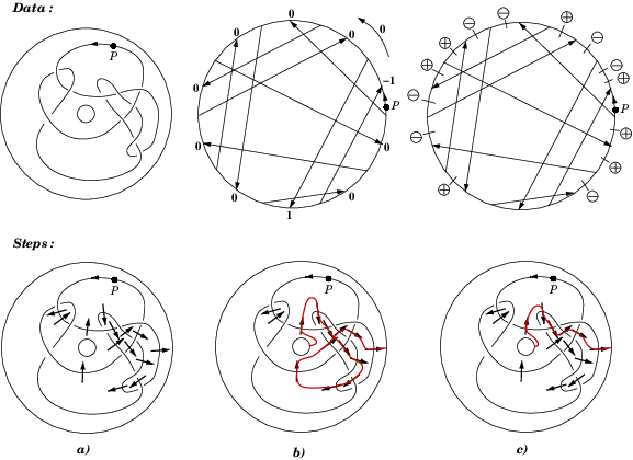
Now assume that $D$ is full. Draw the markings of $\mathcal{G}$ on $D$. Then replace each of them by a little arrow transverse to the knot diagram, that indicates the way a section should locally behave so as to give the marking (step a) on Fig.12). What we need to prove is that there is a path joining the two ends of $\mathbb{R}\times\mathbb{S}^{1}$, without self-intersection (so that some ambient isotopy can make it into a section $\mathbb{R}\times\left\{t\right\}$), and meeting $D$ only at the places and with directions indicated by the arrows ($\mathcal{G}^{\prime}$ being obtained by removing all the markings left away from that path).

We start to draw such a path $\gamma$ from the end corresponding to $-\infty$. Recall that the sum of the markings met by a loop in $\mathcal{G}$ is equal to its homology class in $\mathbb{R}\times\mathbb{S}^{1}$. Since the leftmost loop of $D$ has homology class $1$, there is at least one little arrow indicating a “way to leave” the component, and as soon as we have left it, there will be as many ways to come back as to leave again.

The internal loops have homology class $0$, so that each time $\gamma$ enters a component which is not the $+\infty$ end, the fact that it could come implies that there is necessarily a way to leave. So we are sure of eventually reaching $+\infty$ (step b) on Fig.12). Finally, if $\gamma$ ever crosses itself, just forget what happened between the two times it were at this point (step c) on Fig.12). ∎

Let $\mathcal{G}$ be a refinement of the common decorated Gauss diagram $G$, with minimal number of markings - notice that this number must be positive by Lemma 3.3. Then by Lemma 3.4 both knot diagrams write as the closure of a tangle with $T-$diagram $\mathcal{G}$. So all we need to prove is that there is only one way to draw a real tangle diagram representing $\mathcal{G}$ in the previous conditions.

First let us show that the connected components of such a tangle diagram are uniquely determined, so that the only possible choice left consists in their relative position in $\mathbb{R}\times\left[0,1\right]$.

We pick a marking in $\mathcal{G}$: it must correspond to the beginning of a strand. From there we follow the orientation of $\mathcal{G}$, collecting every piece of information we meet and using them to draw, step by step, a neighborhood of the strand (see Fig.13).

$\blacktriangleright$ When we encounter the endpoint of an arrow, its direction and sign completely determine the local picture (step a).

$\triangleright$ If we meet the second endpoint of some arrow, it means we have to join a piece of diagram already in the picture, and there is at most one way to do it: indeed, the ends of every strand must stay in the unbounded region of the plane, so that at the end we can glue them to the boundary of $\mathbb{R}\times\left[0,1\right]$ (step b). This point makes the crucial difference between Gauss diagram theories in $\mathbb{R}^{2}$ and $\mathbb{R}\times\mathbb{S}^{1}$.

$\triangleright$ When we finally meet a marking again, it is the end of the strand and we stop here (step c).

$\blacktriangleright$ If there are any, we pick an arrow which we have met at exactly one endpoint, and start over from the other one to extend the corresponding local incomplete picture (step d).

When this is all over, we have drawn what must be a connected component of any tangle representing $\mathcal{G}$, without making any choice (step e).

Each univalent vertex of these components has a type, $0$ or $1$, according to whether it is meant to be glued to either of the two sides of $\mathbb{R}\times\left[0,1\right]$. This side information is contained in $\mathcal{G}$, through the orientation and the sign of the markings. Let us call mates two univalent vertices that are meant to be identified when we finally close the tangle.

We claim that any of the components must contain both types of vertices. Otherwise, consider a tangle whose $T-$diagram is $\mathcal{G}$ (we know there is at least one), then $S^{\prime}$ on Fig.14 shows how to obtain a new refinement of $G$ with less markings than $\mathcal{G}$ - which is a contradiction.

So our components look like bowels, as pictured in Fig.14, and it remains to show that we can read on $\mathcal{G}$ in what order they shall be.

First, the leftmost of them is uniquely determined by the property that its left “boundary path” joins two mates (it is meant to become the leftmost loop of the knot). Indeed, if there were two or more components with this property, the tangle would close into a disconnected diagram, and certainly not into a knot.

Now assume that we have been able to determine which are the $k$ leftmost components in a unique way. Look at the bottom ends of the picture they form.

$\triangleright$ Take the leftmost of them whose mate is not already in the picture: the component containing its mate is necessarily the next we should draw.

$\triangleright$ If all bottom ends already have their mate, look at the upper ends and repeat the same procedure.

$\triangleright$ If all upper ends also have their mate, then it means that the two rightmost ends in the picture are mates, and belong to one and the same component: this characterizes the rightmost loop of the knot, so the picture is actually complete.

∎

The “if” part is trivial. Propositions 4.8 and 4.9 together prove the converse for positive $T-$diagrams, and Corollary 4.6 shows that this is enough. ∎

For the sake of simplicity, we will write $V_{0}$, $W_{0}$, etc., instead of $V_{v_{0}}$, $W_{v_{0}}$, etc., and $\varepsilon(k)$ will stand for the sign of $k$. Fix $i$ such that $e_{i}\notin V$, and set $W=V\oplus\mathbb{Z}e_{i}$. The proof is in two steps. First, we show that $W$ still has property $\mathfrak{P}$; then that $\phi$ extends to $\psi:W\rightarrow\mathbb{Z}$ such that $\psi(W_{0})\subset\mathbb{N}$. The lemma follows by iteration of these two steps.

Let $w=v+k.e_{i}\in W$ with $v\in V$ and $k\in\mathbb{Z}$. Write $v$ as a sum of units $v_{l}$ lying in $V_{v}$. Note that $\varepsilon_{j}(w)=\varepsilon_{j}(v)$ for $j\neq i$.

Case 1: $\varepsilon_{i}(v)\in\left\{0,\varepsilon(k)\right\}$. Then the $v_{l}$’s also lie in $W_{w}$, and so does the unit $\varepsilon(k).e_{i}$, so we are happy with:

.

Case 2: $\varepsilon_{i}(v)=-\varepsilon(k)$. Put $L:=\left\{l\mid\varepsilon_{i}(v_{l})\neq 0\right\}$. Notice that:

$\triangleright$ If $\lvert k\rvert<\sharp L$, then $\varepsilon_{i}(w)=\varepsilon_{i}(v)$, which implies that $\varepsilon(v_{l})\leq\varepsilon(w)$ and $v_{l}$ is a unit of $W_{w}$ even for $l\in L$, and if we pick any $k$ elements of $L$, say $l_{1},\ldots,l_{k}$, then:

$\triangleright$ If $\lvert k\rvert=\sharp L$, then simply:

$\triangleright$ If $\lvert k\rvert>\sharp L$, then $\varepsilon_{i}(w)=\varepsilon(k)$, which means $\varepsilon(k).e_{i}$ is a unit of $W_{w}$, and:

In any case we have a positive decomposition of $w$ along units of $W_{w}$. So we have proved that $W$ still has property $\mathfrak{P}$.

We now want to set $\psi_{\mid V}=\phi$ and give a value to $\psi(e_{i})$ so that $\psi\left(W_{0}\right)\subset\mathbb{N}$. First, notice that since by assumption $v_{0}$ has no zero coordinate, either of $e_{i}$ and $-e_{i}$ lies in $W_{0}$, namely $\varepsilon_{i}(v_{0}).e_{i}$, so we need to ensure that $\psi(\varepsilon_{i}(v_{0}).e_{i})\geq 0$. Besides this, every element $w=v+k.e_{i}\in W_{0}$ with $k\neq 0$ gives a condition, namely $\psi(e_{i})\geq-\frac{1}{k}\psi(v)$ if $k>0$, $\psi(e_{i})\leq-\frac{1}{k}\psi(v)$ if $k<0$. Let us look first at the conditions yielded by $k=\pm 1$. If we set:

then all the $k=\pm 1$-conditions reduce to:

The assumption that $v_{0}$ has no zero coordinate ensures that $\left\{v_{0}\pm e_{i}\right\}\subset W_{0}$, so that $\mathcal{K}_{-1}\text{ and }\mathcal{K}_{+1}$ are not empty, i.e. $\,-\infty<\textsl{sup}\,\mathcal{K}_{+1}$ and $\textsl{inf}\,\mathcal{K}_{-1}<+\infty$.

Assume now that $\varepsilon_{i}(v_{0})=+1$, and set $\psi(e_{i})=\textsl{inf}\,\mathcal{K}_{-1}$. Were it $-1$, we would set instead $\psi(e_{i})=\textsl{sup}\,\mathcal{K}_{+1}$ and everything would work exactly the same way. Since $\varepsilon_{i}(v_{0})>0$:

This shows that $\psi(e_{i})=\textsl{inf}\,\mathcal{K}_{-1}$ is non-negative: the condition $\psi(\varepsilon_{i}(v_{0}).e_{i})\geq 0$ is filled.

Let $w_{1}=v_{1}+e_{i}$ and $w_{2}=v_{2}-e_{i}$ lie in $W_{0}$. Then:

So we have proved that:

and $\psi(e_{i})$ is an integer with the required sign, satisfying all $k=\pm 1$-conditions.

Now we claim that these elementary conditions are enough for all the others to hold. Indeed, let $k$ be any integer and $v\in V$ such that $w=v+k.e_{i}\in W_{0}$. Throughout the proof that $W$ satisfies the property $\mathfrak{P}$, we actually showed that such a $w$ is a sum of units of $W_{w}$ of either of the forms $v_{l}+e_{i}$, $v_{l}-e_{i}$, $v_{l}$, $\varepsilon_{i}(v_{0}).e_{i}$, where the $v_{l}$’s stand for units of $V_{v}$. Since $w\in W_{0}\Rightarrow W_{w}\subset W_{0}$, such units have non-negative image by $\psi$, and therefrom so does $w$. ∎

The “only if” part is trivial. Let $G$ be a weakly admissible diagram, with $n$ arrows. Recall that the edges of $G$ are the connected components of the complementary of its arrows. We embed $H_{1}(G)$ into $\mathbb{Z}^{2n}=\bigoplus\mathbb{Z}e_{i}$ in the following way: number the edges of $G$ from $1$ to $2n$, then send every distinguished loop in $G$ to the sum of the $e_{i}$’s corresponding to the edges it goes through, and send the fundamental class of the circle to the sum of all $e_{i}$’s. Call this embedding $\iota$, and set $V:=\iota(H_{1}(G))$. Since $\iota$ defines an isomorphism between $V$ and $H_{1}(G)$, we may set:

Now all we need to do is extend the map $\phi$ into an element of $\bigoplus\mathbb{N}e_{i}^{*}$: the coefficient against $e_{i}^{*}$ will indicate how many markings we shall put on the $i$-th edge of $G$.

First, we see that $V$ satisfies the property $\mathfrak{P}$: indeed, this is a general fact about $1-$dimensional cellular spaces. Shrink every arrow of $G$ to a point (vertex), so that the $e_{i}$’s fully describe its cellular structure. Then let $v\in V$ write as $\iota\left(x=\sum x_{i}e_{i}\right)$. Let $\gamma$ be a path in $G$ corresponding as a $1-$chain to $\varepsilon_{i_{1}}(x)e_{i_{1}}$, where $i_{1}$ is such that $x_{i_{1}}\neq 0$. If the two ends of $e_{i_{1}}$ were joined by an arrow, then $\gamma$ is a loop and we stop here. Otherwise, since $x$ is a cycle, there must be some $i_{2}$ such that $\varepsilon_{i_{2}}(x)e_{i_{2}}$ is a path that starts where $\gamma$ ends. So we put $\gamma=\varepsilon_{i_{1}}(x)e_{i_{1}}+\varepsilon_{i_{2}}(x)e_{i_{2}}$, and iterate this process until $\gamma$ meets some vertex $A$ for the second time. Then we forget what happened before $\gamma$ first met $A$. What remains is a loop, whose image by $\iota$ is a unit of $V_{v}$. Repeating this with $v-\iota(\gamma)$, and so on, we split $v$ as a sum of units of $V_{v}$.

By the same process, we see that an element of $V\cap\mathbb{N}^{2n}$ corresponds through $\iota$ to the sum of the fundamental classes of loops in $G$ that can be chosen so as to respect orientation. So if we set $v_{0}=\sum e_{i}\in V$, then the weak admissibility of $G$ implies that $\phi$ takes $V_{0}=V\cap\mathbb{N}^{2n}$ into $\mathbb{N}$. Since $v_{0}$ has no zero coordinate, lemma 4.3 applies and gives the required extension. ∎

Note that if there is no arrow, then the diagram is admissible and the lemma is true. We assume from now on that $D$ has at least one arrow.

For positive diagrams, being admissible is equivalent to satisfying the property that every nontrivial and orientation respecting loop meets at least one marking. So assume that each arrow has a level, but that some loop fails to meet any marking. There must be at least one arrow involved in that loop. If not, then it would go all the way around the whole circle, and meet markings since the diagram is positive: that is a contradiction. Remove the arrows which are not involved in the loop. Those remaining had a well defined level, so they still have one in the new diagram, and so at least one of them, say $A$, has level $1$ in the new diagram. It means that each endpoint of $A$ is directly preceded by a marking. Since our loop goes along $A$, and respects the orientation of the circle, it must meet one of them: that is a contradiction.

Conversely, assume that some arrow has no level, and remove all of those which have one. In this new diagram, pick a marking which is not directly followed by another, i.e. which is directly followed by the endpoint of an arrow. We start our loop at this endpoint. Go along the arrow. The other endpoint cannot be also preceded by a marking, or the arrow would have a level. So go back along the circle until we find the endpoint of an arrow that is directly preceded by a marking. Then iterate those two steps: we must loop, since there is a finite number of arrows, and the loop we created avoids every marking. ∎

Every real crossing of a virtual braid which may be isotoped into the lowest corresponds to an arrow of level $1$ in the associated $T-$diagram. Removing these arrows amounts to replacing the real crossings by virtual ones. Until there is no more real crossing, there will always be a lowest one. This proves the “only if” part.

Assume that each arrow of a positive diagram has a level. Let $k$ be the global marking of the circle, and let $l$ be the maximal level of the arrows. Cut the circle at every marking, so as to obtain a diagram based on a union of $k$ segments, and embed it into $\mathbb{R}\times\left[0,l+1\right]$, in such a way that the segments are oriented from bottom to top, and such that each arrow of level $i$ is contained in $\mathbb{R}\times\left\{i\right\}$. The fact that each arrow has a level is equivalent to the existence of such an embedding. Now at each level make the strands cross each other as indicated by the arrows, by a homotopy that keeps the $i+1/2$-levels untouched. Declare virtual every additional crossing needed to do that. Finally, add to the top a totally virtual braid corresponding to the permutation defined by the way the strands were originally glued together in the circle, so that the resulting braid closes into a knot with the required $T-$diagram. ∎

References

- [F1] T. Fiedler, Gauss diagram invariants for knots and links, Mathematics and its Applications, Vol. 552, Kluwer Academic Publishers, 2001.
- [F2] T. Fiedler, Gauss diagram invariants for knots which are not closed braids, Math. Proc. Camb. Phil. Soc. 135(2003), 335-348.
- [Gor] V. Goryunov, Finite Order Invariants of Framed Knots in a solid torus and in Arnold’s -Theory of plane curves, “Geometry and Physics”, Lecture Notes in Pure Appl. Math. 184, M. Dekker, New York, 1996, 549-556.
- [G-P-V] M. Goussarov, M. Polyak and O. Viro, Finite-type invariants of classical and virtual knots,. Topology 39 (2000), no. 5, 10451068.
- [Kal] E. Kalfagianni, Finite type invariants for knots in three manifolds, Topology 37-3 (1998) 673-707.
- [K1] L. H. Kauffman, Talks at: the MSRI Meeting in January 1997; AMS Meeting at the University of Maryland, College Park in March 1997; Isaac Newton Institute Lecture in November 1997; Knots in Hellas Meeting in Delphi, Greece in July 1998; APCTP-NANKAI Symposium on Yang-Baxter Systems, Non-Linear Models and Applications at Seoul, Korea in October 1998.
- [K2] L. H. Kauffman, Virtual knot theory, European Journal of Combinatorics 20 (1999) 663-690.
- [P-V] M. Polyak and O. Viro, Gauss diagram formulas for Vassiliev invariants, Int. Math. Res. Notices 11 (1994) 445-453.
Institut de Mathematiques de Toulouse
Universite Paul Sabatier et CNRS (UMR 5219)
118, route de Narbonne
31062 Toulouse Cedex 09, France
mortier@math.ups-tlse.fr