Bethe Ansatz approach to the pairing fluctuations in the mesoscopic regime
Abstract
We review the exact treatment of the pairing correlation functions in the canonical ensemble. The key for the calculations has been provided by relating the discrete BCS model to known integrable theories corresponding to the so called Gaudin magnets with suitable boundary terms. In the present case the correlation functions can be accessed beyond the formal level, allowing the description of the cross-over from few electrons to the thermodynamic limit. In particular, we summarize the results on the finite size scaling behavior of the canonical pairing clarifying some puzzles emerged in the past. Some recent developments and applications are outlined.
PACS: 02.30.Ik , 74.20.Fg , 03.65.Fd
I Introduction
When a small attractive interaction is switched on in a Fermi gas, bound states are formed non-perturbatively[1]. This is the essence of the BCS pairing phenomenon [2, 3, 4, 5], leading ultimately to a phase transition as a result of a competition between the kinetic energy and the tendency of Cooper pairs to condense [1, 2]. The transition is usually described as a gauge symmetry breaking where the phase of the order parameter acquires a fixed value. Nevertheless it should be observed that because phase and number are conjugate variables, a definite value of the phase can be consistently reached only in open systems, where the number of Cooper pairs can fluctuate. The thermodynamics of macroscopic systems, however, is not affected by equilibrium fluctuations (grand-canonical and canonical statistical mechanics are equivalent in the thermodynamic limit). Accordingly, for macroscopic systems the BCS condensate is a quantum coherent state of Cooper pairs characterized by a well defined order parameter, which is the Cooper-pair binding energy [1, 6]. Away from the thermodynamic limit, it becomes delicate when speaking of the existence of the BCS state if the BCS pairing energy overlaps only a few energy electronic levels (the electrons level spacing is inversely proportional to the volume of the system). The point was famously remarked by Anderson with the question: “What is the size limit for a metallic particle to have superconducting properties?” [7]. This conceptual challenge has been revived significantly by experiments on isolated metallic grains of nanoscopic size [8]. The crucial aspect in the experiments is that the number of electrons inside the grain is fixed due to the typically very low capacitance of the sample. Therefore the standard superconducting order parameter exactly vanishes (the mean field approximation in the grand canonical ensemble is inappropriate). For BCS theory, the quantity playing the role of the “order parameter” is the pairing correlation function where are quantum numbers labeling electronic energy levels.
Canonical pairing fluctuations were first analyzed numerically [9] in order to study the physics of metallic nano-grains[10]. In such mesoscopic regimes the pairing phenomenon appears as a cross-over region dominated by superconducting fluctuations sized by the ratio [9]. Because the gauge symmetry cannot be broken at finite sizes, the system is characterized by these correlations (instead of a local observable). Interestingly, such a physical regime is shared with other important physical situations, notably in nuclei [11], and more recently in systems of confined degenerate alkali Fermi gases [12, 13]. Here, we comment that for at quantum degeneracy, the mesoscopic regime can be achieved with (corresponding to a confinement frequency of ) [12, 14] . In turn, because the BCS order parameter is coherent on the length scale , mesoscopic fluctuations in the atomic gas are important for small enough cloud size [15].
Since the system in mesoscopic cross-over regimes is characterized by strong quantum fluctuations, its physical behavior is very sensitive to the approximations employed and therefore exact results play an important role. The BCS model was solved exactly in 1964 with the seminal contributions by Richardson and Sherman [16]. The strategy they adopted is in the spirit very close to the coordinate Bethe ansatz: first they considered the Cooper pairs as effective bosonic particles; then they were able to incorporate the constraint coming from the actual fermionic statistics into the many-body wave function. In 1967 Gaudin [17] realized that the Richardson solution can be obtained with a variation of an approach he had pursued to solve the so-called Gaudin magnet [18]. The Richardson solution remained unnoticed by the condensed matter community until the late ninety’s, when it was re-discovered rendering an understanding of the low temperature physics of metallic grains [10] and later on for various applications in nuclear physics [19] and cold atoms [20].
Even with the knowledge of the exact solution for the spectrum of the system, the computation of the correlation function is a highly non-trivial task. In essence, the complications arise because in the correlation functions the eigenstates of the Hamiltonian are not easily expressed in terms of the ’natural’ states the operator acts on. Therefore an exceedingly complicated combinatorial problem arises involving (sums of) scalar products between Bethe eingenstates [21]. Using the exact eigenstates of the Hamiltonian, the diagonal pairing correlation function was obtained by Richardson although it was not evaluated explicitly [22]. A key progress for accessing the correlation functions exactly came from the observation that the BCS model belongs to the class of models that can be studied by the powerful techniques developed within the Quantum Inverse Scattering Method (QISM) [21]. Specifically, the BCS model is indeed a twisted Gaudin magnet [23, 24, 25, 26] related to disordered six vertex models [27, 24]. The first assault on the problem with QISM protocols was done in Ref.[28] where various correlation functions have been computed. A major simplification of the formulas was achieved by Zhou et al. [26] by application of the so called Slavnov formula for the calculation of the scalar products between Bethe states [29] together with the ’solution of the inverse problem’ [30, 31]. Correlation functions have been expressed as the sum of certain determinants. The ultimate progress has been achieved by Faribault, Calabrese and Caux who further reduced the complexity involved in the calculations, by applying certain reduction formulas for the determinants[32].
The aim of this article is to review the path we summarized above. In Section II we intoduce the BCS model and highlight its integrability. In Section III, we comment on the derivation of correlation functions by means of generating functions. Section IV is devoted to determinant representations of correlation functions making use of the solution to the inverse problem together with the reduction formulas worked out in [32] . Section V is focused on the pairing amplitute in the canonical ensemble. Section VI has a short view on the thermodynamic limit of the model. Section VII presents further ramifications.
II The BCS model
The BCS Hamiltonian is
| (1) |
is the pairing coupling constant; the quantum numbers label the single particle energy levels which are doubly degenerate since labels electron spin states; and are annihilation and number operators, respectively.
In the following we explain the connection of the BCS model with the -Gaudin model. For this goal we introduce the fundamental realization of in terms of electron pairs . The “lowest” weight module is generated by the vacuum vector , , where is the “lowest” weight ( for spin , which is the case of interest here [35]). The quadratic Casimir operator is , . The bilinear combinations and can be expressed in terms of Casimir and Cartan operators
| (2) |
The key observation is that the constants of the motion of the model Hamiltonian (1) can be obtained by the QISM. The method follows an ’inverse’ procedure to obtain a Hamiltonian that is integrable by construction. The starting point is to find a couple of matrices, and satisfying the Yang-Baxter equation
| (3) |
where is the spectral parameter. For the present case, the relevant matrices can be obtained through
| (4) |
where is the vector of Pauli matrices, and depending on the arbitrary parameter . The –matrix corresponds to and in (4) while the Lax matrix is obtained as
| (5) |
defines the column-to-column and row-to-row scattering matrices, respectively, of the two dimensional six vertex model with inhomogeneities [21]. The monodromy matrix
| (6) |
satisfies the Yang-Baxter equation
| (7) |
The twisted monodromy matrix
| (8) |
is then
| (9) |
It satisfies the Yang-Baxter equation as well due to . The transfer matrix is the trace (over the auxiliary space) of the monodromy matrix
| (10) |
The latter is a generating function of integrals of the motion of the theory because they commute at different values of spectral parameters: . The expansion generates a hierarchy of integrable systems since
| (11) |
The sum is on ordered partitions of including .
The first non trivial terms of the transfer matrix are
| (12) |
where
| (13) |
and are spin vectors; ). The operators (13) define the twisted Gaudin magnet, where holds. By these integrals of the motion, the BCS model becomes connected with the Gaudin Hamiltonians as the Hamiltonian (1) can be expressed in terms of as
| (14) |
which is manifestly integrable [23]:
| (15) |
The exact eigenstates of the BCS model [16, 18] are obtained first by diagonalizing :
| (16) |
where the Bethe vectors are
| (17) |
Then the eigenstates of [27] are obtained by the quasiclassical expansion of the Eq. (16) with . results to be
| (18) |
where
| (19) | |||||
| (20) |
and the rapidities with given by the Richardson equations
| (21) |
Finally the eigenvalues of are obtained via (14): with . Throughout the article we will consider the half filling case , unless it is stated differently.
We observe that the operators (19) span the infinite dimensional Gaudin algebra . The lowest weight module of is generated by the vacuum : wheren is the lowest weight of . We observe that the integrability of the BCS model can be obtained as an algebraic property of . In fact the mutual commutativity of descends from the relation between ( are residues of in ) and invariants (trace and quantum determinant[27]) of :
| (22) |
where is a twisted Casimir operator
| (23) | |||||
and
| (24) |
The property is the origin of the integrability of the BCS model. Therefore finding the spectrum of the BCS model means finding the representations of a twisted Gaudin algebra (labeled by its Casimir operator).
We mention that the Richardson equations (21) are intimately related to the algebraic structure of in that they act as constraints on the lowest weight . Thus, the difference between the BCS and Gaudin model amounts to a different constraint imposed on the lowest weight vector of which leads to different sets , ( is spanned by the solutions of (21) when ). We will use this fact to extend the Sklyanin theorem [34] to the BCS model.
In the next sections we will be focusing on the following -point charge and pairing correlation functions (CF)
| (25) |
| (26) |
The vectors
are exact -pair eigenstates of (1) (see Eqs. (18), (19)). Here, we observe that the evaluation of the CF’s (like (25), (26)) proceeds along the action of local operators, say , onto the Bethe states, the latter involving a collective reorganization of the vectors of the local Hilbert space . Therefore, for any fixed Bethe root , has to be commuted with to finally act on the vacuum . This gives rise to a problem of combinatorial nature, whose solution is a non trivial task. In the next section we will look explicitely tame the combinatorics for the special case of (25), (26).
III Generating function for CF
In [34] Sklyanin suggested how the combinatoric complications involved in the calculation of the correlation functions can be overcome resorting the Generating Function (GF) technique. He applied it [27] to the Gaudin model [18]. The key role in his approach is played by a reordering making use of the Baker–Campbell–Hausdorff (BCH) formula for elements of the loop group associated with the Gaudin algebra . In this section we exploit the common algebraic root of the Gaudin and BCS models to extend the Sklyanin theorem to the BCS model. The GF we will be looking at, is
| (27) |
where the sets are (in general distinct) sets of solutions of the Richardson equations (21); ; . The order of the correlation is the cardinality of : ; and are fixed by the number of pairs . For instance, the one and two point CFs correspond to and respectively.
Now we present the Sklyanin theorem for the GF of the
Gaudin model and apply it to the BCS model.
Therefore we need the notation of
the set of coordinated partitions
of the sets
(see Ref. [34]):
the partition is a set of triplets
; the triplet is
, where
,
and
such that .
The GF has been evaluated for the Gaudin
model exploiting the BCH formula
for
the loop group generated by
where and are meromorphic functions for with residues respectively [34]. This formula allows to rearrange the products between loop group elements in (27)
Sklyanin proved the following theorem [35].
Theorem. is given by the formula
| (28) | |||||
where
and .
is a polynomial
in with integer coefficients.
Expression (28) depends only on the sets
and [34, 37];
for the Gaudin model is a set of
solutions of (21) for ;
for the BCS model is a set of solutions of the
Richardson equations (21) for generic .
The scalar products of Bethe states (and their norms)
are a corollary of the Sklyanin theorem (28)
for :
.
Its consent with the determinant
formulas[18, 22] has been elucidated in
Refs.[34, 37].
We point out that the GF (27)
has simple poles in the set . This will play
a key role in the following.
Correlation functions. The charge and pairing CFs are matrix elements of the Lie algebra (instead of elements of ) using vector states of . The projection from the loop algebra on its Lie algebra is performed by taking the residue of in the poles for , . The charge CFs (25) are
| (29) |
where involve and means . Using (28) yields
| (30) | |||
where ; . The quantity is
| (31) | |||
where and are elements appearing singly and doubly in respectively. The pairing CF (26) can be extracted from where the vectors in (27) are and . Then is
| (32) |
is then calculated using the Sklyanin theorem. For formula (32) gives
| (33) | |||
where and is one of and ;
The pairing CF for can be obtained by a variation of the procedure depicted above:
But in the present case () it is more convenient employing the formula (30) because .
We comment that practical use of the formulas is limited by the vastly increasing number of partitions, which depends on the number of pairs and the order of the CF . We want to emphasize that no complete knowledge of all the eigenstates is required. It doesn’t show any dependence of the Hilbert space dimension either. We finally point out that the results apply to arbitrary (i.e. any degeneracy of the single particle levels).
IV Determinant representation of the Correlation Functions
In this section we will sketch how the formula obtained above can be simplified by recasting the CF’s into sums of determinants of certain matrices. As it was remarked above the scalar products between the BCS Bethe states can be expressed as determinants. Within the formalism we exploited in the previous section (see Eq.(28)) in fact
| (34) |
where can be written as
| (35) |
Sklyanin proved[27] that can be indeed written as a polynomial that is linear in each of , (see Eq. 21). Consistently with Richardson’s old result [22], it can be expressed as a sum of determinants
| (36) |
where is an element of the symmetric group and is defined as
A major simplification was achieved by Slavnov who was able to express the scalar product as a single determinant [29]. Therefore the Eq.(36) can be recast into
| (37) | |||||
As discussed in Sect.II the CF’s of the BCS model are identical to those of the Gaudin model, with the parameters satisfying Richardson’s equations (21) instead of the Gaudin-equations. The entries of the matrix are
| (38) | |||||
The norms of the states are obtained for in (37) and give where is the Gaudin matrix given by
| (39) |
The various stages of the calculation of CF’s proceed through certain recurrence formulas involving (37) as a basic ingredient (see [21] for the details). Therefore the CF’s result to be determinants as well. We comment that such a simplification was first achieved after a tour de force on integrable spin theories (beyond the quasi-classical expansion) leading to the so called solution of the inverse problem [30, 31]. The main accomplishment is that the lattice spin variables are expressed in terms of the entries of the monodromy matrix , , , in a closed (and simple) form. This allows to evaluate the CF’s in the non-local Hilbert space spanned by the Bethe vectors (instead of expressing the Bethe states in ). Zhou et al. [26] calculated the relevant quantities for the BCS model through the quasi-classical limit (12), generalizing the solution of the inverse problem to non-fundamental integrable spin theories (where the auxiliary and the quantum spaces have different dimensions). The formulae read [26]
with being essentially the total , and being the transfer matrix. The form factors are obtained as [30]
| (40) | |||
| (41) |
where and indicate Bethe states with and rapidities respectively. The matrix elements of and given by
is the matrix obtained from by deleting the last row and column and replacing by in the matrix elements. Here, we assume that both and are solutions to Richardson’s Bethe equations (21).
The two-point correlation functions are
| (42) |
Here, the hat denotes that the corresponding parameter is not present in the set. Since is a solution of the Bethe equations, is the form factor given before, while
| (43) |
with
In (43) is assumed, and it is zero if .
The expression for the charge CF can be obtained from the form factors and CF above[32]:
| (44) | |||
The static CF of interest here are obtained with .
IV.1 Reduction formulas
The last significant progress for the evaluation of the CF for was pursued by Faribault, Calabrese and Caux[32]. They managed to reduce the complexity of the above expressions to sums over only determinants.
Both and involve the evaluation of the form factors (40) and (43) for . In such a limit the CF are still a sum of two terms, each one involving sums of determinants of modified Gaudin matrices. In Ref. [32] the specific symmetry of the Richardson equations was exploited to reduce the CF to a single term expressed as a sum of determinants (see [32] for the detailed calculations). In this way, the final result for the correlation function is
| (45) |
where
| (46) |
Here,
| (47) | |||||
| (48) |
Similarly is given by [32]
| (49) |
The formulas obtained above for the correlation functions are completely general and are valid for any choice of the Hamiltonian parameters and (with some caveat in the limit of coinciding energies). The low level of complexity of this representation as sum of determinants of by matrices allows one to have access to the static correlation functions for systems with a reasonable number of pairs.
V Canonical pairing fluctuations
In the canonical ensemble the conventional BCS order parameter is vanishing exactly. Nevertheless the pairing instability can be characterized by studying the correlation function
| (50) |
indicating the tendency that electrons form Cooper pairs instead of uncorrelated electrons. The canonical BCS order parameter is[39, 9]
| (51) |
which in the limit of large volume and large reduces to the BCS value (see Sect.VI). We observe that, in contrast with a normal Fermi gas, a system with pairing instability will take an energetic advantage by increasing for fixed (because the phase space available for coherence is enlarged). Therefore, energy correlations are short ranged in a normal Fermi gas and long ranged in the presence of a pairing coherence. Accordingly, the footprint for an ongoing pairing instability is a finite size scaling ansatz
| (52) |


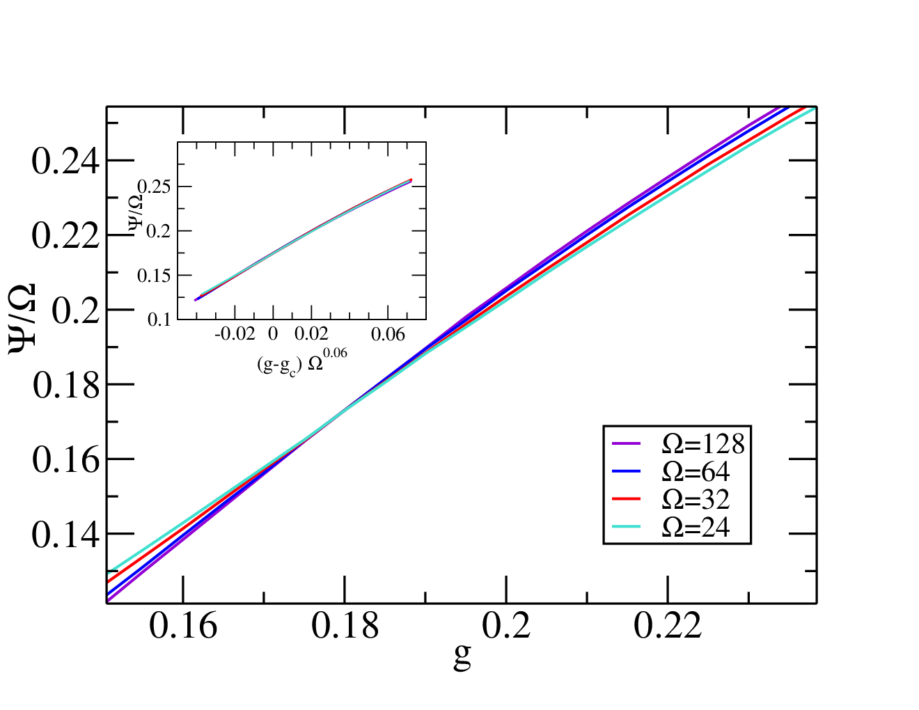
The above quantity was evaluated exploiting the exact formulas (30) and (41). The rapidities involved in the equations at finite size are obtained by solving the Richardson equations numerically for the model parameters, which here are equally spaced single particle energy levels and half filling (see Ref.[40] for the details). The results for are shown in Figs. 1 and 2. Whereas the former shows the dependence at fixed , in the latter each plot consists of the various curves at fixed (=0.1, 0.2, 0.4, 0.7) for varying . It is clear that the results tend to the BCS result. In Ref.[32] was noticed that this convergence is the slower, the smaller is: for the maximum at is only 90% close to the asymptotic result wheras at the result is already at 99.8%. In Fig. 3 the order parameter as a function of for several values of is shown and compared with the BCS result: for , is almost indistinguishable from its limiting value for large enough .


The scaling of was originally obtained in [9] for small size at a given value of the pairing coupling (see the caption of Fig.4). In Ref.[28] a further scaling point was evidenced (see the caption of Fig.5). In order to extract the finite-size scaling, was taken in consideration for different valus for and . At a scaling point all these curves cross () as shown in Fig. 5. The physical meaning of two apparent “scaling points” was unclear and deserved further analysis. This analyis was significantly extended in [32], but without any scaling analysis. However, there is no second scaling point visible in their analysis for larger pair number (). In figure 6 we present the data collapse of the data of Ref. [32]. The value for is in accordance with with an error about . The second coefficient leads to the searched-for data collapse.
It is instructive that the computed leading term of for large and
| (53) |
coincides with that of Ref. 36. Instead, for small and large
| (54) |
The independent result for large and the dependence at small gives a hint towards the non-perturbative nature of superconductivity. Further studies on the finite size corrections of the BCS pairing amplitude were performed in[41].
We close the discussion on the canonical pairing fluctuations
mentioning the relation between and the
Onsager-Penrose-Yang parameter [42] for the long-range
off-diagonal order,
taking into account the effect of non-diagonal correlations.
Although
can be obtained with the formulas for ,
a much easier route is to apply the Hellmann-Feynman theorem:
| (55) |
where is the ground state energy of the BCS model. In the thermodynamic limit . However, the two quantities are independent for finite sizes. Tian et al. [43] proved that and satisfy the following relations for any value of and
| (56) |
For these are trivial bounds, but not so for finite .
VI Thermodynamic limit
The Richardson equations (21) admit an electrostatic analogy [16, 18, 44, 45], where the eigenenergies
and solutions
both are interpreted as point charges
of the strengths and respectively. The thermodynamic limit is
performed making use of this analogy.
Define
| (57) | |||||
| (58) | |||||
| (59) |
This choice leaves the Debeye-shell invariant. Inserting this into the Richardson equation (21), cancels and we obtain
| (60) |

Following the works [16, 18] the BCS-gap is the imaginary opening of the arc solving the Richardson equations, (see Fig. 7), and the gap equation becomes
| (61) | |||||
| (62) |
where () is the multiplicity of the level . This resuls in the known expression for the equally spaced model. A good summary of Gaudin’s article together with a modern numerical analysis of the solutions for the BCS-model is found in [44]. The generalization of the electrostatic analogy to more general settings (the trigonometric and hyperbolic BCS-model) can be seen in [45].
VII Further directions
In this article we have reviewed the current understandings of the mesoscopic fluctuations of the pairing instability based on Bethe ansatz techniques. The relevant quantity is a correlation function (CF), where the physical observables are evaluated as a static expectation value in the eigenstates of the Hamiltonian. The progress in the field of exact solutions are mature enough to allow an exhaustive analyis of superconductivity from mesoscopic regimes to thermodynamic limit at equilibrium. An important piece of information, however, comes from the study of the system out of equilibrium. The typical picture is provided by transport experiments were the dynamical CF, , are the interesting quantities to be calculated. The formula for involve an additional level of complexity. The basic ingredients are off diagonal correlations, namely static CF between different eigenstates. The first exact off-diagonal CF for the BCS-model obtained in [28] could only be calculated for very small sizes. The better performance of the determinant expression in [26] could be even further improved in [32] to make reasonably higher pair numbers accessible. Nevertheless, this is not the end of the story because in principle all the off-diagonal CFs are involved in . Fortunately, the problem can be simplified for the BCS model because the eigenstates do not contain the coupling constant explicitly. In a very relevant paper, Faribault, Calabrese and Caux combined numerical and analytical analysis to realize that indeed only a relatively small amount of excitations contribute significantly to the dynamical CF [46]. As a consistency check they used exact sum rules relating the dynamical to static CF (the latter can be accessed easily). They discovered that the weight of the multi-particle excitations is suppressed increasing : in the thermodynamic limit the two-particle excitations are hence dominant in the calculation of [47]. This is the ultimate reason why the Bogoliubov mean-field results (just neglecting the higher order correlations) coincide with the exact ones in the thermodynamic limit.
An important problem that has been intensely studied in the recent literature is the response of a given system when pushed out of equilibrium by a sudden change in some control parameter: the quantum quench (see [48] for a review). The richness and complexity of this problem is very much related to the developing nonlocal character of the correlations in the system by time evolution [49]. Remarkably, this kind of issues can be explored experimentally at the quantum level by realizing highly controllable quantum many-particle systems with cold atoms [50]. We observe, however, that pairing fluctuations in cold atoms are expected to be more evident in transport experiments rather than in the popular expansion protocols (where the increase of single particle kinetic energy might mask the crossover). Arrays of coupled microcavities are potentially interesting alternative experimental platforms [51, 52]. Those problems are studied through the dynamical CF as well. The time evolution starts, because the eigen-basis where the wave function of the system lives, changes after the quantum quench. The computational complexity of the problem, generically, increases factorially with the size of the system. The problem of the quench dynamics in the integrable BCS model, (Eq.(1), was thoroughly studied in [53]; see also [54]). By employing the approach developed in [46] the authors proved, first, that the all the quench matrix is accessible by the Slavnov formula; then they proved that the quench dynamics occurs only along a relatively small subspace in the Hilbert space. Athough their results provide a hint that deviation from the mean-field regime emerges in the quench dynamics at finite size, further analysis seems to be required to unambiguously disclose the effect of mesoscopic pairing fluctuations.
Acknowledgements.
We are pleased to thank A. Mastellone for discussions.References
- [1] J. Bardeen, L. N. Cooper, and J. R. Schrieffer, Phys. Rev. 108, 1175 (1957).
- [2] M. Tinkham, Introduction to Superconductivity, (McGraw-Hill, New York, 1996) (second edition).
- [3] F. Iachello, Nucl. Phys. A 570, 145c (1994).
- [4] D. H. Rischke, R. D. Pisarski, proceedings of the Fifth Workshop on QCD, Villefranche, nucl-th/0004016.
- [5] H. Heiselberg and M. Hjorth-Jensen, Phys. Rep. 328, 237 (2000).
- [6] N. N. Bogoliubov, Nuovo Cimento 7, 794 (1958).
- [7] P. W. Anderson, J. Phys. Chem. Solids 11, 28 (1959).
- [8] C. T. Black, D. C. Ralph, and M. Tinkham, Phys. Rev. Lett. 74, 3241 (1995); 76, 688 (1996); 78, 4087 (1997).
- [9] A. Mastellone, G. Falci, and R. Fazio, Phys. Rev. Lett. 80, 4542 (1998); A. Di Lorenzo et al., Phys. Rev. Lett. 84, 550 (2000).
- [10] J. von Delft and D. C. Ralph, Phys. Rep. 345, 61 (2001).
- [11] P. Cejnar, J. Jolie, Prog. Part. Nucl. Phys. 62, 210 (2009).
- [12] D. S. Petrov, C. Salomon, G. V. Shlyapnikov in ”Cold Molecules: Theory, Experiment, Applications” edited by R. V. Krems, B. Friedrich and W. C. Stwalley (CRC Press 2009); arXiv:0810.1949.
- [13] I. Bloch, J. Dalibard, and W. Zwerger, 2008, Rev. Mod. Phys. 80, 885 (2008).
- [14] H. T. C. Stoof et al., Phys. Rev. Lett. 76, 10 (1996): A. G. Truscott et al., Science 291, 2570 (2001).
- [15] L. Viverit, G. M. Bruun, A. Minguzzi, and R. Fazio, Phys. Rev. Lett. 93, 11406 (2004).
- [16] R. W. Richardson and N. Sherman, Nucl. Phys. 52, 221 (1964); 52, 253 (1964).
- [17] Travaux de M. Gaudin, Modeles exactement resolus, (Les Editions de Physique 1995).
- [18] M. Gaudin, J. Phys. 37, 1087 (1976).
- [19] J. Dukelsky, S. Pittel, G. Sierra, Rev. Mod. Phys. 76, 643 (2004).
- [20] S. Staudenmayer, W. Belzig, C. Bruder, Phys. Rev. A 77, 013612 (2008).
- [21] V.E. Korepin, N. M. Bogoliubov, and A. G. Itzergin, Quantum Inverse Scattering Method and Correlation Functions, (Cambridge Univ. Press, Cambridge 1993).
- [22] R. W. Richardson, J. Math. Phys. 6, 1034 (1965).
- [23] M. C. Cambiaggio, A. M. F. Rivas, and M. Saraceno, Nucl. Phys. A 624, 157 (1997).
- [24] L. Amico, G. Falci, and R. Fazio, J. Phys A. 34, 6425 (2001).
- [25] G. Sierra, Nucl. Phys. B 572, 517 (2000).
- [26] H.-Q. Zhou, J. Links, R. H. McKenzie, M. D. Gould, Phys. Rev. B 56, 060502(R) (2002) .
- [27] E. K. Sklyanin, J. Sov. Math. 47, 2473 (1989).
- [28] L. Amico and A. Osterloh, Phys. Rev. Lett. 88, 127003 (2002).
- [29] N. A. Slavnov, Teor. Mat. Fiz. 79, 232 (1989).
- [30] N. Kitanine, J. M. Maillet, and V. Terras, Nucl. Phys. B 554, 647 (1999).
- [31] J. M. Maillet and V. Terras, Nucl. Phys. B 575, 627 (2000); F. Göhmann and V. E. Korepin, J. Phys. A 33, 1199 (2000).
- [32] A. Faribault, P. Calabrese, J.-S. Caux, Phys. Rev. B 77, 064503 (2008).
- [33] F. A. Smirnov, “Form factors in completely integrable models of quantum field theories”, (World Scientific, Singapore 1992).
- [34] E. K. Sklyanin, Lett. Math. Phys. 47, 275 (1999).
- [35] In the Ref. [34] a different notation was adopted in that the highest weight vector as vacuum was used.
- [36] M. Schechter, Y. Imry, Y. Levinson, and J. von Delft, Phys. Rev. B 63, 214518 (2001).
- [37] V. E. Korepin, Comm. Math. Phys. 86, 391 (1982).
- [38] The approach applies to arbitrary filling.
- [39] J. von Delft, D. S. Golubev, W. Tichy, and A. D. Zaikin, Phys. Rev. Lett. 77, 3189 (1996); B. L. Altshuler, Y. Gefen, A. Kamenev, and L. S. Levitov, Phys. Rev. Lett. 78, 2803 (1997).
- [40] R. W. Richardson, Phys. Rev. 141, 949 (1966).
- [41] E. A. Yuzbashyan, A. A. Baytin, B. L. Altshuler, Phys. Rev. B 71, 094505 (2005); A. M. Garcia-Garcia, J. D. Urbina, E. A. Yuzbashyan, K. Richter, B. L. Altshuler, Phys. Rev. Lett. 100, 187001 (2008).
- [42] O. Penrose and L. Onsager, Phys. Rev. 104, 576 (1956); C. N. Yang, Rev. Mod. Phys. 34, 691 (1962).
- [43] G.-S. Tian, L.-H. Tang, and Q.-H. Chen, Europhys. Lett. 50, 361 (2000); Phys. Rev. B 63, 054511 (2001).
- [44] J. M. Román, G. Sierra, and J. Dukelsky, Nucl. Phys. B 634, 483 (2002).
- [45] L. Amico, A. Di Lorenzo, A. Mastellone, A. Osterloh, and R. Raimondi, Ann. Phys. 299, 228 (2002).
- [46] A. Faribault, P. Calabrese, J.-S. Caux, Phys. Rev. B 81, 174507 (2010).
- [47] This is indeed a special case of the general program developed for other Bethe ansatz solvable models. See J.-S. Caux, J. Math. Phys. 50, 09214 (2009).
- [48] A. Polkovnikov, K. Sengupta, A. Silva, M. Vengalattore, Rev. Mod. Phys. 83, 863 (2011).
- [49] P. Calabrese and J. Cardy, J. Stat. Mech. P06008 (2007); Phys. Rev. Lett. 96, 136801 (2006); P. Calabrese and J. Cardy, J. Stat. Mech. P10004 (2007).
- [50] L. Khaykovich et al., Science 296,1290 (2002); L. E. Sadler et al., Nature 443, 21 (2006); T. Kinoshita , T. Wenger, and D. S. Weiss, Nature 440, 900 (2006); S. Hofferberth et al., Nature 449, 324 (2007); S. Diehl et.al. Nature Phys. 4, 878 (2008); G.-B. Jo, et al., Science 325, 1521 (2009); C. Klempt et al., Phys. Rev. Lett. 104, 195303 (2010).
- [51] M. S. Chang, Q. S. Qin, W. X. Zhang, L. You, and M. S. Chapman, Nature Phys. 1, 111 (2005); A. D. Greentree, C. Tahan, J. H. Cole, and L. C. L. Hollenberg, Nature Phys. 2, 856 (2006).
- [52] M. J. Hartmann et al., Nature Phys. 2, 849 (2006) D.G. Angelakis, M. F. Santos, and S. Bose, Phys. Rev. A 76, R031805 (2007).
- [53] A. Faribault, P. Calabrese, J.-S. Caux, J. Stat. Mech. P03018 (2009); J. Math. Phys. 50, 095212 (2009).
- [54] R. A. Barankov and L. S. Levitov, Phys. Rev. Lett. 96, 230403 (2006); E. A. Yuzbashyan, B. L. Altshuler, V. B. Kuznetsov, and V. Z. Enolskii, Phys. Rev. B 72, 220503(R) (2005); E. A. Yuzbashyan and M. Dzero, Phys. Rev. Lett. 96, 230404 (2006); E. A. Yuzbashyan, O. Tsyplyatyev, and B. L. Altshuler, Phys. Rev. Lett. 96, 097005 (2006); M. Dzero, E. A. Yuzbashyan, B. L. Altshuler, and P. Coleman, Phys. Rev. Lett. 99, 160402 (2007); A. Tomadin, M. Polini, M. P. Tosi, and R. Fazio, Phys. Rev. A 77, 033605 (2008).