Proceedings of the $1^{st}$ workshop on Flavor Symmetries and consequences in Accelerators and Cosmology (FLASY2011)

The existence of three generations of elementary particles is well-established. They can be distinguished according to their mass as well as their mixing. The mass hierarchy among charged fermions is known to be strong, especially in the up quark sector

while it is much milder in the neutrino sector. Neutrino masses are experimentally constrained by the measurements of solar and atmospheric mass square differences (at the $2\sigma$ level) [1]

The sign of $\Delta m^{2}$ is undetermined and the absolute neutrino mass scale $m_{0}$ is bounded, $m_{0}\lesssim 0.3\,\mathrm{eV}$, by cosmological measurements [2], searches for neutrinoless double beta [3] and Tritium beta decay [4]. The mixing among quarks is small

At the same time, lepton mixing, measured in neutrino oscillation experiments, involves two large mixing angles [1]

and a third small angle which is non-zero [1] - according to recent experimental indications [5]

This value is obtained using the old estimates for reactor anti-neutrino fluxes. Neither the hierarchy among the charged fermion masses nor the fermion mixing patterns can be explained in the framework of the Standard Model (SM). The peculiar structure of the lepton mixing is compatible with special, theoretically motivated, patterns like

• •

  $\mu\tau$ symmetric mixing [6]: $\sin^{2}\theta_{23}^{l}=\frac{1}{2}\;,\;\;\;\sin^{2}\theta_{13}^{l}=0\;\;$ and $\;\;\theta_{12}^{l}\sim{\cal O}(1)$,

• •

  tri-bimaximal (TB) mixing [7]: $\sin^{2}\theta_{12}^{l}=\frac{1}{3}\;,\;\;\;\sin^{2}\theta_{23}^{l}=\frac{1}{2}\;,\;\;\;\sin^{2}\theta_{13}^{l}=0$,

• •

  golden ratio pattern [8]: $\sin^{2}\theta_{12}^{l}=\frac{1}{\sqrt{5}\phi}\approx 0.276\;,\;\;\sin^{2}\theta_{23}^{l}=\frac{1}{2}\;,\;\;\;\sin^{2}\theta_{13}^{l}=0$ with $\phi=(1+\sqrt{5})/2$,

• •

  bimaximal mixing [9]: $\sin^{2}\theta_{12}^{l}=\frac{1}{2}\;,\;\;\;\sin^{2}\theta_{23}^{l}=\frac{1}{2}\;,\;\;\;\sin^{2}\theta_{13}^{l}=0$,

up to small corrections. Taking into consideration the success of symmetries describing correctly the gauge interactions of the SM particles, it is tempting to assume a flavor symmetry $G_{f}$, i.e. a symmetry acting on the space of generations, to be responsible for the features of fermion masses and mixing.

In section 2.2 I present an overview over general properties of a flavor symmetry $G_{f}$. Section 2.3 is dedicated to a brief discussion of models with continuous $G_{f}$ and section 2.4 contains the explanation of the connection between the non-trivial symmetry breaking of a discrete group $G_{f}$ and the fermion mixing pattern. I show how TB mixing arises from the groups $A_{4}$ and $S_{4}$ and how predictions for elements of the mixing matrix are derived from (single-valued and double-valued) dihedral groups. In section 2.5 I sketch a supersymmetric $D_{14}$ model explaining the Cabibbo angle $\theta_{C}$ and its extension to the lepton sector which leads to maximal atmospheric mixing, vanishing $\theta_{13}^{l}$ and generically large $\theta_{12}^{l}$. I conclude in section 2.6.

Several properties of this new symmetry have to be fixed, namely

• •

  whether it is abelian or non-abelian,

• •

  whether it is continuous (like the gauge symmetries) or discrete (like parity),

• •

  whether it is local (like the gauge symmetries) or global (like lepton number $U(1)_{L}$),

• •

  whether it commutes with the other symmetries (e.g. gauge symmetries) of the theory or not,

• •

  whether it is broken spontaneously or explicitly,

• •

  whether it is broken at high energies (like at the seesaw or the GUT scale) or low energies (like the electroweak scale),

• •

  whether it is broken in an arbitrary way or to one of its subgroups.

Apart from that the size of $G_{f}$ depends on the gauge group of the model, e.g. in the framework of the SM without right-handed neutrinos the maximal symmetry of the kinetic terms of the fermions is $U(3)^{5}$, while it is reduced to $U(3)$ in the case of an $SO(10)$ model in which all fermions of one generation including the right-handed neutrino are unified into the 16-dimensional representation.

The presence of more than one generation can only be explained with a non-abelian symmetry which has two- and three-dimensional irreducible representations. An advantage of discrete over continuous symmetries is that the former in general contain several small representations suitable to host the three fermion generations. Furthermore, it is well-known that the spontaneous breaking of a continuous global (local) symmetry leads to the appearance of Goldstone (gauge) bosons, respectively. In order to avoid this I choose the symmetry to be discrete. However, also the breaking of the latter does in general lead to experimentally constrained effects, namely the generation of domain walls. This does not pose a problem as long as the scale at which the symmetry is broken is comparable with or larger than the scale of inflation. Thus high energy scales like the seesaw scale or the scale of grand unification seem to be preferred. In this case the flavor symmetry $G_{f}$ is usually broken through non-vanishing vacuum expectation values (VEVs) of gauge singlets, called flavons. Models in which $G_{f}$ is broken at a low energy scale contain instead several Higgs doublets which also transform non-trivially under $G_{f}$. Such models seem to be disfavored, because flavor changing neutral currents and lepton flavor violating processes, like $\mu\to e\gamma$, are induced. Another possibility is to explicitly break $G_{f}$, for example, at the boundaries of an extra spatial dimension.

A list of possible choices for $G_{f}$ is

• •

  continuous symmetries: $SU(2)$, $U(2)$, $SO(3)$, $SU(3)$ and $U(3)$.

• •

  discrete symmetries:

  • –

    permutation symmetries: symmetric groups $S_{N}$ and alternating groups $A_{N}$ with $N\in\mathbb{N}$,

  • –

    dihedral symmetries: single-valued groups $D_{n}$ and double-valued groups $D^{\prime}_{n}$ with $n\in\mathbb{N}$,

  • –

    further double-valued groups: $T^{\prime}$, $O^{\prime}$, $I^{\prime}$, …

  • –

    subgroups of $SU(3)$: $\Delta(3\,n^{2})$ and $\Delta(6\,n^{2})$ with $n\in\mathbb{N}$, as well as $\Sigma$ groups,

  • –

    subgroups of $U(3)$ such as $\Sigma(81)$ or of the listed groups, e.g. $T_{7}\cong Z_{7}\rtimes Z_{3}\subset\Delta(147)$.

In this section I give a brief, and incomplete, survey over models with continuous non-abelian flavor symmetries. In [10] supersymmetric models with a $U(2)$ group are discussed in the context of $SU(5)$ and $SO(10)$ grand unified theories (GUTs). Generic features of these models are: the three generations of fermions are assigned to ${\bf 2}+{\bf 1}$ which easily explains the heaviness of the third generation and allows to alleviate the so-called supersymmetric flavor problem; the breaking of the symmetry $U(2)$ proceeds in two steps, first to a $U(1)$ subgroup and then to nothing. These models predict nine relations among fermion masses and mixing, however, only $\theta_{23}^{l}$ is in general large in the lepton sector, while the two other mixing angles $\theta_{12}^{l}$ and $\theta_{13}^{l}$ are small. Models with flavor symmetries $SO(3)$ [11] and $SU(3)$ [12] are more promising, because they allow to unify all three generations of elementary particles. Furthermore, the largeness of two mixing angles, $\theta_{12}^{l}$ and $\theta_{23}^{l}$, in the lepton sector indicates that all three generations are closely related instead of only two. Also in these models the breaking of the flavor symmetry proceeds usually in two steps, i.e. $SO(3)\to SO(2)\to\mbox{nothing}$ and $SU(3)\to SU(2)\to\mbox{nothing}$, respectively. The models are supersymmetric and the gauge group is the one of the SM, the Pati-Salam group or, in the case of an extra-dimensional model, $SO(10)$. The masses of the SM fermions arise usually only from non-renormalizable operators and additional symmetries, such as $Z_{n}$ or $U(1)$, are imposed in order to forbid certain operators. Assuming different messenger mass scales allows to differentiate among the expansion parameters present in the up quark, down quark and charged lepton mass matrices. It has been shown that in such models TB neutrino mixing is predicted through constrained sequential dominance and a specific structure of the flavons VEVs. The latter can be achieved through F- as well as D-terms. The corrections arising from the charged lepton sector to the mixing angles are small. Subsequently, models in which the continuous symmetry has been replaced by a discrete one, like $A_{4}$, $\Delta(27)$ and $\Delta(108)$, have been discussed [13]. The results of these models are very similar to those with continuous flavor groups. In general, the vacuum alignment is achieved in a simpler way; however, in the case of a discrete group D-terms associated with the flavor symmetry are obviously absent.

In the following I exemplify the idea of the non-trivial breaking of the flavor symmetry in different sectors of the theory, e.g. the charged lepton and the neutrino one, presenting several models: first, I briefly discuss how $A_{4}$ and $S_{4}$ give rise to TB mixing, then dihedral symmetries $D_{n}$ in general as well as the group $D_{14}$ in particular which can explain quark and lepton mixing patterns at the same time.

The group $D_{14}$ belongs to the dihedral symmetries and has 28 elements. As all $D_{n}$ groups, it only contains one- and two-dimensional representations, called ${\bf\underline{1}}_{{\rm i}}$, ${\rm i}=1,...,4$ and ${\bf\underline{2}}_{{\rm j}}$, ${\rm j}=1,...,6$. It can be described in terms of two generators $\rm A$ and $\rm B$ which satisfy the relations

The generators $\rm A$ and $\rm B$ for the singlets are just $\pm 1$ and the two-by-two matrices for ${\bf\underline{2}}_{{\rm j}}$ are in a convenient basis

The main properties of the original $D_{14}$ model [22] which only contains quarks are the following: it is an extension of the MSSM formulated as effective theory with a cutoff $\Lambda$, the flavor symmetry $G_{f}$ is the product $D_{14}\times U(1)_{FN}\times Z_{3}$, $D_{14}$ and $U(1)_{FN}$ together explain the quark mass hierarchies and $Z_{3}$ is used for separating appropriately up and down quark sectors. All flavor symmetries are broken spontaneously at high energies through flavon VEVs. The two sets of flavons breaking the group $D_{14}\times Z_{3}$ are $\{\psi^{u}_{1,2},\chi_{1,2}^{u},\xi^{u}_{1,2},\eta^{u}\}$ and $\{\psi^{d}_{1,2},\chi_{1,2}^{d},\xi^{d}_{1,2},\eta^{d},\sigma\}$, while $\theta$ only carries non-trivial $U(1)_{FN}$ charge. The left-handed quark doublets $Q_{D}=(Q_{1},Q_{2})$ and $Q_{3}$ are in the representations ${\bf\underline{2}}_{1}$ and ${\bf\underline{1}}_{1}$, while the right-handed quarks $u^{c}$, $c^{c}$, $t^{c}$ and $d^{c}$, $s^{c}$, $b^{c}$ are singlets under $D_{14}$ and $h_{u,d}$ are trivial singlets of $D_{14}$.

The leading operators contributing to up quark masses are (order one coefficients are omitted in the following and $(\cdots)$ denotes the contraction to a $D_{14}$-invariant)

while the ones contributing to the masses of the down quarks read

Note that all these operators respect the separation among the up and down quark sectors, as up-type flavons only contribute to up quark masses and down-type ones only to down quark masses. With the appropriate vacuum configuration of the flavons, see [22] for details of the superpotential, two distinct $Z_{2}$ groups are preserved. One is characterized with an even index, see above, which can be set without loss of generality to zero, while the second one has an odd index $k$ which remains undetermined. At the $Z_{2}$ symmetry preserving level, the up and down quark mass matrices are of the form

with $\langle\Phi^{u}\rangle/\Lambda\approx\epsilon$, $\langle\Phi^{d}\rangle/\Lambda\approx\epsilon$, $t=\langle\theta\rangle/\Lambda\approx\epsilon\approx\lambda^{2}\approx 0.04$. As one easily computes, the quark masses fulfill the relations

and the CKM mixing matrix takes the form

As one can see, for the choices $k=1$ and $k=13$ the matrix elements involving the first two generations are very close to their experimental best fit values, e.g. $|V_{ud}|\approx 0.97493$ should be compared with $|V_{ud}|_{\rm exp}=0.97419^{+0.00022}_{-0.00022}$. Subleading corrections lead to the down quark mass of the correct size as well as allow all elements of $V_{CKM}$ and the Jarlskog invariant $J_{CP}$ to be accommodated.

In a second step I would like to outline how to extend this model to the lepton sector in a minimalistic way, i.e. to add only a small number of new fields, to not perturb the results achieved for quarks too much and at the same time to predict $\mu\tau$ symmetric lepton mixing. The setup which fulfills these requirements is the following [23]: the $Z_{3}$ factor of the flavor symmetry is replaced by $Z_{7}$ and still has the role to segregate the different symmetry breaking sectors, the left-handed leptons $L_{1}$ and $L_{D}=(L_{2},L_{3})$ transform as ${\bf\underline{1}}_{3}$ and ${\bf\underline{2}}_{2}$, also the right-handed neutrinos $\nu^{c}_{1}$ and $\nu^{c}_{D}=(\nu^{c}_{2},\nu^{c}_{3})$ transform as ${\bf\underline{1}}_{2}+{\bf\underline{2}}_{3}$, while all right-handed charged leptons $e^{c}$, $\mu^{c}$, $\tau^{c}$ are trivial singlets of $D_{14}$. Furthermore, one flavon $\chi^{e}_{1,2}$ is added which is a doublet ${\bf\underline{2}}_{2}$ of $D_{14}$.

In the neutrino sector, the leading contributions to the right-handed neutrino mass matrix ${\cal M}_{R}$ are

while the Dirac neutrino mass matrix ${\cal M}^{D}_{\nu}$ takes the form

and receives at leading level contributions from the operators

Consequently, the light neutrino mass matrix $\mathcal{M}_{\nu}$ can be cast into the form

The predictions are then: $\mu\tau$ symmetric neutrino mixing, $\tan(\theta_{12}^{\nu})=\sqrt{2}\left|\frac{x}{v}\right|$ and normal ordering with $m_{1}=0$. In addition, one finds $|m_{ee}|=m_{2}\,\sin^{2}(\theta_{12}^{\nu})=\sqrt{\delta m^{2}}\,\sin^{2}(\theta_{12}^{\nu})$. For the charged lepton sector we use the additional flavon $\chi^{e}_{1,2}$ which acquires a VEV of the form $v^{e}\,(1,0)$. Such an alignment is easily achieved with a driving field being a trivial singlet under $D_{14}$ and carrying an appropriate $Z_{7}$ charge. Interestingly enough, also this alignment preserves a $Z_{2}$ subgroup of $D_{14}$ which, however, does not coincide with one of the $Z_{2}$ symmetries present in the up and down quark sectors. The main contributions to the charged lepton mass matrix ${\cal M}_{l}$ originate from ($\alpha$ stands for $e$, $\mu$ and $\tau$)

which give rise to

As one can see, the charged lepton mass hierarchy is correctly predicted, $m_{e}:m_{\mu}:m_{\tau}\sim\epsilon^{2}:\epsilon:1$, and the three mixing angles in the charged lepton sector are small

Thus, the lepton mixing is nearly $\mu\tau$ symmetric, i.e.

As regards the recent indication for $\theta_{13}^{l}\neq 0$ [5], we note that the model naturally leads only to rather small $\theta_{13}^{l}$ which might seem to be disfavored at the moment.

I have presented an overview over flavor symmetries in general and their properties. I commented briefly on the case of a continuous $G_{f}$ and then focussed on discrete symmetries playing the role of $G_{f}$ with special emphasis on those cases in which they are broken in a non-trivial way. I showed a variety of examples: $A_{4}$ and $S_{4}$ and their relation to TB mixing, predictions from dihedral groups $D_{n}$ in general and from $D_{14}$ in particular. Lastly, I have sketched a $D_{14}$ model in which the Cabibbo angle as well as $\mu\tau$ symmetric lepton mixing are closely related to how $D_{14}$ is broken and at the same time all fermion mass hierarchies are naturally accommodated.

Non-vanishing masses for neutrinos have been the first evidence of the necessity to go beyond the Standard Model (SM) of Particle Physics. In the last decades, a lot of effort has been put to determine the parameters of the neutrino sector. In the conservative scenario of only 3 active neutrinos, their oscillations can be described by two frequencies, $\Delta m^{2}_{sol}\equiv m^{2}_{2}-m^{2}_{1}\approx 7.6\times 10^{-5}\;\text{eV}^{2}$ and $\Delta m^{2}_{atm}\equiv|m^{2}_{3}-m^{2}_{1}|\approx 2.5\times 10^{-2}\;\text{eV}^{2}$, and three mixing angles, the solar $\sin^{2}\theta_{12}\approx 0.31$, the atmospheric $\sin^{2}\theta_{23}\approx 0.5$ and the reactor $\sin^{2}\theta_{13}\approx 0.015$ [36]. Furthermore an upper bound on the absolute neutrino mass scale of few $eV$ has been fixed.

On the other hand numerous questions are waiting for an answer: 1) which is the nature of neutrinos, Dirac or Majorana? 2) which is the absolute mass scale? 3) which is the mass ordering (which is the sign of $\Delta m^{2}_{atm}$)? 4) which are the values of the Dirac and Majorana CP violating phases? The $0\nu 2\beta$ decay is a useful observables with this regards, being connected directly or indirectly to the previous questions.

In the following I will first review general notions on the $0\nu 2\beta$ decay and the related experimental status. I will then discuss correlations among the $0\nu 2\beta$ decay and other observables, with particular emphasis on flavour observables.

The $0\nu 2\beta$ decay belongs to the class of the $2\beta$ decays, that are spontaneous transitions of an initial nucleus $(A,Z)$ into a nucleus $(A,Z+2)$ with proton number larger by two units, and the emission of two electrons. Such transitions occur in even-even nuclei, i.e. with the same number of protons and neutrons: in such case, the parent and the daughter nuclei are more bound than the intermediate one and as a result the equivalent sequence of two single beta decays is avoided or at least inhibited.

The most frequent $2\beta$ decays are the $2\nu 2\beta$ transitions $(A,Z)\to(A,Z+2)+2e^{-}+2\bar{\nu}_{e}$: these are SM allowed decays and occur at the second electroweak order. They provide a natural background for the $0\nu 2\beta$ decays $(A,Z)\to(A,Z+2)+2e^{-}$, that on the contrary are not allowed in the SM. Nine nuclei turn out to be particularly interesting for the $0\nu 2\beta$ decay and are actually under investigation: these are ${}^{48}Ca$, ${}^{76}Ge$, ${}^{82}Se$, ${}^{96}Zr$, ${}^{100}Mo$, ${}^{116}Cd$, ${}^{130}Te$, ${}^{136}Xe$ and ${}^{150}Nd$. The reason can be found in the large energy release, the $Q$-factor, that is emitted during the transition: since the $0\nu 2\beta$ decay rate goes with $Q^{5}$, a sufficiently large $Q$-factor allows a better discrimination of the signal over the natural radioactivity, which drops significantly beyond $2.614\;\text{MeV}$.

It is not clear which is the mechanism that originates the $0\nu 2\beta$ decay, but it violates the Lepton number by two units. This suggests the possibility that the $0\nu 2\beta$ decay may be connected to other Lepton number violating (LNV) observables. This is indeed the case as it has been shown in [2, 3]: following the Schechter–Valle theorem, whatever is the mechanism of the $0\nu 2\beta$ decay, it is possible to construct a 4-loop diagram that contributes to the Majorana neutrino mass matrix. Even if the corresponding contribution is however tiny $\sim 10^{-23}\;\text{eV}$ and insufficient to explain the observed neutrino masses, the evidence of the $0\nu 2\beta$ decay would imply the Majorana nature of neutrinos.

The mechanisms for the $0\nu 2\beta$ decay are usually cataloged into two classes: the standard mechanism and the exotic ones. The first one is illustrated by the diagram in fig. 3.1(a), where the mediators are the light oscillating neutrinos. It is possible only if the neutrinos are Majorana particles. On the other hand, when other LNV sources, different from light neutrinos, give the main contribution to the $0\nu 2\beta$ decay, such as right-handed (RH) neutrinos in left-right symmetric models (fig. 3.1(b)) or the $SU(2)$ Higgs triplet in the type II See-Saw mechanism (fig. 3.1(c)), usually it is referred to exotic mechanisms. A more complete list of exotic mechanisms can be found in [4].

On the experimental side, the present methods to detect the $0\nu 2\beta$ decay consists in the direct observation of the two electrons in the final state. Generically the various $2\beta$ decays are separated just on the different distribution of the electron sum energies, as shown in fig. 3.2(a): a continuous bell distribution for $2\nu 2\beta$ and a sharp line for $0\nu 2\beta$. The latter corresponds to the $Q$ value of the nuclear transition. The observables are the electron sum energy, the single electron energy (only in few detectors) and the angular correlation of the two electrons in the final state.

In all these measurements, a large sensitivity is necessary and can be achieved with: a large source mass with an high isotope abundance; a large $Q$-factor to avoid the environmental background; a good energy resolution to improve signal/background; shields against environmental radioactivity and cosmic rays; minimizing the detector size to lower the background from impurities that scale with the volume of the detector; using pure sources, such as gaseous and liquid sources that can be continuously purified; identifying the daughter isotope in coincidence with the electron pair to reject many backgrounds, possible if the $0\nu 2\beta$ decay proceeds into an exited state with the subsequent $\gamma$ ray emission.

The detectors are defined inhomogeneous (homogeneous), if they are distinct from (coincident with) the sources. Inhomogeneous detectors usually consist in source foils between scintillation detectors and allow a precise reconstruction of the event topology and the study of different type of isotopes. On the other hand only relatively small source masses can be adopted.

Homogeneous detectors usually consist in semiconductors, liquids or gasses and are based on scintillation techniques. They allow the adoption of large source masses, a very high energy resolution, an high detection efficiency and in some cases the indication of the event topology. On the other hand only a restricted number of isotopes can be studied in such detectors.

Among the past experiments, the best lower bound on the $0\nu 2\beta$ half-time comes from the Hidelberg-Moscow experiment [9], based on high pure ${}^{76}Ge$ semiconductor: at $90\%$ of C.L. $T_{1/2}>19\times 10^{24}\;\text{yr}$. Part of the collaboration claimed the observation of the $0\nu 2\beta$ decay [6] corresponding to a value $T_{1/2}=(22.3^{+4.4}_{-3.1})\times 10^{24}\;\text{yr}$. The corresponding analysis has been strongly criticized, but only the present and future experiments will be able to confirm or exclude such a result.

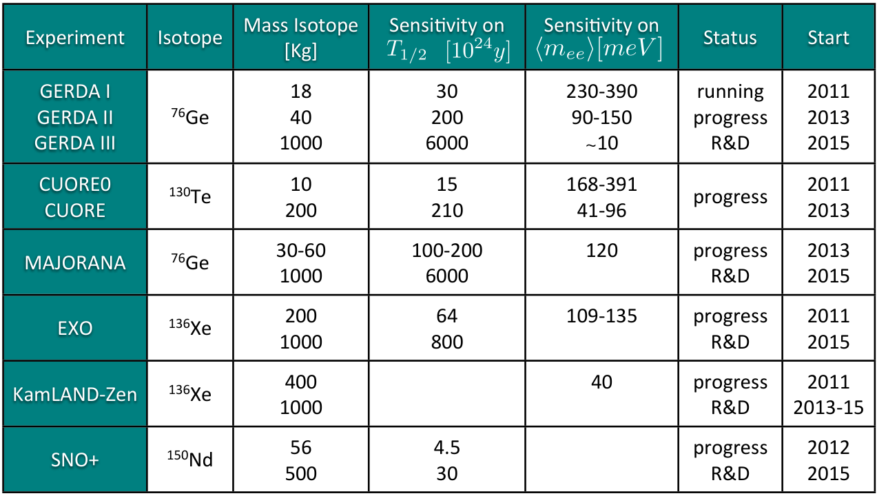
An incomplete list of current and future experiments is presented in fig. 3.2(b): all the experiments have been designed to reach and pass the H-M claim and the first results are expected in few years. Furthermore, notice that many different techniques and many different isotopes are involved in these list: this will allow the determination of the systematic errors, a better understanding of signals and backgrounds and possibly the discrimination among different mechanisms originating the $0\nu 2\beta$ decay.

The experimental results of the $0\nu 2\beta$ half-time is translated into particle physics parameters by the following expression:

where $G^{0\nu}(Q^{5},Z)$ is the phase space, $M^{0\nu}(A,Z)$ the matrix element and $\Pi$ is a function of particle physics parameters. The phase space may depend on the particle physics process that determines the $0\nu 2\beta$ decay, but it is almost equal for transitions with only 2 electrons in the final state, as can be noticed in fig. 3.3(a).

The nuclear matrix element $M^{0\nu}(A,Z)$ depends on the particle physics process which determines the transitions and on the isotope considered. Two main approaches are followed: the Nuclear Shell Model (NSM) allows the study of arbitrary complicated configurations, but limited to few single-particle orbitals outside the inert core; the Quasi-particle Random Phase Approximation (QRPS) is able to treat many single-particle states, but only a limited set of configurations. In fig. 3.3(b) we can see the results of the two methods for different isotopes. To be noticed that a lot of effort has been put for the Standard mechanism, but not for the exotic ones. It is from the nuclear matrix element computations that comes the largest theoretical uncertainty in the $0\nu 2\beta$ decay rate and unfortunately the precision is not expected to improve more that $20\%$ in the next 10 years.

Bibliography

- [1] G. L. Fogli, E. Lisi, A. Marrone, A. Palazzo and A. M. Rotunno, Phys. Rev. D 84 (2011) 053007 [arXiv:1106.6028 [hep-ph]].
- [2] G. L. Fogli, E. Lisi, A. Marrone, A. Melchiorri, A. Palazzo, A. M. Rotunno, P. Serra and J. Silk et al., Phys. Rev. D 78 (2008) 033010 [arXiv:0805.2517 [hep-ph]].
- [3] J. J. Gomez-Cadenas, J. Martin-Albo, M. Mezzetto, F. Monrabal and M. Sorel, arXiv:1109.5515 [hep-ex].
- [4] C. Kraus, B. Bornschein, L. Bornschein, J. Bonn, B. Flatt, A. Kovalik, B. Ostrick and E. W. Otten et al., Eur. Phys. J. C 40 (2005) 447 [hep-ex/0412056]; V. M. Lobashev, Nucl. Phys. A 719 (2003) 153.
- [5] K. Abe et al. [T2K Collaboration], Phys. Rev. Lett. 107 (2011) 041801. [arXiv:1106.2822 [hep-ex]].
- [6] T. Fukuyama and H. Nishiura, hep-ph/9702253; E. Ma and M. Raidal, Phys. Rev. Lett. 87 (2001) 011802 [Erratum-ibid. 87 (2001) 159901] [hep-ph/0102255]; C. S. Lam, Phys. Lett. B 507 (2001) 214 [hep-ph/0104116].
- [7] P. F. Harrison, D. H. Perkins and W. G. Scott, Phys. Lett. B 530 (2002) 167 [arXiv:hep-ph/0202074]; P. F. Harrison and W. G. Scott, Phys. Lett. B 535 (2002) 163 [arXiv:hep-ph/0203209]; Z. z. Xing, Phys. Lett. B 533 (2002) 85 [arXiv:hep-ph/0204049].
- [8] A. Datta, F. -S. Ling and P. Ramond, Nucl. Phys. B 671 (2003) 383 [hep-ph/0306002]; Y. Kajiyama, M. Raidal and A. Strumia, Phys. Rev. D 76 (2007) 117301 [arXiv:0705.4559 [hep-ph]].
- [9] V. D. Barger, S. Pakvasa, T. J. Weiler and K. Whisnant, Phys. Lett. B 437 (1998) 107 [hep-ph/9806387]; R. N. Mohapatra and S. Nussinov, Phys. Rev. D 60 (1999) 013002 [hep-ph/9809415]; G. Altarelli and F. Feruglio, JHEP 9811 (1998) 021 [hep-ph/9809596].
- [10] R. Barbieri and L. J. Hall, Nuovo Cim. A 110 (1997) 1 [hep-ph/9605224]; R. Barbieri, L. J. Hall, S. Raby and A. Romanino, Nucl. Phys. B 493 (1997) 3 [hep-ph/9610449]; R. Barbieri, L. J. Hall and A. Romanino, Phys. Lett. B 401 (1997) 47 [hep-ph/9702315].
- [11] S. F. King, JHEP 0508 (2005) 105 [hep-ph/0506297].
- [12] S. F. King and G. G. Ross, Phys. Lett. B 520 (2001) 243 [hep-ph/0108112]; Phys. Lett. B 574 (2003) 239 [hep-ph/0307190].
- [13] I. de Medeiros Varzielas, S. F. King and G. G. Ross, Phys. Lett. B 644 (2007) 153 [hep-ph/0512313]; S. F. King and M. Malinsky, Phys. Lett. B 645 (2007) 351 [hep-ph/0610250].
- [14] G. Altarelli and F. Feruglio, Nucl. Phys. B 741 (2006) 215 [arXiv:hep-ph/0512103].
- [15] F. Feruglio, C. Hagedorn, Y. Lin and L. Merlo, Nucl. Phys. B 775 (2007) 120 [Erratum-ibid. 836 (2010) 127] [arXiv:hep-ph/0702194].
- [16] C. S. Lam, Phys. Lett. B 656 (2007) 193 [arXiv:0708.3665 [hep-ph]]; Phys. Rev. Lett. 101 (2008) 121602 [arXiv:0804.2622 [hep-ph]]; Phys. Rev. D 78 (2008) 073015 [arXiv:0809.1185 [hep-ph]].
- [17] C. Hagedorn and M. Serone, JHEP 1110 (2011) 083 [arXiv:1106.4021 [hep-ph]].
- [18] Y. Lin, Nucl. Phys. B 824 (2010) 95 [arXiv:0905.3534 [hep-ph]].
- [19] G. Altarelli, F. Feruglio and L. Merlo, JHEP 0905 (2009) 020 [arXiv:0903.1940 [hep-ph]].
- [20] A. Blum, C. Hagedorn and M. Lindner, Phys. Rev. D 77 (2008) 076004 [arXiv:0709.3450 [hep-ph]].
- [21] A. Adulpravitchai, A. Blum and C. Hagedorn, JHEP 0903 (2009) 046 [arXiv:0812.3799 [hep-ph]]; C. Hagedorn and R. Ziegler, Phys. Rev. D 82 (2010) 053011 [arXiv:1007.1888 [hep-ph]].
- [22] A. Blum and C. Hagedorn, Nucl. Phys. B 821 (2009) 327 [arXiv:0902.4885 [hep-ph]].
- [23] C. Hagedorn and D. Meloni, in preparation.
Chapter 3 Neutrinoless Double Beta Decay and Connections with Flavour Physics
Luca Merlo
Abstract
Neutrinoless double beta () decay is a fundamental observable to probe the Majorana character of neutrinos and to investigate on their absolute mass scale. The present status of experiments searching for decay is reviewed and the most relevant results are discussed. The interplay with flavour physics in general provides clear predictions for decay and some major examples are presented.
3.1 Introduction
- [1] T. Schwetz, M. Tortola, and J. W. F. Valle, arXiv: 1108.1376.
- [2] J. Schechter and J. W. F. Valle, Phys. Rev. D25 (1982) 2951.
- [3] M. Hirsch, S. Kovalenko, and I. Schmidt, Phys. Lett. B642 (2006) 106–110 [arXiv: hep-ph/0608207].
- [4] W. Rodejohann, arXiv: 1106.1334.
- [5] H. V. Klapdor-Kleingrothaus et al., Eur. Phys. J. A12 (2001) 147–154 [arXiv: hep-ph/0103062].
- [6] H. V. Klapdor-Kleingrothaus and I. V. Krivosheina, Mod. Phys. Lett. A21 (2006) 1547–1566.
- [7] M. C. Gonzalez-Garcia, M. Maltoni, and J. Salvado, JHEP 08 (2010) 117 [arXiv: 1006.3795].
- [8] C. Kraus et al., Eur. Phys. J. C40 (2005) 447–468 [arXiv: hep-ex/0412056].
- [9] V. M. Lobashev, Nucl. Phys. A719 (2003) 153–160.
- [10] O. Host, O. Lahav, F. B. Abdalla, and K. Eitel, Phys. Rev. D76 (2007) 113005 [arXiv: 0709.1317].
- [11] A. Monfardini et al., Nucl. Instrum. Meth. A559 (2006) 346–348 [arXiv: hep-ex/0509038].
- [12] G. L. Fogli, E. Lisi, A. Marrone, A. Palazzo, and A. M. Rotunno, arXiv: 1106.6028.
- [13] See the contribution by W. Rodejohann on this conference proceeding.
- [14] P. F. Harrison, D. H. Perkins, and W. G. Scott, Phys. Lett. B530 (2002) 167 [arXiv: hep-ph/0202074].
- [15] Z.-z. Xing, Phys. Lett. B533 (2002) 85–93 [arXiv: hep-ph/0204049].
- [16] V. D. Barger, S. Pakvasa, T. J. Weiler, and K. Whisnant, Phys. Lett. B437 (1998) 107–116 [arXiv: hep-ph/9806387].
- [17] G. Altarelli and F. Feruglio, JHEP 11 (1998) 021 [arXiv: hep-ph/9809596].
- [18] Y. Kajiyama, M. Raidal, and A. Strumia, Phys. Rev. D76 (2007) 117301 [arXiv: 0705.4559].
- [19] W. Rodejohann, Phys. Lett. B671 (2009) 267–271 [arXiv: 0810.5239].
- [20] G. Altarelli, F. Feruglio, and L. Merlo, JHEP 05 (2009) 020 [arXiv: 0903.1940].
- [21] R. de Adelhart Toorop, F. Bazzocchi, and L. Merlo, JHEP 08 (2010) 001 [arXiv: 1003.4502].
- [22] D. Meloni, arXiv: 1107.0221.
- [23] See the contributions by C. Hagedorn and F. Bazzocchi on this conference proceeding.
- [24] G. Altarelli and F. Feruglio, Nucl. Phys. B741 (2006) 215–235 [arXiv: hep-ph/0512103].
- [25] G. Altarelli and F. Feruglio, Nucl. Phys. B720 (2005) 64–88 [arXiv: hep-ph/0504165].
- [26] F. Feruglio, C. Hagedorn, Y. Lin, and L. Merlo, Nucl. Phys. B775 (2007) 120–142 [arXiv: hep-ph/0702194].
- [27] M. Hirsch, S. Morisi, and J. W. F. Valle, Phys. Rev. D78 (2008) 093007 [arXiv: 0804.1521].
- [28] F. Bazzocchi, L. Merlo, and S. Morisi, Phys. Rev. D80 (2009) 053003 [arXiv: 0902.2849].
- [29] F. Bazzocchi, L. Merlo, and S. Morisi, Nucl. Phys. B816 (2009) 204–226 [arXiv: 0901.2086].
- [30] F. Feruglio, C. Hagedorn, Y. Lin, and L. Merlo, Nucl. Phys. B809 (2009) 218–243 [arXiv: 0807.3160].
- [31] F. Feruglio, C. Hagedorn, and L. Merlo, JHEP 03 (2010) 084 [arXiv: 0910.4058].
- [32] Y. Lin, L. Merlo, and A. Paris, Nucl. Phys. B835 (2010) 238–261 [arXiv: 0911.3037].
- [33] F. Feruglio, C. Hagedorn, Y. Lin, and L. Merlo, Nucl. Phys. B832 (2010) 251–288 [arXiv: 0911.3874].
- [34] C. Hagedorn, E. Molinaro, and S. T. Petcov, JHEP 02 (2010) 047 [arXiv: 0911.3605].
- [35] L. Merlo, S. Rigolin, and B. Zaldivar, arXiv: 1108.1795.
- [36] E. Bertuzzo, P. Di Bari, F. Feruglio, and E. Nardi, JHEP 11 (2009) 036 [arXiv: 0908.0161].
- [37] D. Aristizabal Sierra, F. Bazzocchi, I. de Medeiros Varzielas, L. Merlo, and S. Morisi, Nucl. Phys. B827 (2010) 34–58 [arXiv: 0908.0907].
- [38] C. Hagedorn, E. Molinaro, and S. T. Petcov, JHEP 09 (2009) 115 [arXiv: 0908.0240].
Chapter 4 Deviations and alternatives to tri-bimaximal mixing
Werner Rodejohann
The overwhelming majority of flavor symmetry models focusses on tri-bimaximal mixing (TBM). Neutrino mass sum-rules are given as one rather robust example on how to distinguish some of the models from each other. We classify mechanisms to deviate from TBM and estimate the typical order of magnitude of the corrections. Then we present several alternatives to TBM, and outline their possible origin in flavor symmetries. Finally, examples on how to to accommodate light sterile neutrinos in flavor symmetry model are discussed. This works for eV-scale sterile neutrinos to explain the reactor anomaly, as well as for keV-scale sterile neutrinos which can act as warm dark matter.
4.1 Introduction: The Zoo of Models and how to distinguish them
There is no need here to motivate the need for flavor symmetry models, or to note the existence of a huge amount of those, for reviews see [1]. The vast majority aims to reproduce tri-bimaximal mixing (TBM),
- [1] G. Altarelli and F. Feruglio, Rev. Mod. Phys. 82 (2010) 2701 [arXiv:1002.0211 [hep-ph]]; H. Ishimori et al., Prog. Theor. Phys. Suppl. 183 (2010) 1 [arXiv:1003.3552 [hep-th]].
- [2] J. Barry and W. Rodejohann, Phys. Rev. D 81 (2010) 093002 [Erratum-ibid. D 81 (2010) 119901] [arXiv:1003.2385 [hep-ph]].
- [3] J. Barry and W. Rodejohann, Nucl. Phys. B 842 (2011) 33 [arXiv:1007.5217 [hep-ph]].
- [4] L. Dorame, D. Meloni, S. Morisi, E. Peinado and J. W. F. Valle, arXiv:1111.5614 [hep-ph].
- [5] R. Allahverdi, B. Dutta and R. N. Mohapatra, Phys. Lett. B 695 (2011) 181 [arXiv:1008.1232 [hep-ph]]; J. Barry, R. N. Mohapatra and W. Rodejohann, Phys. Rev. D 83 (2011) 113012 [arXiv:1012.1761 [hep-ph]]; S. Morisi and E. Peinado, Phys. Lett. B 701 (2011) 451 [arXiv:1104.4961 [hep-ph]].
- [6] M. Hirsch, S. Morisi and J. W. F. Valle, Phys. Rev. D 78 (2008) 093007 [arXiv:0804.1521 [hep-ph]].
- [7] W. Rodejohann, Int. J. Mod. Phys. E 20 (2011) 1833 [arXiv:1106.1334 [hep-ph]].
- [8] K. Abe et al. [T2K Collaboration], Phys. Rev. Lett. 107 (2011) 041801 [arXiv:1106.2822 [hep-ex]].
- [9] H. de Kerret, talk at LowNu, Seoul (Korea), Nov. 6 2011, for the slides see http://workshop.kias.re.kr/lownu11/?Program
- [10] S. Goswami, S. T. Petcov, S. Ray and W. Rodejohann, Phys. Rev. D 80 (2009) 053013 [arXiv:0907.2869 [hep-ph]].
- [11] M. Abbas and A. Yu. .Smirnov, Phys. Rev. D 82 (2010) 013008 [arXiv:1004.0099 [hep-ph]].
- [12] R. d. A. Toorop, F. Feruglio and C. Hagedorn, Phys. Lett. B 703 (2011) 447 [arXiv:1107.3486 [hep-ph]].
- [13] W. Rodejohann, H. Zhang and S. Zhou, Nucl. Phys. B 855 (2012) 592 [arXiv:1107.3970 [hep-ph]].
- [14] F. Bazzocchi, arXiv:1108.2497 [hep-ph].
- [15] S. Pakvasa, W. Rodejohann and T. J. Weiler, Phys. Rev. Lett. 100 (2008) 111801 [arXiv:0711.0052 [hep-ph]].
- [16] M. Raidal, Phys. Rev. Lett. 93 (2004) 161801 [hep-ph/0404046]; H. Minakata and A. Yu. .Smirnov, Phys. Rev. D 70 (2004) 073009 [hep-ph/0405088].
- [17] A. Dighe, S. Goswami and P. Roy, Phys. Rev. D 76 (2007) 096005 [arXiv:0704.3735 [hep-ph]]; A. Dighe, S. Goswami and W. Rodejohann, Phys. Rev. D 75 (2007) 073023 [hep-ph/0612328].
- [18] C. H. Albright and W. Rodejohann, Phys. Lett. B 665 (2008) 378 [arXiv:0804.4581 [hep-ph]].
- [19] M. Honda and M. Tanimoto, Prog. Theor. Phys. 119 (2008) 583 [arXiv:0801.0181 [hep-ph]].
- [20] G. Altarelli, F. Feruglio and L. Merlo, JHEP 0905 (2009) 020 [arXiv:0903.1940 [hep-ph]].
- [21] Y. Lin, Nucl. Phys. B 824 (2010) 95 [arXiv:0905.3534 [hep-ph]].
- [22] C. Hagedorn and R. Ziegler, Phys. Rev. D 82 (2010) 053011 [arXiv:1007.1888 [hep-ph]].
- [23] H. Ishimori, K. Saga, Y. Shimizu and M. Tanimoto, Phys. Rev. D 81 (2010) 115009 [arXiv:1004.5004 [hep-ph]].
- [24] C. H. Albright, A. Dueck and W. Rodejohann, Eur. Phys. J. C 70 (2010) 1099 [arXiv:1004.2798 [hep-ph]].
- [25] A. Datta, F. -S. Ling and P. Ramond, Nucl. Phys. B 671 (2003) 383 [hep-ph/0306002]; Y. Kajiyama, M. Raidal and A. Strumia, Phys. Rev. D 76 (2007) 117301 [arXiv:0705.4559 [hep-ph]].
- [26] L. L. Everett and A. J. Stuart, Phys. Rev. D 79 (2009) 085005 [arXiv:0812.1057 [hep-ph]]; Phys. Lett. B 698 (2011) 131 [arXiv:1011.4928 [hep-ph]]; G. -J. Ding, L. L. Everett and A. J. Stuart, arXiv:1110.1688 [hep-ph].
- [27] F. Feruglio and A. Paris, JHEP 1103 (2011) 101 [arXiv:1101.0393 [hep-ph]].
- [28] W. Rodejohann, Phys. Lett. B 671 (2009) 267 [arXiv:0810.5239 [hep-ph]]; A. Adulpravitchai, A. Blum and W. Rodejohann, New J. Phys. 11 (2009) 063026 [arXiv:0903.0531 [hep-ph]].
- [29] A. Blum, C. Hagedorn and A. Hohenegger, JHEP 0803 (2008) 070 [arXiv:0710.5061 [hep-ph]].
- [30] J. E. Kim and M. -S. Seo, JHEP 1102 (2011) 097 [arXiv:1005.4684 [hep-ph]].
- [31] T. Schwetz, M. Tortola and J. W. F. Valle, New J. Phys. 13 (2011) 109401 [arXiv:1108.1376 [hep-ph]].
- [32] W. Grimus and L. Lavoura, JHEP 0809 (2008) 106 [arXiv:0809.0226 [hep-ph]]; C. H. Albright and W. Rodejohann, Eur. Phys. J. C 62 (2009) 599 [arXiv:0812.0436 [hep-ph]]; W. Grimus, L. Lavoura and A. Singraber, Phys. Lett. B 686 (2010) 141 [arXiv:0911.5120 [hep-ph]]; X. -G. He and A. Zee, Phys. Rev. D 84 (2011) 053004 [arXiv:1106.4359 [hep-ph]].
- [33] Z. -z. Xing, Phys. Rev. D 78 (2008) 011301 [arXiv:0805.0416 [hep-ph]].
- [34] S. F. King, Phys. Lett. B 675 (2009) 347 [arXiv:0903.3199 [hep-ph]].
- [35] T. Kitabayashi and M. Yasue, Phys. Lett. B 696 (2011) 478 [arXiv:1101.2073 [hep-ph]].
- [36] S. Morisi, K. M. Patel and E. Peinado, Phys. Rev. D 84 (2011) 053002 [arXiv:1107.0696 [hep-ph]].
- [37] P. A. N. Machado, H. Minakata, H. Nunokawa and R. Z. Funchal, arXiv:1111.3330 [hep-ph].
- [38] G. Altarelli and F. Feruglio, Nucl. Phys. B 720 (2005) 64 [hep-ph/0504165]; Nucl. Phys. B 741 (2006) 215 [arXiv:hep-ph/0512103].
- [39] C. S. Lam, Phys. Rev. Lett. 101 (2008) 121602 [arXiv:0804.2622 [hep-ph]]; W. Grimus, L. Lavoura and P. O. Ludl, J. Phys. GG 36 (2009) 115007 [arXiv:0906.2689 [hep-ph]].
- [40] S. -F. Ge, H. -J. He and F. -R. Yin, JCAP 1005 (2010) 017 [arXiv:1001.0940 [hep-ph]]; D. A. Dicus, S. -F. Ge and W. W. Repko, Phys. Rev. D 83 (2011) 093007 [arXiv:1012.2571 [hep-ph]]; Phys. Lett. B 702 (2011) 220 [arXiv:1104.0602 [hep-ph]]; H. -J. He and F. -R. Yin, Phys. Rev. D 84 (2011) 033009 [arXiv:1104.2654 [hep-ph]]. J. Heeck and W. Rodejohann, arXiv:1112.3628 [hep-ph].
- [41] G. Mention et al., Phys. Rev. D 83 (2011) 073006 [arXiv:1101.2755 [hep-ex]]; P. Huber, Phys. Rev. C 84 (2011) 024617 [arXiv:1106.0687 [hep-ph]].
- [42] J. Kopp, M. Maltoni and T. Schwetz, Phys. Rev. Lett. 107 (2011) 091801 [arXiv:1103.4570 [hep-ph]]; C. Giunti and M. Laveder, Phys. Rev. D 84 (2011) 073008 [arXiv:1107.1452 [hep-ph]].
- [43] R. H. Cyburt et al., Astropart. Phys. 23 (2005) 313 [astro-ph/0408033]; Y. I. Izotov and T. X. Thuan, Astrophys. J. 710 (2010) L67 [arXiv:1001.4440 [astro-ph.CO]]; J. Hamann et al., Phys. Rev. Lett. 105 (2010) 181301 [arXiv:1006.5276 [hep-ph]]; E. Giusarmaet al., Phys. Rev. D 83 (2011) 115023 [arXiv:1102.4774 [astro-ph.CO]].
- [44] J. Hamann et al., JCAP 1109 (2011) 034 [arXiv:1108.4136 [astro-ph.CO]].
- [45] J. Beun et al., Phys. Rev. D 73 (2006) 093007 [hep-ph/0602012]; I. Tamborra et al., arXiv:1110.2104 [astro-ph.SR].
- [46] J. Barry, W. Rodejohann and H. Zhang, JHEP 1107 (2011) 091 [arXiv:1105.3911 [hep-ph]].
- [47] J. Barry, W. Rodejohann and H. Zhang, arXiv:1110.6382 [hep-ph].
- [48] H. J. de Vega and N. G. Sanchez, arXiv:1109.3187 [astro-ph.CO].
- [49] M. Shaposhnikov, Nucl. Phys. B 763 (2007) 49 [hep-ph/0605047]; M. Lindner, A. Merle and V. Niro, JCAP 1101 (2011) 034 [arXiv:1011.4950 [hep-ph]]; A. Merle and V. Niro, JCAP 1107 (2011) 023 [arXiv:1105.5136 [hep-ph]]; A. Kusenko, F. Takahashi and T. T. Yanagida, Phys. Lett. B 693 (2010) 144 [arXiv:1006.1731 [hep-ph]]; A. Adulpravitchai and R. Takahashi, JHEP 1109 (2011) 127 [arXiv:1107.3829 [hep-ph]]; H. Zhang, arXiv:1110.6838 [hep-ph].
- [50] M. Hirsch, S. Morisi, E. Peinado and J. W. F. Valle, Phys. Rev. D 82 (2010) 116003 [arXiv:1007.0871 [hep-ph]]; M. S. Boucenna et al., JHEP 1105 (2011) 037 [arXiv:1101.2874 [hep-ph]].
Chapter 5 News on indirect and direct dark matter searches
Marco Taoso
We review the current status of direct and indirect Dark Matter searches, focusing in particular on those observations which have been interpreted as possible hints of dark matter. We discuss about the uncertainties affecting these interpretations and highlights the complementarity between different methods.
5.1 Introduction
Non-baryonic Dark Matter is a fundamental pillar of modern cosmology [1]. Astrophysical and cosmological observations have probed its presence from subgalactic up to cosmological scales and demonstrated that DM constitutes the most abundant component of the matter budget of the Universe. Furthermore, the increasing amount of data collected over the last decades have constrained its fundamental properties. The emergent picture is that DM is made up of cold (or warm) massive particles, stable over cosmological times and interacting only (very) weakly with the primordial plasma of the Universe (see Ref.[2] for a review about the properties that a viable dark matter candidate should have). Particles fulfilling these requirements arise in many extensions of the Standard Model (SM) of the particle physics, motivating the connection of the DM problem with searches of new physics beyond the SM.
Presently, the nature of DM remains elusive and its microscopic properties are still undetermined. To shed light on this mistery it is needed to go beyond a gravitational detection of DM. High-energy colliders are ideal tools to search for new particles and interactions. Since DM should interacts only weakly, it is expected to be invisible to the detectors exploited at collider experiments, and therefore it should manifest itself as missing energy events. This is an exciting time for searches of new physics. Indeed, the Large Hadron Collider (LHC) is currently taking data, probing energies previously unexplored at colliders. However, in case that a potential DM candidate will be discovered at LHC, additional information will be mandatory to demonstrate that this new particle constitutes the DM component observed with cosmological and astrophysical observations. Measuring the mass and the interaction cross sections of this particle might allow to reconstruct its cosmological relic density and to compare this estimate with the DM abundance inferred from cosmlogical observations. This will probably be very difficult to do only with the information obtained at LHC [3, 5]. Furthermore, this calculation would involve cosmological assumptions on the evolution of the Universe.
Direct and Indirect DM searches provide alternative strategies to search for non-gravitational DM signals. Direct detection experiments looks for the interaction of DM particles with low-background dectors. These searches are mainly devoted to look for DM in the form of Weakly Interacting Massive particles (WIMPs), i.e. DM candidates with masses in the GeV-TeV range and interaction strenghts of the order of those mediated by weak interactions. WIMPs are predicted in many extensions of the Standard Model, in particular those related with the electroweak hierarchy problem, like Supersymmetry and extra-dimension models. These particles were in thermal equilibrium with the plasma in the early Universe and decoupled non-relativistically, inheriting the correct relic abundance for an annihilation cross-section a value typical for weak-scale interactions. The detection of the WIMPs annihilation products is alternative indirect method to look for WIMPs, or more in general to search for any DM candidate with sizeable annihilations or decays into SM particles.
In the following, we will focus on direct and indirect DM searches. We will review the present status and discuss the future prospects for detection.
5.2 Direct Detection
Direct DM searches aim at detecting DM particles through the measurement of nuclear recoils produced by DM scattering off target nuclei (see [6] for a recent review). The differential rate in events/kg/day/keV is given by:
- [1] G. Bertone, (ed.), Cambridge, UK: Univ. Pr. (2010) 738 p
- [2] M. Taoso, G. Bertone and A. Masiero, JCAP 0803 (2008) 022 [arXiv:0711.4996 [astro-ph]].
- [3] E. A. Baltz, M. Battaglia, M. E. Peskin and T. Wizansky, Phys. Rev. D 74 (2006) 103521 [hep-ph/0602187].
- [4] G. Bertone, D. G. Cerdeno, M. Fornasa, R. R. de Austri and R. Trotta, Phys. Rev. D 82 (2010) 055008 [arXiv:1005.4280 [hep-ph]].
- [5] G. Bertone, D. G. Cerdeno, M. Fornasa, L. Pieri, R. R. de Austri and R. Trotta, arXiv:1111.2607 [astro-ph.HE].
- [6] D. G. Cerdeno, A. M. Green, In *Bertone, G. (ed.): Particle dark matter* 347-369. [arXiv:1002.1912 [astro-ph.CO]].
- [7] R. Bernabei et al. [ DAMA Collaboration ], Eur. Phys. J. C56 (2008) 333-355. [arXiv:0804.2741 [astro-ph]].
- [8] C. E. Aalseth et al. [ CoGeNT Collaboration ], Phys. Rev. Lett. 106 (2011) 131301. [arXiv:1002.4703 [astro-ph.CO]].
- [9] C. E. Aalseth, P. S. Barbeau, J. Colaresi, J. I. Collar, J. Diaz Leon, J. E. Fast, N. Fields, T. W. Hossbach et al., Phys. Rev. Lett. 107 (2011) 141301. [arXiv:1106.0650 [astro-ph.CO]].
- [10] G. Angloher, M. Bauer, I. Bavykina, A. Bento, C. Bucci, C. Ciemniak, G. Deuter, F. von Feilitzsch et al., [arXiv:1109.0702 [astro-ph.CO]].
- [11] T. Schwetz, J. Zupan, JCAP 1108 (2011) 008. [arXiv:1106.6241 [hep-ph]].
- [12] J. Kopp, T. Schwetz, J. Zupan, [arXiv:1110.2721 [hep-ph]].
- [13] M. Farina, D. Pappadopulo, A. Strumia, T. Volansky, JCAP 1111 (2011) 010. [arXiv:1107.0715 [hep-ph]].
- [14] C. Kelso, D. Hooper, M. R. Buckley, [arXiv:1110.5338 [astro-ph.CO]].
- [15] E. Del Nobile, C. Kouvaris, F. Sannino, J. Virkajarvi, [arXiv:1111.1902 [hep-ph]].
- [16] N. Fornengo, P. Panci, M. Regis, [arXiv:1108.4661 [hep-ph]].
- [17] C. Savage, G. Gelmini, P. Gondolo, K. Freese, Phys. Rev. D83 (2011) 055002. [arXiv:1006.0972 [astro-ph.CO]].
- [18] C. Arina, J. Hamann, R. Trotta, Y. Y. YWong, [arXiv:1111.3238 [hep-ph]].
- [19] D. Tucker-Smith, N. Weiner, Phys. Rev. D64 (2001) 043502. [hep-ph/0101138].
- [20] E. Del Nobile, C. Kouvaris, F. Sannino, Phys. Rev. D84 (2011) 027301. [arXiv:1105.5431 [hep-ph]].
- [21] S. Chang, J. Liu, A. Pierce, N. Weiner, I. Yavin, JCAP 1008 (2010) 018. [arXiv:1004.0697 [hep-ph]].
- [22] S. Chang, A. Pierce, N. Weiner, JCAP 1001 (2010) 006. [arXiv:0908.3192 [hep-ph]].
- [23] Y. Bai, P. J. Fox, JHEP 0911 (2009) 052. [arXiv:0909.2900 [hep-ph]].
- [24] E. Aprile et al. [ XENON100 Collaboration ], Phys. Rev. Lett. 107 (2011) 131302. [arXiv:1104.2549 [astro-ph.CO]].
- [25] Z. Ahmed et al. [ CDMS-II Collaboration ], Phys. Rev. Lett. 106 (2011) 131302. [arXiv:1011.2482 [astro-ph.CO]].
- [26] D. S. Akerib et al. [ CDMS Collaboration ], Phys. Rev. Lett. 96 (2006) 011302. [astro-ph/0509259].
- [27] J. I. Collar, [arXiv:1106.0653 [astro-ph.CO]].
- [28] J. I. Collar, [arXiv:1010.5187 [astro-ph.IM]].
- [29] T. X. Collaboration, arXiv:1005.2615 [astro-ph.CO].
- [30] G. Plante, E. Aprile, R. Budnik, B. Choi, K. L. Giboni, L. W. Goetzke, R. F. Lang, K. E. Lim et al., Phys. Rev. C84 (2011) 045805. [arXiv:1104.2587 [nucl-ex]].
- [31] C. Savage, K. Freese, P. Gondolo, D. Spolyar, JCAP 0909 (2009) 036. [arXiv:0901.2713 [astro-ph]].
- [32] T. F. -L. collaboration, [arXiv:1108.3546 [astro-ph.HE]].
- [33] A. A. Abdo et al. [ The Fermi-LAT Collaboration ], Phys. Rev. Lett. 104 (2010) 101101. [arXiv:1002.3603 [astro-ph.HE]].
- [34] A. A. Abdo et al. [ Fermi-LAT Collaboration ], JCAP 1004 (2010) 014. [arXiv:1002.4415 [astro-ph.CO]].
- [35] S. ’i. Ando, E. Komatsu, T. Narumoto, T. Totani, Phys. Rev. D75 (2007) 063519. [astro-ph/0612467].
- [36] M. Fornasa, L. Pieri, G. Bertone, E. Branchini, Phys. Rev. D80 (2009) 023518. [arXiv:0901.2921 [astro-ph]].
- [37] J. M. Siegal-Gaskins, JCAP 0810 (2008) 040. [arXiv:0807.1328 [astro-ph]].
- [38] M. Taoso, S. ’i. Ando, G. Bertone, S. Profumo, Phys. Rev. D79 (2009) 043521. [arXiv:0811.4493 [astro-ph]].
- [39] A. Cuoco, A. Sellerholm, J. Conrad, S. Hannestad, Mon. Not. Roy. Astron. Soc. 414 (2011) 2040-2054. [arXiv:1005.0843 [astro-ph.HE]].
- [40] A. Cuoco, T. Linden, M. N. Mazziotta, J. M. Siegal-Gaskins, V. Vitale, f. t. F. -L. Collaboration, E. Komatsu, [arXiv:1110.1047 [astro-ph.HE]].
- [41] M. Fornasa, J. Zavala, M. A. Sanchez-Conde, F. Prada, M. Vogelsberger, [arXiv:1110.0324 [astro-ph.CO]].
- [42] A. Abramowski et al. [ H.E.S.S. Collaboration ], Phys. Rev. Lett. 106 (2011) 161301. [arXiv:1103.3266 [astro-ph.HE]].
- [43] M. Su, T. R. Slatyer, D. P. Finkbeiner, Astrophys. J. 724 (2010) 1044-1082. [arXiv:1005.5480 [astro-ph.HE]].
- [44] G. Dobler, I. Cholis, N. Weiner, Astrophys. J. 741 (2011) 25. [arXiv:1102.5095 [astro-ph.HE]].
- [45] D. Hooper, T. Linden, [arXiv:1110.0006 [astro-ph.HE]].
- [46] A. Boyarsky, D. Malyshev, O. Ruchayskiy, Phys. Lett. B705 (2011) 165-169. [arXiv:1012.5839 [hep-ph]].
- [47] M. Chernyakova, D. Malyshev, F. A. Aharonian, R. M. Crocker, D. I. Jones, Astrophys. J. 726 (2011) 60. [arXiv:1009.2630 [astro-ph.HE]].
- [48] D. Hooper, T. Linden, [arXiv:1110.0006 [astro-ph.HE]].
- [49] A. Boyarsky, D. Malyshev, O. Ruchayskiy, Phys. Lett. B705 (2011) 165-169. [arXiv:1012.5839 [hep-ph]].
- [50] M. Chernyakova, D. Malyshev, F. A. Aharonian, R. M. Crocker, D. I. Jones, Astrophys. J. 726 (2011) 60. [arXiv:1009.2630 [astro-ph.HE]].
- [51] Y. Mambrini, JCAP 0912 (2009) 005. [arXiv:0907.2918 [hep-ph]].
- [52] C. B. Jackson, G. Servant, G. Shaughnessy, T. M. P. Tait, M. Taoso, JCAP 1004 (2010) 004. [arXiv:0912.0004 [hep-ph]].
- [53] G. Bertone, C. B. Jackson, G. Shaughnessy, T. M. P. Tait, A. Vallinotto, Phys. Rev. D80 (2009) 023512. [arXiv:0904.1442 [astro-ph.HE]].
- [54] M. Garny, A. Ibarra, D. Tran, C. Weniger, JCAP 1101 (2011) 032. [arXiv:1011.3786 [hep-ph]].
- [55] A. A. Abdo, M. Ackermann, M. Ajello, W. B. Atwood, L. Baldini, J. Ballet, G. Barbiellini, D. Bastieri et al., Phys. Rev. Lett. 104 (2010) 091302. [arXiv:1001.4836 [astro-ph.HE]].
- [56] G. Vertongen, C. Weniger, JCAP 1105 (2011) 027. [arXiv:1101.2610 [hep-ph]].
- [57] X. Huang, G. Vertongen, C. Weniger, [arXiv:1110.6236 [astro-ph.HE]].
- [58] D. Restrepo, M. Taoso, J. W. F. Valle, O. Zapata, [arXiv:1109.0512 [hep-ph]].
- [59] G. A. Gomez-Vargas, M. Fornasa, F. Zandanel, A. J. Cuesta, C. Munoz, F. Prada, G. Yepes, [arXiv:1110.3305 [astro-ph.HE]].
- [60] T. Bringmann, F. Calore, G. Vertongen and C. Weniger, arXiv:1106.1874 [hep-ph].
- [61] O. Adriani et al. [PAMELA Collaboration], Nature 458 (2009) 607 [arXiv:0810.4995 [astro-ph]].
- [62] , et al. [The Fermi LAT Collaboration], arXiv:1109.0521 [astro-ph.HE].
- [63] P. D. Serpico, arXiv:1108.4827 [astro-ph.HE].
- [64] G. Bertone, M. Cirelli, A. Strumia and M. Taoso, JCAP 0903 (2009) 009 [arXiv:0811.3744 [astro-ph]].
- [65] L. Bergstrom, G. Bertone, T. Bringmann, J. Edsjo and M. Taoso, Phys. Rev. D 79 (2009) 081303 [arXiv:0812.3895 [astro-ph]].
- [66] P. Meade, M. Papucci, A. Strumia and T. Volansky, Nucl. Phys. B 831 (2010) 178 [arXiv:0905.0480 [hep-ph]].
- [67] L. Dugger, T. E. Jeltema and S. Profumo, JCAP 1012 (2010) 015 [arXiv:1009.5988 [astro-ph.HE]].
- [68] G. Zaharijas et al. [for the Fermi-LAT Collaboration], PoSIDM 2010 (2011) 111 [arXiv:1012.0588 [astro-ph.HE]].
- [69] T. Delahaye, J. Lavalle, R. Lineros, F. Donato and N. Fornengo, Astron. Astrophys. 524 (2010) A51 [arXiv:1002.1910 [astro-ph.HE]].
- [70] E. Borriello, L. Maccione and A. Cuoco, arXiv:1012.0041 [astro-ph.HE].
- [71] F. Donato, N. Fornengo and D. Maurin, Phys. Rev. D 78 (2008) 043506 [arXiv:0803.2640 [hep-ph]].
- [72] Y. Cui, J. D. Mason and L. Randall, JHEP 1011 (2010) 017 [arXiv:1006.0983 [hep-ph]].
- [73] M. Regis and P. Ullio, Phys. Rev. D 78 (2008) 043505 [arXiv:0802.0234 [hep-ph]].
- [74] R. M. Crocker, N. F. Bell, C. Balazs and D. I. Jones, Phys. Rev. D 81 (2010) 063516 [arXiv:1002.0229 [hep-ph]].
- [75] N. Fornengo, R. A. Lineros, M. Regis and M. Taoso, arXiv:1110.4337 [astro-ph.GA].
- [76] D. J. Fixsen, A. Kogut, S. Levin, M. Limon, P. Lubin, P. Mirel, M. Seiffert and J. Singal et al., arXiv:0901.0555 [astro-ph.CO].
- [77] N. Fornengo, R. Lineros, M. Regis and M. Taoso, arXiv:1108.0569 [hep-ph].
- [78] K. Helbing and f. t. I. Collaboration, arXiv:1107.5227 [hep-ex].
- [79] R. Kappl and M. W. Winkler, Nucl. Phys. B 850 (2011) 505 [arXiv:1104.0679 [hep-ph]].
- [80] M. Taoso, F. Iocco, G. Meynet, G. Bertone and P. Eggenberger, Phys. Rev. D 82 (2010) 083509 [arXiv:1005.5711 [astro-ph.CO]].
- [81] D. T. Cumberbatch, J. .A. Guzik, J. Silk, L. S. Watson and S. M. West, Phys. Rev. D 82 (2010) 103503 [arXiv:1005.5102 [astro-ph.SR]].
- [82] M. T. Frandsen and S. Sarkar, Phys. Rev. Lett. 105 (2010) 011301 [arXiv:1003.4505 [hep-ph]].
- [83] D. Spolyar, K. Freese and P. Gondolo, Phys. Rev. Lett. 100 (2008) 051101 [arXiv:0705.0521 [astro-ph]].
- [84] M. Taoso, G. Bertone, G. Meynet and S. Ekstrom, Phys. Rev. D 78 (2008) 123510 [arXiv:0806.2681 [astro-ph]].
- [85] F. Iocco, A. Bressan, E. Ripamonti, R. Schneider, A. Ferrara and P. Marigo, Mon. Not. Roy. Astron. Soc. 390 (2008) 1655 [arXiv:0805.4016 [astro-ph]].
- [86] P. Scott, M. Fairbairn and J. Edsjo, Mon. Not. Roy. Astron. Soc. 394 (2009) 82 [arXiv:0809.1871 [astro-ph]].
- [87] S. D. McDermott, H. -B. Yu and K. M. Zurek, arXiv:1103.5472 [hep-ph].
- [88] C. Kouvaris and P. Tinyakov, Phys. Rev. Lett. 107 (2011) 091301 [arXiv:1104.0382 [astro-ph.CO]].
Chapter 6 Flavored Orbifold GUT – model
Adisorn Adulpravitchai
In this talk, we briefly discuss the idea of flavored orbifold GUT [1], that is, the flavor symmetry might emerge due to orbifold compactification of one orbifold and broken by boundary conditions of another orbifold where the GUT group is broken. The combination of the orbifold parities in gauge and flavor space determines the zero modes. An example of the idea is given in a supersymmetric (SUSY) SO(10) orbifold GUT model, which predicts the tribimaximal mixing at leading order in the lepton sector as well as the Cabibbo angle in the quark sector.
6.1 Introduction
The leptonic mixing matrix is compatible with the tribimaximal mixing matrix [6] and hints towards non-abelian discrete flavor symmetries. However, the origin of a potential flavor symmetry is unclear. As the Standard Model of Particle Physics (SM) is constructed based on the two well-known symmetries, namely, continuous gauge symmetry and space-time symmetry, it is interesting to investigate their origin from these two symmetries.
- •
Extra-dimensions: Non-Abelian discrete symmetries can arise as the remnant symmetry of the broken Poincare (Lorentz) via orbifold compactification on two extra-dimensions. The non-Abelian discrete symmetries are , , , , and [5].
An orbifold compactification of a GUT can lead to its
breaking and nicely solve e.g. the doublet-triplet splitting
problem [6]. Furthermore, the orbifold
compactification can generate the alignment of vacuum expectation values (VEVs)
of flavons [7] transmitting the flavor symmetry breaking
into the fermion mass matrices.
In this talk, we discuss the combination of the origin of a flavor symmetry as
well as its breaking by the VEV alignment of flavons from an orbifold. We
assume two orbifolds, where the flavor symmetry originates from the special
geometry of one orbifold and it is broken on another orbifold. We demonstrate it
with a simple model in the context of a SUSY SO(10) orbifold
GUT with an flavor
symmetry [1] (For , see [8]). The model predicts the tribimaximal mixing at leading order in the lepton sector and predicts the Cabibbo angle in quark sector.
6.2 Flavor Symmetries from Orbifolding
Here, we will show briefly how flavor symmetry can be obtained. Let us consider the orbifold with radii , which we choose as for simplicity. The discussion of the flavor symmetry does not change for . It is defined by
- [1] A. Adulpravitchai, M. A. Schmidt, JHEP 1101 (2011) 106.
- [2] P. F. Harrison, D. H. Perkins, W. G. Scott, Phys. Lett. B530 (2002) 167.
- [3] A. Adulpravitchai, A. Blum, M. Lindner, JHEP 0909 (2009) 018.
- [4] J. Berger, Y. Grossman, JHEP 1002 (2010) 071; C. Luhn, JHEP 1103 (2011) 108.
- [5] G. Altarelli, F. Feruglio, Y. Lin, Nucl. Phys. B775 (2007) 31-44; A. Adulpravitchai, A. Blum, M. Lindner, JHEP 0907 (2009) 053.
- [6] Y. Kawamura, Prog. Theor. Phys. 105 (2001) 999-1006.
- [7] T. Kobayashi, Y. Omura, K. Yoshioka, Phys. Rev. D78 (2008) 115006.
- [8] T. J. Burrows, S. F. King, Nucl. Phys. B842 (2011) 107-121.
- [9] T. Asaka, W. Buchmuller, L. Covi, Phys. Lett. B540 (2002) 295-300; L. J. Hall, Y. Nomura, T. Okui, D. Tucker-Smith, Phys. Rev. D65 (2002) 035008.
- [10] N. Arkani-Hamed, T. Gregoire, J. G. Wacker, JHEP 0203 (2002) 055.
- [11] E. A. Mirabelli, M. E. Peskin, Phys. Rev. D58 (1998) 065002; T. Asaka, W. Buchmuller, L. Covi, Phys. Lett. B523 (2001) 199-204.
Chapter 7 Implications of tribimaximal lepton mixing for leptogenesis
D. Aristizabal Sierra
In models featuring exact mixing patterns the mass matrices that define the effective light neutrino mass matrix -and the light neutrino matrix itself- are form-diagonalizable. We study leptogenesis in type I seesaw models in these contexts pointing out that the CP asymmetry in right-handed neutrino decays vanishes as a consequence of the mass matrices being form-diagonalizable. A non-vanishing CP asymmetry arises once deviations from the exact mixing scheme, induced by higher order effective operators, is allowed. Finally we discuss alternative pathways to viable leptogenesis in these kind of models.
7.1 Introduction
Leptogenesis is a scenario in which the baryon asymmetry of the Universe is dynamically generated first in the lepton sector and reprocessed into a baryon asymmetry via standard model electroweak sphaleron processes [1]. In order for this mechanism to take place lepton number must be broken 11 1 The exception being scenarios of purely flavored leptogenesis as the one discussed in [2]. thus implying models for Majorana neutrino masses provide the frameworks for leptogenesis.
The standard seesaw model (type I seesaw) [3] defines the scheme for standard leptogenesis [4]. In this model leptogenesis becomes plausible due to the fact that: (i) the Yukawa couplings of the fermionic electroweak singlets (right-handed (RH) for brevity) contain new physical CP phases; (ii) lepton number violation is provided by the RH neutrino masses; (iii) the expansion of the Universe guarantees deviations from thermodynamic equilibrium in RH neutrino decays. With these conditions satisfied the generation of a net asymmetry proceeds through the decays of the lightest RH neutrino.
In standard leptogenesis the problem of calculating the baryon asymmetry depends -in first approximation- on two parameters: the washout factor , determined by the contribution of the lightest RH neutrino to light neutrino masses, and the CP asymmetry in RH neutrino decays. Thus, two conditions must be satisfied in order to produce a net baryon asymmetry: overcome the washout effects and a non-vanishing . The determination of both requires the specification of the RH neutrino Yukawa couplings and mass spectrum, however the former is more involved as it demands calculating the efficiency factor, which in turn implies solving the corresponding kinetic equations describing the RH neutrino dynamics.
The seesaw parameter space consist of 18 parameters out of which 9 are constrained by low-energy data. This implies once these restrictions are placed there is a remaining arbitrary 9 dimensional parameter space. Is indeed partially due to this arbitrariness that leptogenesis suffers from the lack of testability [5]. If further restrictions on the parameter space can be placed the arbitrariness should be reduced, and this is actually the case if a lepton flavor symmetry is present as some of these parameters will be either forced to vanish or to be correlated.
Even in the light of recent neutrino data [36] there is still a strong motivation to believe that the leptonic mixing is a result of an underlying flavor symmetry operating in the lepton sector [7]. The tri-bimaximal mixing (TBM) pattern [8] as an input ansatz remains as a viable guideline to construct lepton flavor models accounting for neutrino masses and mixing angles. We here discuss standard leptogenesis in the context of the seesaw extended with flavor symmetries 22 2 This subject has been recently analyzed in a series of papers [9, 10, 11, 12, 13].. We will study the implications that a generic flavor symmetry associated to a flavor group leading to the TBM pattern may have for the baryon asymmetry generated via leptogenesis. It will be proven that if leptogenesis takes place below the scale at which the flavor symmetry is broken vanishes in the limit of exact TBM. Viable leptogenesis becomes possible once departures -induced by higher order effective operators- are allowed. We will point out other pathways to leptogenesis in flavor models. We will closely follow references [12].
7.2 General considerations
With the addition of three RH neutrinos the standard model Lagrangian is extended with a new set of interactions that, in a generic basis in which the charged lepton Yukawa coupling matrix is diagonal, can be written as
- [1] V. A. Kuzmin, V. A. Rubakov and M. E. Shaposhnikov, Phys. Lett. B 155, 36 (1985).
- [2] D. Aristizabal Sierra, M. Losada and E. Nardi, Phys. Lett. B 659, 328 (2008) [arXiv:0705.1489 [hep-ph]]; D. Aristizabal Sierra, L. A. Munoz and E. Nardi, Phys. Rev. D 80, 016007 (2009) [arXiv:0904.3043 [hep-ph]].
- [3] P. Minkowski, Phys. Lett. B 67 421 (1977); T. Yanagida, in Proc. of Workshop on Unified Theory and Baryon number in the Universe, eds. O. Sawada and A. Sugamoto, KEK, Tsukuba, (1979) p.95; M. Gell-Mann, P. Ramond and R. Slansky, in Supergravity, eds P. van Niewenhuizen and D. Z. Freedman (North Holland, Amsterdam 1980) p.315; P. Ramond, Sanibel talk, retroprinted as hep-ph/9809459; S. L. Glashow, inQuarks and Leptons, Cargèse lectures, eds M. Lévy, (Plenum, 1980, New York) p. 707; R. N. Mohapatra and G. Senjanović, Phys. Rev. Lett. 44, 912 (1980); J. Schechter and J. W. F. Valle, Phys. Rev. D 22 (1980) 2227; Phys. Rev. D 25 (1982) 774.
- [4] For a review see: S. Davidson, E. Nardi and Y. Nir, Phys. Rept. 466, 105 (2008) [arXiv:0802.2962 [hep-ph]].
- [5] S. Davidson, J. Garayoa, F. Palorini and N. Rius, Phys. Rev. Lett. 99, 161801 (2007) [arXiv:0705.1503 [hep-ph]].
- [6] T. Schwetz, M. Tortola, J. W. F. Valle, [arXiv:1108.1376 [hep-ph]].
- [7] For a review see: G. Altarelli, F. Feruglio, Rev. Mod. Phys. 82 (2010) 2701-2729. [arXiv:1002.0211 [hep-ph]].
- [8] P. F. Harrison, D. H. Perkins and W. G. Scott, Phys. Lett. B 530, 167 (2002) [hep-ph/0202074].
- [9] E. E. Jenkins, A. V. Manohar, Phys. Lett. B668, 210-215 (2008). [arXiv:0807.4176 [hep-ph]].
- [10] C. Hagedorn, E. Molinaro, S. T. Petcov, JHEP 0909, 115 (2009). [arXiv:0908.0240 [hep-ph]].
- [11] E. Bertuzzo, P. Di Bari, F. Feruglio, E. Nardi, JHEP 0911, 036 (2009). [arXiv:0908.0161 [hep-ph]].
- [12] D. Aristizabal Sierra, F. Bazzocchi, I. de Medeiros Varzielas, L. Merlo, S. Morisi, Nucl. Phys. B827, 34-58 (2010). [arXiv:0908.0907 [hep-ph]].
- [13] R. G. Felipe, H. Serodio, Phys. Rev. D81, 053008 (2010). [arXiv:0908.2947 [hep-ph]].
- [14] C. I. Low, R. R. Volkas, Phys. Rev. D68, 033007 (2003). [hep-ph/0305243].
- [15] L. Covi, E. Roulet and F. Vissani, Phys. Lett. B 384, 169 (1996) [arXiv:hep-ph/9605319].
- [16] C. D. Froggatt, H. B. Nielsen, Nucl. Phys. B147, 277 (1979).
- [17] I. de Medeiros Varzielas, R. Gonzalez Felipe and H. Serodio, Phys. Rev. D 83, 033007 (2011) [arXiv:1101.0602 [hep-ph]].
- [18] D. Aristizabal Sierra, Federica Bazzocchi, Ivo de Medeiros Varzielas. Paper in preparation.
- [19] D. Aristizabal Sierra and F. Bazzocchi, arXiv:1110.3781 [hep-ph].
Chapter 8 The challenge of low scale flavor symmetry
Federica Bazzocchi
A relatively low scale flavor symmetry is deeply challenging from a phenomenological point of view. We discuss the constraints that have to be satisfied in presence of a unified description of electroweak and flavor symmetry breaking and we show how they apply in the context of specific models.
8.1 Introduction
Much effort in theoretical physics is currently devoted to many open questions related to flavor physics issues, like the generation of neutrino masses and the origin of fermion mass hierarchies and mixing matrices. The present picture offered by the Standard Model (SM) particles is actually like a puzzle. There are three families of quarks and leptons that present mass hierarchies and mixing completely different.
One of the most promising idea to explain flavor physics is the use of horizontal flavor symmetries that act on the three families. A crucial point is identifying the correct symmetry and the scale it should be broken. Flavor changing neutral current (FCNC) processes put a rough lower bound according if the flavor symmetry is local or global. By comparing the SM contribution to FCNC processes such as oscillation we deduce that a global (local) flavor symmetry cannot be broken at a scale lower than () TeV. The lower bound corresponding to a global flavor symmetry is particularly interesting because it is close to two other important scales: the electroweak (EW) scale and the typical scale associated to a weakly interacting cold Dark Matter (DM) candidate. May the new physics responsible of fermion masses and mixings be related to the EW symmetry breaking? or to the origin of DM? In this talk we address the constraints that such a low scale flavor symmetry has to satisfy considering both constraints arising by the Higgs physics as well as processes involving the fermion sector [5, 6, 8].
8.2 Low energy flavor symmetry
The current data on neutrino oscillations seem to point at one small and two large angles in the neutrino mixing matrix [36]. The most recent data indicate that while the solar and atmospheric mixing angles are still in striking agreement with the tri-bimaximal (TBM) [2, 3] mixing pattern the reactor angle deviates from a vanishing value at more than . Nevertheless TBM mixing is still a good approximation of leptonic mixing.
As long as TBM mixing has been proposed as perfect–good– approximation of experimental data, the use of non-Abelian discrete flavor symmetries has been analyzed in different models (for a review see [4]) to generate both the mentioned lepton mixing patterns and the quark ones. In general, in those models, one introduces so called flavons, scalar fields charged in the flavor space, usually very heavy. Once the flavons develop specific vacuum expectation values (VEVs), this translates to structures in the masses and mixings of the fermions. However, imposing the correct symmetry breaking patterns on the flavons is highly non-trivial. This holds in particular if two or more flavons are used and the flavor group is broken in different directions. So far, only a few techniques have been developed, all of which need a supersymmetric context or the existence of extra dimensions [4].
Alternatively, one can look at models that require only one flavor symmetry breaking direction. In this case the scalar potential that implements the breaking can be non supersymmetric and does not require extra dimensions. Of particular interest is the possibility that one set of fields simultaneously takes the role of the flavons and SM Higgs fields, identifying the breaking scales of the electroweak and the flavor symmetries[8, 9, 10]. In addition the flavor symmetry breaking may allow a residual global symmetry that could give rise to a DM candidate[11, 12, 8].
8.3 The Higgs Potential
As an example of EW-flavor symmetry unification we discuss a setup where the flavor symmetry group is and the field scalar content is given by three copies of the SM Higgs field, belonging to the triplet representation of the discrete group. The scalar potential is given by
- [1] T. Schwetz, M. Tortola and J. W. F. Valle, New J. Phys. 13, 109401 (2011) [arXiv:1108.1376 [hep-ph]].
- [2] P. F. Harrison, D. H. Perkins, and W. G. Scott, Phys. Lett. B530 (2002) 167 [arXiv: hep-ph/0202074].
- [3] Z.-z. Xing, Phys. Lett. B533 (2002) 85–93 [arXiv: hep-ph/0204049].
- [4] G. Altarelli and F. Feruglio, arxiv: 1002.0211.
- [5] R. de Adelhart Toorop, F. Bazzocchi, L. Merlo and A. Paris, JHEP 1103, 035 (2011) [arXiv:1012.1791 [hep-ph]].
- [6] R. de Adelhart Toorop, F. Bazzocchi, L. Merlo and A. Paris, JHEP 1103, 040 (2011) [arXiv:1012.2091 [hep-ph]].
- [7] R. d. A. Toorop, F. Bazzocchi and S. Morisi, arXiv:1104.5676 [hep-ph].
- [8] E. Ma and G. Rajasekaran, Phys. Rev. D64 (2001) 113012 [arXiv: hep-ph/0106291].
- [9] L. Lavoura and H. Kuhbock, Eur. Phys. J. C55 (2008) 303–308 [arXiv: 0711.0670].
- [10] S. Morisi and E. Peinado, Phys. Rev. D80 (2009) 113011 [arXiv: 0910.4389].
- [11] M. Hirsch, S. Morisi, E. Peinado, and J. W. F. Valle, (2010) [arXiv: 1007.0871].
- [12] D. Meloni, S. Morisi, and E. Peinado, (2010) [arXiv: 1011.1371].
- [13] M. J. G. Veltman, Acta Phys. Polon. B8 (1977) 475. B. W. Lee, C. Quigg, and H. B. Thacker, Phys. Rev. D16 (1977) 1519. B. W. Lee, C. Quigg, and H. B. Thacker, Phys. Rev. Lett. 38 (1977) 883–885. R. Casalbuoni, D. Dominici, F. Feruglio, and R. Gatto, Nucl. Phys. B299 (1988) 117.
- [14] K. Nakamura et al., J. Phys. G 37 (2010) 075021.
- [15] R. Barate et al., Phys. Lett. B565 (2003) 61–75 [arXiv: hep-ex/0306033]. CDF and D0 collaboration, arXiv: 0903.4001.
- [16] B. Holdom and J. Terning, Phys. Lett. B247 (1990) 88–92. M. E. Peskin and T. Takeuchi, Phys. Rev. Lett. 65 (1990) 964–967. M. Golden and L. Randall, Nucl. Phys. B361 (1991) 3–23. A. Dobado, D. Espriu, and M. J. Herrero, Phys. Lett. B255 (1991) 405–414. M. E. Peskin and T. Takeuchi, Phys. Rev. D46 (1992) 381–409. I. Maksymyk, C. P. Burgess, and D. London, Phys. Rev. D50 (1994) 529–535 [arXiv: hep-ph/9306267]. W. Grimus, L. Lavoura, O. M. Ogreid, and P. Osland, Nucl. Phys. B801 (2008) 81–96 [arXiv: 0802.4353]. W. Grimus, L. Lavoura, O. M. Ogreid, and P. Osland, J. Phys. G35 (2008) 075001 [arXiv: 0711.4022].
- [17] A. J. Buras, M. V. Carlucci, S. Gori, and G. Isidori, JHEP 10 (2010) 009 [arXiv: 1005.5310].
Chapter 9 flavor symmetry at the LHC
G. Bhattacharyya, P. Leser, H. Päs
Discrete symmetries employed to explain neutrino mixing and mass hierarchies are often associated with an enlarged scalar sector which might lead to exotic Higgs decay modes. We explore such a possibility in a scenario with flavor symmetry which requires three scalar doublets. The spectrum is fixed by minimizing the scalar potential, and we observe that the symmetry of the model leads to tantalizing Higgs decay models potentially observable at the CERN Large Hadron Collider (LHC).
9.1 Introduction
The permutation group is an attractive candidate to address the flavor puzzle. It was introduced in [15] and explored further in the article this work is based upon [24]. In this contribution we study the exciting prospect that such flavor models can predict enlarged Higgs sectors with non-standard couplings to fermions and gauge bosons. A full list of references can be found in the article this contribution is based upon[22].
The motivation for choosing is that it is the smallest non-abelian discrete symmetry group that contains a 2-dimensional irreducible representation which can connect two maximally mixed generations. It has three irreducible representations: and , with multiplication rules: and . Besides facilitating maximal mixing through its doublet representation, provides two inequivalent singlet representations which play a crucial role in reproducing fermion masses and mixing. To accomplish the latter, three scalar doublets are introduced, which couple to the fermions as dictated by symmetry. It so happens that large mixing among up- and down-type quarks cancel each other in the Cabibbo matrix. Neutrino masses are separately generated by a type-II see-saw mechanism using scalar triplets, so that the mismatch between the large mixing of the charged leptons and the diagonal neutrino masses translates directly into the Pontecorvo-Maki-Nakagawa-Sakata matrix. In this paper we do not deal with those triplets, but explore the following avenues: () the mass spectrum and mixing of the scalars () the gauge and Yukawa interactions of the neutral scalars, and () different nonstandard production and decay modes of the neutral CP-even scalars leading to the possibility of their detection at the LHC.
For definiteness, we study the model pursued in [24] to explain the leptonic flavor structure. We concentrate on the complementary aspects by exploring the scalar sector. The assignments of the fermion and scalar fields are as follows:
- [1] S. Pakvasa and H. Sugawara, Phys. Lett. B 73, 61 (1978).
- [2] S. L. Chen, M. Frigerio and E. Ma, Phys. Rev. D 70, 073008 (2004) [Erratum-ibid. D 70, 079905 (2004)] [arXiv:hep-ph/0404084].
- [3] G. Bhattacharyya, P. Leser, H. Pas, Phys. Rev. D83, 011701 (2011). [arXiv:1006.5597 [hep-ph]].
Chapter 10 Different paths to fermion masses and mixings
G. Blankenburg
We make a general study of models with type-II see-saw dominance and show that an excellent fit can be obtained for fermion masses and mixings, also in comparison with other realistic models.
10.1 Introduction
In the last twenty years we achieved a rather precise knowledge of the leptonic mixing angles, which, within the experimental accuracy, are consistent with the Tri-Bimaximal (TB) pattern [1] and, as such, are very different from the quark mixing angles. In fact the quark flavour structure is characterized by hierarchical masses and small mixing angles, while the lepton sector presents a milder hierarchy in the neutrino masses and two large and one small mixing anlges.
It is well known that with the see-saw mechanism the very small neutrino masses point to a very high energy theory of lepton flavour, such as a Grand Unified Theory (GUT). In particular in this context, among the possible unified groups, is very interesting because the right-handed neutrinos are naturally introduced and are not gauge singlets, unlike the Standard Model or . A still open and challenging problem is that of formulating a natural Grand Unified model leading to a good description of quark masses and mixing and, at the same time, with a TB lepton mixing structure built-in in a well defined first approximation, due, for example, to an underlying (broken) flavour symmetry. In the main added difficulty with respect to is clearly that all fermions in one generation belong to a single 16-dimensional representation, so that one cannot separately play with the properties of the -singlet right-handed neutrinos in order to explain the striking difference between quark and neutrino mixing.
10.2 A class of models
A promising strategy in order to separate charged fermions and neutrinos is to assume a renormalizable model with dominance of type-II see-saw [2](with respect to type-I see-saw) for the light neutrino mass matrix. In renormalizable models the fermion masses are generated by Yukawa couplings with Higgs fields transforming as 10, (both symmetric) and 120 (antisymmetric) [3]
- [1] P.F. Harrison, D.H. Perkins, W.G. Scott, Phys. Lett. B 530 (2002) 167.
- [2] K.S. Babu, R.N. Mohapatra, Phys. Rev. D 22 (1980) 2227.
- [3] C.S. Aulakh, S.K. Garg, arXiv:0612021 [hep-ph].
- [4] B. Dutta, Y. Mimura, R.N. Mohapatra, Phys. Lett. B 603 (2004) 35.
- [5] G. Altarelli, G. Blankenburg, JHEP 1103 (2011) 133.
- [6] T. Schwetz, M. Tortola, J. W. F. Valle, arXiv:1108.1376 [hep-ph].
Chapter 11 Stability of dark matter from flavor symmetry
M. S. Boucenna
We investigate a model in which Dark Matter is stabilized by means of a parity remnant of a non-abelian discrete flavor symmetry that accounts for the observed patterns of neutrino mixing. In this example the standard model is extended by three extra Higgs doublets and the parity emerges from the spontaneous breaking of after electroweak symmetry breaking. We perform an analysis of the parameter space of the model consistent with electroweak precision tests, collider searches and perturbativity. We determine the regions compatible with the observed relic dark matter density and we present prospects for detection in direct as well as indirect Dark Matter search experiments.
11.1 Introduction
The existence of Dark Matter (DM) is by now well established, owing to various cosmological and astrophysical observations. The nature of this non-baryonic component of the total mass of the Universe is still elusive though, despite great experimental and theoretical efforts over many years. Elucidating the nature of DM constitutes one of the most important challenges modern cosmology and particle physics are facing.
Still, we do have some clues about how it should be [1, 2]. Among the most important conditions a DM candidate is required to satisfy are neutrality, stability over cosmological time scales, and agreement with the observed relic density. While the neutrality of the particle is usually easy to accomodate theoretically, its stability is assumed ad-hoc in most cases.
A new mechanism of stabilizing DM has been proposed in,Ref. [3] in which the stability originates from the flavor structure of the standard model, linking DM to neutrino physics. Indeed the same discrete flavor symmetry that explains neutrino mixing patterns [2] is the origin of the DM candidate stability 11 1 For models based on non-Abelian discrete symmetries but with a decaying dark matter candidate we refer the reader to Ref.[5] for instance.. This link between two sectors that show a striking need for physics beyond the standard model is attractive and has come under further scrutiny in a series of works, see [6, 7] for instance.
11.2 The Model
The model considered in [3] is based on the discrete group, the group of even permutations of four objects. Matter fields are assigned to its irreducible representations in the following way: The standard model Higgs doublet is assigned to the singlet representation, while the three additional Higgs doublets transform as an triplet, namely . The model has in total four Higgs doublets, implying the existence of four CP even neutral scalars, three physical pseudoscalars, and three physical charged scalar bosons. In the fermion sector we have four right-handed neutrinos; three transforming as an triplet , and one singlet . Quarks are -blind hence no prediction on their mixing matrix is given (cf. [8] for the case of a non-trivial charge assignment).
The lepton and Higgs assignments are summarized in table 11.1.
- [1] G. Bertone, D. Hooper, and J. Silk, “Particle dark matter: Evidence, candidates and constraints,” Phys.Rept., vol. 405, pp. 279–390, 2005.
- [2] M. Taoso, G. Bertone, and A. Masiero, “Dark Matter Candidates: A Ten-Point Test,” JCAP, vol. 0803, p. 022, 2008.
- [3] M. Hirsch, S. Morisi, E. Peinado, and J. W. F. Valle, “Discrete dark matter,” Phys.Rev., vol. D82, p. 116003, 2010.
- [4] T. Schwetz, M. Tortola, and J. W. F. Valle, “Three-flavour neutrino oscillation update,” New J.Phys., vol. 10, p. 113011, 2008.
- [5] Y. Kajiyama and H. Okada, “T(13) Flavor Symmetry and Decaying Dark Matter,” 2010.
- [6] D. A. Eby and P. H. Frampton, “Dark Matter from Binary Tetrahedral Flavor Symmetry,” 2011.
- [7] A. Adulpravitchai, B. Batell, and J. Pradler, “Non-Abelian Discrete Dark Matter,” Phys.Lett., vol. B700, pp. 207–216, 2011.
- [8] R. d. A. Toorop, F. Bazzocchi and S. Morisi, Nucl. Phys. B 856 (2012) 670 [arXiv:1104.5676 [hep-ph]].
- [9] J. Schechter and J. W. F. Valle, “Neutrino Masses in SU(2) x U(1) Theories,” Phys.Rev., vol. D22, p. 2227, 1980.
- [10] W. Grimus, L. Lavoura, O. Ogreid, and P. Osland, “A Precision constraint on multi-Higgs-doublet models,” J.Phys.G, vol. G35, p. 075001, 2008.
- [11] K. Nakamura et al., “Review of particle physics,” J. Phys., vol. G37, p. 075021, 2010.
- [12] E. Lundstrom, M. Gustafsson, and J. Edsjo, “The Inert Doublet Model and LEP II Limits,” Phys. Rev., vol. D79, p. 035013, 2009.
- [13] N. Fornengo, S. Scopel, and A. Bottino, “Discussing direct search of dark matter particles in the Minimal Supersymmetric extension of the Standard Model with light neutralinos,” Phys.Rev., vol. D83, p. 015001, 2011.
- [14] C. Aalseth, P. Barbeau, J. Colaresi, J. Collar, J. Diaz Leon, et al., “Search for an Annual Modulation in a P-type Point Contact Germanium Dark Matter Detector,” Phys.Rev.Lett., vol. 107, p. 141301, 2011.
- [15] Z. Ahmed et al., “Dark Matter Search Results from the CDMS II Experiment,” Science, vol. 327, pp. 1619–1621, 2010.
- [16] Z. Ahmed et al., “Results from a Low-Energy Analysis of the CDMS II Germanium Data,” Phys.Rev.Lett., 2010.
- [17] E. Aprile et al., “Dark Matter Results from 100 Live Days of XENON100 Data,” Phys.Rev.Lett., vol. 107, p. 131302, 2011.
- [18] G. Belanger, F. Boudjema, P. Brun, A. Pukhov, S. Rosier-Lees, et al., “Indirect search for dark matter with micrOMEGAs2.4,” Comput.Phys.Commun., vol. 182, pp. 842–856, 2011.
- [19] G. Belanger, F. Boudjema, A. Pukhov, and A. Semenov, “Dark matter direct detection rate in a generic model with micrOMEGAs2.1,” Comput. Phys. Commun., vol. 180, pp. 747–767, 2009.
- [20] R. Bernabei et al., “New results from DAMA/LIBRA,” Eur. Phys. J., vol. C67, pp. 39–49, 2010.
- [21] R. Bernabei et al., “Search for WIMP annual modulation signature: Results from DAMA / NaI-3 and DAMA / NaI-4 and the global combined analysis,” Phys. Lett., vol. B480, pp. 23–31, 2000.
- [22] M. S. Boucenna, M. Hirsch, S. Morisi, E. Peinado, M. Taoso, et al., “Phenomenology of Dark Matter from Flavor Symmetry,” JHEP, vol. 1105, p. 037, 2011.
Chapter 12 Aspects of family symmetries
Ivo de Medeiros Varzielas
We take tri-bi-maximal mixing and decompose the effective neutrino matrix to derive predictions in terms of their masses. We extend this phenomenological analysis to other mass-independent mixing schemes. We classify models through the group structure of their symmetries to point out connections between the groups and the phenomenological analysis.
We study the UV completion of family symmetry models, which in general improves the predictivity over effective models - we illustrate important features by minimally completing an model. We also show that family symmetries can provide Yukawa alignment for multi-Higgs doublet models.
12.1 Phenomenology
The work summarised here is based in [1] (which also includes a more complete list of references).
We consider tri-bi-maximal mixing (TB) to be a good description of leptonic mixing. The effective neutrino mass matrix with TB mixing can be written without loss of generality in the form
- [1] I. de Medeiros Varzielas, R. Gonzalez Felipe, H. Serodio, Phys. Rev. D83 (2011) 033007. [arXiv:1101.0602 [hep-ph]].
- [2] I. de Medeiros Varzielas and L. Merlo, JHEP 1102 (2011) 062 [arXiv:1011.6662 [hep-ph]].
- [3] I. de Medeiros Varzielas, Phys. Lett. B701 (2011) 597-600. [arXiv:1104.2601 [hep-ph]].
Chapter 13 SUSY adjoint grand unified model with flavor symmetry
Gui-Jun Ding
We construct a supersymmetric (SUSY) model with the flavor symmetry . Three generations of adjoint matter fields are introduced to generate the neutrino masses via the combined type I and type III see-saw mechanism. The first two generations of the the dimensional representation in are assigned to be a doublet of , the second family is chose as the first component of the doublet, and the first family as the second component. Tri-bimaximal mixing in the neutrino sector is predicted exactly at leading order, charged lepton mixing leads to small deviation from the tri-bimaximal mixing pattern. Subleading contributions introduce corrections of order to all three lepton mixing angles. The model also reproduces a realistic pattern of quark and charged lepton masses and quark mixings.
13.1 Introduction
So far there is convincing evidence that the so-called solar and atmospheric anomaly can be well explained through the neutrino oscillation. A very good approximation for the lepton mixing matrix is provided by the so-called Tri-bimaximal (TB) pattern [1], which suggests the following values of the mixing angles
- [1] P. F. Harrison, D. H. Perkins and W. G. Scott, Phys. Lett. B 530, 167 (2002), hep-ph/0202074; P. F. Harrison and W. G. Scott, Phys. Lett. B 535, 163 (2002), hep-ph/0203209; Z. Z. Xing, Phys. Lett. B 533, 85 (2002), hep-ph/0204049; X. G. He and A. Zee, Phys. Lett. B 560, 87 (2003), hep-ph/0301092.
- [2] K. Abe et al. [T2K Collaboration], Phys. Rev. Lett. 107, 041801 (2011) [arXiv:1106.2822 [hep-ex]].
- [3] G. L. Fogli, E. Lisi, A. Marrone, A. Palazzo and A. M. Rotunno, arXiv:1106.6028 [hep-ph].
- [4] T. Schwetz, M. Tortola and J. W. F. Valle, New J. Phys. 13, 063004 (2011) [arXiv:1103.0734 [hep-ph]]
- [5] C. S. Lam, Phys. Rev. Lett. 101, 121602 (2008) [arXiv:0804.2622 [hep-ph]]; C. S. Lam, Phys. Rev. D 78, 073015 (2008) [arXiv:0809.1185 [hep-ph]]; C. S. Lam, arXiv:0907.2206 [hep-ph].
- [6] G. -J. Ding, Nucl. Phys. B846, 394-428 (2011). [arXiv:1006.4800 [hep-ph]].
- [7] C. Hagedorn, S. F. King and C. Luhn, JHEP 1006, 048 (2010) [arXiv:1003.4249 [hep-ph]].
- [8] H. Georgi and C. Jarlskog, Phys. Lett. B 86, 297 (1979).
- [9] S. F. King, JHEP 0508, 105 (2005) [arXiv:hep-ph/0506297]; I. Masina, Phys. Lett. B 633, 134 (2006) [arXiv:hep-ph/0508031]; S. Antusch and S. F. King, Phys. Lett. B 631, 42 (2005) [arXiv:hep-ph/0508044]; S. Antusch, P. Huber, S. F. King and T. Schwetz, JHEP 0704, 060 (2007) [arXiv:hep-ph/0702286].
Chapter 14 -based neutrino masses with Majoron decaying dark matter
João N. Esteves
We propose an flavor-symmetric SU(3) SU(2) U(1) seesaw model where lepton number is broken spontaneously. A consistent two-zero texture pattern of neutrino masses and mixing emerges from the interplay of type-I and type-II seesaw contributions, with important phenomenological predictions. We also discuss the possibility of the decaying but long-lived Majoron to be a good candidate for dark matter.
We suggest [1] a version of the seesaw mechanism containing both type-I [2, 4, 3, 5, 5, 7, 8, 9] and type-II contributions [8, 9, 10, 11, 12, 13] in which we implement an flavor symmetry with spontaneous violation of lepton number [7, 9]. We study the resulting pattern of vacuum expectation values (vevs) and show that the model reproduces the phenomenologically consistent and predictive two-zero texture proposed in Ref. [14].
In the presence of explicit global symmetry breaking effects, as might follow from gravitational interactions, the resulting pseudo-Goldstone boson - Majoron - may constitute a viable candidate for decaying dark matter if it acquires mass in the keV-MeV range. Indeed, this is not in conflict with the lifetime constraints which follow from current cosmic microwave background (CMB) observations provided by the Wilkinson Microwave Anisotropy Probe (WMAP) [15]. We also show how the corresponding mono-energetic emission line arising from the sub-leading one-loop induced electromagnetic decay of the Majoron may be observed in future X-ray missions [16].
14.1 model
Our model is described by the multiplet content specified in Table 14.1 where the transformation properties under the SM and groups are shown (as well as the corresponding lepton number ). The and fields are the usual SM lepton doublets and singlets and the right-handed neutrinos. The scalar sector contains an SU(2) triplet , three Higgs doublets (which transform as a triplet of ) and a scalar singlet . Three additional fermion singlets are also included.
- [1] J. N. Esteves, F. R. Joaquim, A. S. Joshipura, J. C. Romao, M. A. Tortola and J. W. F. Valle, Phys. Rev. D 82, 073008 (2010) [arXiv:1007.0898 [hep-ph]].
- [2] P. Minkowski, Phys. Lett. B 67, 421 (1977).
- [3] M. Gell-Mann, P. Ramond and R. Slansky, in Supergravity, eds P. van Niewenhuizen and D. Z. Freedman (North Holland, Amsterdam 1980) p.315.
- [4] T. Yanagida, in Proc. of Workshop on Unified Theory and Baryon number in the Universe, eds. O. Sawada and A. Sugamoto, KEK, Tsukuba, (1979) p.95.
- [5] S. L. Glashow, in Quarks and Leptons, Cargèse lectures, eds M. Lèvy, (Plenum, 1980, New York) p. 707.
- [6] R. N. Mohapatra and G. Senjanovic, Phys. Rev. Lett. 44, 912 (1980).
- [7] Y. Chikashige, R. N. Mohapatra and R. D. Peccei, Phys. Lett. B98, 265 (1981).
- [8] J. Schechter and J. W. F. Valle, Phys. Rev. D22, 2227 (1980).
- [9] J. Schechter and J. W. F. Valle, Phys. Rev. D25, 774 (1982).
- [10] M. Magg and C. Wetterich, Phys. Lett. B 94, 61 (1980).
- [11] G. Lazarides, Q. Shafi and C. Wetterich, Nucl. Phys. B 181, 287 (1981).
- [12] R. N. Mohapatra and G. Senjanovic, Phys. Rev. D 23, 165 (1981).
- [13] T. P. Cheng and L.-F. Li, Phys. Rev. D22, 2860 (1980).
- [14] M. Hirsch, A. S. Joshipura, S. Kaneko and J. W. F. Valle, Phys. Rev. Lett. 99, 151802 (2007)
- [15] E. Komatsu et al. [WMAP Collaboration], Astrophys. J. Suppl. 180, 330 (2009) [0803.0547].
- [16] J. W. d. Herder et al., 0906.1788 [astro-ph].
- [17] R. N. Mohapatra and J. W. F. Valle, Phys. Rev. D34, 1642 (1986).
- [18] M. C. Gonzalez-Garcia and J. W. F. Valle, Phys. Lett. B216, 360 (1989).
- [19] F. Deppisch and J. W. F. Valle, Phys. Rev. D72, 036001 (2005), [hep-ph/0406040].
- [20] P. H. Frampton, S. L. Glashow and D. Marfatia, Phys. Lett. B536, 79 (2002), [hep-ph/0201008].
- [21] S. Dev, S. Kumar, S. Verma and S. Gupta, Phys. Rev. D76, 013002 (2007)
- [22] T. Schwetz, M. Tortola and J. W. F. Valle, New J. Phys. 10, 113011 (2008), [0808.2016v3]. for a review see, e. g. M. Maltoni et al, New J. Phys. 6, 122 (2004), hep-ph/0405172.
- [23] A. Rossi, Phys. Rev. D 66 (2002) 075003 [hep-ph/0207006].
- [24] F. R. Joaquim and A. Rossi, Phys. Rev. Lett. 97 (2006) 181801 [hep-ph/0604083]; Nucl. Phys. B765, 71 (2007), [hep-ph/0607298].
- [25] J. N. Esteves et al., JHEP 05, 003 (2009).
- [26] V. Berezinsky and J. W. F. Valle, Phys. Lett. B318, 360 (1993), [hep-ph/9309214].
- [27] M. Lattanzi and J. W. F. Valle, Phys. Rev. Lett. 99, 121301 (2007), [0705.2406 [astro-ph]].
- [28] F. Bazzocchi, M. Lattanzi, S. Riemer-Sorensen and J. W. F. Valle, JCAP 0808, 013 (2008), [0805.2372].
- [29] S. Tremaine and J. E. Gunn, Phys. Rev. Lett. 42, 407 (1979).
- [30] J. Madsen, Phys. Rev. Lett. 64, 2744 (1990).
Chapter 15 Tasting the Flavor of Neutrino Flux from Dark Matter Annihilation
Yasaman Farzan
When the dark matter particles that are trapped inside the Sun directly annihilate into a pair of neutrinos, the spectrum of the produced neutrinos will be monochromatic. In this case, the oscillatory terms in the oscillation probability do not average to zero. As a result, for a general flavor composition of the neutrino flux, the number of -track events at a neutrino telescope such as ICECUBE varies during a year when the distance between the Sun and the Earth changes due to the eccentricity of the Earth orbit. Information on the dark matter mass as well as on the flavor structure of its coupling can be derived by studying this variation.
15.1 Introduction
The local density of Dark Matter (DM) is derived to be of order of 0.39 GeV/cm3 [1]. These particles in the vicinity of the solar system have velocities of order of 200 km/sec relative to our solar system which is of the same order as the velocity of the Sun relative to the galaxy center. In principle, when the DM particles enter the Sun, they can lose kinetic energy and settle around the Sun center. As a result, the DM density inside the Sun during its lifetime could have been increased to values much greater than the universal average. Since the DM annihilation rate is proportional to the square of the number density, this means the annihilation rate inside the Sun is much larger than the world average. If the direct annihilation or the subsequent decay of the annihilation products creates neutrinos, we will expect a neutrino flux from the Sun center detectable at neutrino telescopes. This is the basis of the famous “indirect DM search” method which has been extensively studied in the literature. Considering that no alternative mechanism is known to give rise to more than events at a km3-size neutrino telescope with MeV pointing towards the Sun, registering a statistically significant excess will be a conclusive way of establishing DM particles and their annihilation.
The neutrinos produced in the Sun center oscillate on their way to the neutrino telescopes. If the flux at the production is democratic (i.e., ), despite the oscillation, the flavor ratio will remain democratic at Earth:
where we have used . However, can in general deviate from so, the oscillation can change the flavor composition. That is for , can be different from .
The variation of the distance between the Sun and Earth during a year is of order of 5 million kilometers which is of the same order as the oscillation length for GeV. This suggests a seasonal variation of the number of -track events due to the oscillatory terms. Let us take to be the distance between the Sun and the Earth which varies with time. Since , the phase of the oscillatory terms will be very large leading to averaging of the oscillatory terms for a continuous energy spectrum of neutrinos to zero. That is why in majority of papers devoted to the study of the oscillation of neutrinos from DM pair annihilation inside the Sun, the oscillatory terms are dropped. However, as shown and emphasized in [2], if the neutrinos are produced directly by the DM pair annihilation, the spectrum will be composed of a sharp line corresponding to un-scattered neutrinos plus a continuous tail corresponding to the neutrinos that have gone through scattering off the nuclei inside the Sun. Although the oscillatory terms have been taken into account in the study of the oscillation of monochromatic neutrinos [3], no emphasis is put on their oscillatory behavior as it is discussed that in famous models that the dark matter particles annihilate directly to a neutrino pair, the mechanism of annihilation is flavor blind and the oscillatory terms will therefore have no impact. However, it is possible to build models that lead to a monochromatic neutrino spectrum with a non-trivial flavor composition [4, 5, 6]. As shown in [7], studying the oscillatory behavior is a powerful tool to extract information on the DM parameters.
15.2 The impact of the oscillatory terms
The DM particles trapped by the gravitational potential of the Sun can come to thermal equilibrium with the nuclei inside the Sun. Setting the kinetic energy equal to , we find the average velocity of the DM particles to be . That is these particles are non-relativistic. Their annihilation will practically take place at rest so the spectrum of the produced neutrinos will be monochromatic with . To be more precise, the spectrum will be a narrow Gaussian with a width of . This width is too small to lead to averaging of the oscillatory terms to zero:
In [2], various effects that can potentially widen the spectrum have been discussed and found that they are all negligible except the effect of scattering of the neutrinos off the nuclei inside the Sun.
The scattering can be either of the form of Charged Current (CC) interaction or of the form of Neutral Current (NC) interaction. The CC scattering will convert () to an electron (positron) which will be absorbed inside the Sun. The CC scattering of or () will produce a charged muon (anti-muon) that will be stopped before decay inside the Sun. Since the subsequent decay will be at rest, the energy of () will be too low to trigger a signal at neutrino telescopes. However, the tau lepton generated by the CC scattering of the tau neutrino, having a larger mass and a lower lifetime, will be relativistic at the decay time, regenerating a tau-neutrino with high enough energy to be detectable. In sum, the CC interactions will reduce the height of the sharp line in the spectrum but on the other hand, they will result in a continuous tail with corresponding to the regenerated neutrinos. The NC interactions convert a neutrino to a neutrino of a lower energy but of the same flavor. The mediator of NC is a massive boson so, unlike the case of massless photon, there is no singularity in the propagator at forward scattering. Since the scattering cross section is finite in the forward direction, the sharp feature in the spectrum will remain sharp. The effect of scattering is only to reduce the height of the sharp line and add a lower energy tail. The oscillatory terms in the oscillation probability will average out for the neutrinos in the tail of the spectrum. However, for the un-scattered neutrinos the oscillatory terms are important and lead to a seasonal variation of the number of events during a year. In [2], it is demonstrated that the integration over the neutrino production point does not lead to the average out of the oscillatory terms.
The effect of the oscillatory terms on the seasonal variation of the -track events is proportional to the ratio of the number of neutrinos that leave the Sun without being scattered. If this ratio is too low, the effect will be too small to be disentangled from the statistical fluctuation. Increasing , the energy of neutrinos and their scattering cross section will be increased. At GeV, 65 % of the initial neutrinos will remain un-scattered when they leave the Sun. On the other hand, if is below the detection threshold of the neutrino telescopes, no event can be registered. In our analysis, we assume that . To leading order, we expect a variation due to the oscillatory terms both in the number of -track events as well as the cascade-like events. However, since the detection threshold of the cascade-like events is higher, we mainly focus on the -track events.
The rate of -track events in neutrino telescope, , is proportional to where is the effective area of the detector. The effective area depends on the angle between the neutrino momentum and the axis of the array of PMTs in detectors, . Because of the tilt of the rotation axis of the Earth, this angle changes as the Earth moves in its orbit around the Sun. is the distance between the Sun and the Earth which varies about during a year. Apparently, even in the absence of the oscillatory terms, the rate of events changes due to the seasonal variation in and . To account for this variation let us define as follows
- [1] R. Catena, P. Ullio, JCAP 1008 (2010) 004. [arXiv:0907.0018 [astro-ph.CO]].
- [2] A. Esmaili, Y. Farzan, Phys. Rev. D81 (2010) 113010. [arXiv:0912.4033 [hep-ph]].
- [3] M. Blennow, J. Edsjo and T. Ohlsson, JCAP 0801 (2008) 021 [arXiv:0709.3898 [hep-ph]]. See also, M. Blennow, H. Melbeus and T. Ohlsson, arXiv:0910.1588 [hep-ph]; V. D. Barger, W. Y. Keung and G. Shaughnessy, Phys. Lett. B 664 (2008) 190 [arXiv:0709.3301 [astro-ph]].
- [4] Y. Farzan, [arXiv:1111.1063 [hep-ph]].
- [5] M. Lindner, A. Merle, V. Niro, Phys. Rev. D82 (2010) 123529. [arXiv:1005.3116 [hep-ph]].
- [6] J. March-Russell, C. McCabe, M. McCullough, JHEP 1003 (2010) 108. [arXiv:0911.4489 [hep-ph]].
- [7] A. Esmaili, Y. Farzan, JCAP 1104 (2011) 007. [arXiv:1011.0500 [hep-ph]].
- [8] D. E. Groom, N. V. Mokhov and S. I. Striganov, Atom. Data Nucl. Data Tabl. 78 (2001) 183.
Chapter 16 Maximal atmospheric neutrino mixing from texture zeros and quasi-degenerate neutrino masses
W. Grimus and P.O. Ludl
Assuming neutrinos to be Majorana particles, in the basis where the charged lepton mass matrix is diagonal, there are two texture zeros which, in the limit of a quasi-degenerate neutrino mass spectrum, lead to nearly-maximal atmospheric neutrino mixing irrespective of the values of the solar and reactor mixing angles. In the same limit the aforementioned cases of texture zeros also lead to maximal CP violation. Since texture zeros may always be implemented by the use of Abelian symmetries this scenario could serve as an alternative to non-Abelian family symmetries.
16.1 Introduction
The commonly used parameterization for the lepton mixing matrix is given by
- [1] K. Nakamura et al. (Particle Data Group) Review of particle physics, J. Phys. G 37 (2010) 075021.
- [2] T. Schwetz, M. Tortola and J. W. F. Valle, Where we are on : addendum to ‘Global neutrino data and recent reactor fluxes: status of three-flavour oscillation parameters’, New J. Phys. 13 (2011) 109401 [arXiv:1108.1376].
- [3] K. Abe et al. (T2K Collaboration), Indication of electron neutrino appearance from an accelerator-produced off-axis muon neutrino beam, Phys. Rev. Lett. 107 (2011) 041801 [arXiv:1106.2822].
- [4] P.F. Harrison, D.H. Perkins and W.G. Scott, Tri-bimaximal mixing and the neutrino oscillation data, Phys. Lett. B 530 (2002) 167 [hep-ph/0202074].
- [5] C.I. Low, Abelian family symmetries and the simplest models that give in the neutrino mixing matrix, Phys. Rev. D 71 (2005) 073007 [hep-ph/0501251].
- [6] W. Grimus and P.O. Ludl, Maximal atmospheric neutrino mixing from texture zeros and quasi-degenerate neutrino masses, Phys. Lett. B 700 (2011) 356 [arXiv:1104.4340].
- [7] W. Grimus, A. S. Joshipura, L. Lavoura and M. Tanimoto, Symmetry realization of texture zeros, Eur. Phys. J. C 36 (2004) 227 [hep-ph/0405016].
- [8] P.H. Frampton, S.L. Glashow, D. Marfatia, Zeroes of the neutrino mass matrix, Phys. Lett. B 536 (2002) 79 [hep-ph/0201008].
- [9] Zhi-zhong Xing, Texture zeros and Majorana phases of the neutrino mass matrix, Phys. Lett. B 530 (2002) 159 [hep-ph/0201151].
- [10] T. Schwetz, M. Tórtola and J.W.F. Valle, Global neutrino data and recent reactor fluxes: status of three-flavor oscillation parameters, New J. Phys. 13 (2011) 063004 [arXiv:1103.0734].
Chapter 17 and Minimal Flavour Violation in Supersymmetry
J. Jones Pérez
In SUSY, the MFV framework is usually called upon in order to ameliorate the New Physics contribution to FCNC. However, this framework, based on a flavour symmetry, is insufficient to solve current tensions in processes related to CP Violation. In this work, we analyze the consequences of reducing the symmetry down to a acting on the two lighter generations. We shall outline the framework, and show how it can resolve the current tension between and mixing, predicting at the same time a larger phase in mixing.
17.1 Introduction
One of the most popular frameworks for low-scale SUSY studies is the so-called CMSSM. Here, sfermions have universal masses at the unification scale, and the RGE-generated flavour structures are of Minimal Flavour Violation (MFV) type [1]. However, there currently exist many reasons to consider other frameworks for the MSSM. To begin with, the lack of new physics signals at the LHC [2, 3] indicate that first generation squark masses should be large, putting at risk the solution of the Higgs mass hierarchy problem, which requires a low mass scale. Moreover, there exists a tension between CP violation observables in the , and sectors, which MFV structures cannot solve [4].
Nevertheless, the lack of significant new physics signals in flavour changing neutral currents (FCNCs) requires the approximate degeneracy of the first two generation squark masses, as well as a MFV-like flavour structure. Furthermore, in addition to LHC data, electric dipole moment experiments also suggest that these squark masses should be very high [5]. Thus, all of these facts motivate us to consider a new framework for the MSSM, which should provide some sort of large-mass universality for the first two generations as well as a MFV-like structure, with the third generation being able to have lower masses and structures somewhat different from MFV.
To this end, in this work we describe a flavour symmetry framework acting on the first two quark superfield generations, and briefly show its phenomenological consequences on the , and sectors. The full details of the framework can be found in [6].
17.2 Framework
We consider the quark superfields to transform under a group, following:
- [1] G. D’Ambrosio, G. F. Giudice, G. Isidori and A. Strumia, Nucl. Phys. B 645 (2002) 155 [hep-ph/0207036].
- [2] S. Chatrchyan et al. [CMS Collaboration], arXiv:1109.2352 [hep-ex].
- [3] G. Aad et al. [ATLAS Collaboration], arXiv:1110.6189 [hep-ex].
- [4] A. J. Buras and D. Guadagnoli, Phys. Rev. D 78 (2008) 033005 [arXiv:0805.3887 [hep-ph]].
- [5] P. Nath, Phys. Rev. Lett. 66 (1991) 2565.
- [6] R. Barbieri, G. Isidori, J. Jones-Perez, P. Lodone and D. M. Straub, Eur. Phys. J. C 71 (2011) 1725 [arXiv:1105.2296 [hep-ph]].
- [7] V. M. Abazov et al. [D0 Collaboration], Phys. Rev. D 82 (2010) 032001 [arXiv:1005.2757 [hep-ex]].
Chapter 18 An RS- Flavor model in light of T2K and MEG
Avihay Kadosh
I discuss a model based on an A4 bulk flavor symmetry in the Randall-Sundrum (RS) setup. After discussing the setup and leading order results for the masses and mixings of quarks and leptons, I elaborate on the effect of higher order ”cross-talk” corrections, their contributions to flavor violating processes and the resulting constraints on the model parameter space and the KK mass scale. As a sequel to previous works I focus on a systematic study of higher order corrections to the PMNS matrix in light of the new global fits based on recent indications for from T2K, MINOS and more. In addition, I also comment on the model new physics contributions to , in light of the new upper bound recently set by the MEG experiment.
18.1 introduction
Recently we have proposed a model [1] based on a bulk A4 flavor symmetry [2] in a warped extra dimension [3], in an attempt to account for the hierarchy of charged charged fermion masses, the hierarchical mixing pattern in the quark sector and the large mixing angles and mild hierarchy of masses in the neutrino sector. In analogy with a previous RS realization of A4 for the lepton sector [4], the three generations of left-handed quark doublets are unified into a triplet of A4; this assignment forbids tree level FCNCs driven by the exchange of KK gauge bosons. The scalar sector of the RS-A4 model consists of two bulk flavon fields, in addition to a bulk Higgs field. The bulk flavons transform as triplets of A4, and allow for a complete ”cross-talk” [5] between the A spontaneous symmetry breaking (SSB) pattern associated with the heavy neutrino sector - with scalar mediator peaked towards the UV brane - and the A SSB pattern associated with the quark and charged lepton sectors - with scalar mediator peaked towards the IR brane - and allows to obtain realistic masses and almost realistic mixing angles in the quark sector. A bulk custodial symmetry [6], broken differently at the two branes, guarantees the suppression of large contributions to electroweak precision observables [7], such as the Peskin-Takeuchi , parameters. However, the mixing between zero modes of the 5D theory and their Kaluza-Klein (KK) excitations – after 4D reduction – may still cause significant new physics (NP) contributions to SM suppressed flavor changing neutral current (FCNC) processes (see [8] and references therein).
18.2 The RS-A4 model
The RS-A4 setup [1] is illustrated in Fig. 18.1. The bulk geometry is that of a slice of compactified on an orbifold [3]. All 5D fermionic fields propagate in the bulk and transform under the following representations of [1]:
- [1] A. Kadosh and E. Pallante, JHEP 1008, 115 (2010) [arXiv:1004.0321 [hep-ph]].
- [2] E. Ma and G. Rajasekaran, Phys. Rev. D64, 113012 (2001) K. S. Babu, E. Ma and J. W. F. Valle, Phys. Lett. B552 207 2003; E. Ma, Phys. Rev. D70, 031901(2004) Talk at SI2004, Fuji-Yoshida, Japan, hep-ph/0409075.
- [3] L. Randall and R. Sundrum, Phys. Rev. Lett. 83, 3370 (1999) [arXiv:hep-ph/9905221]; L. Randall and R. Sundrum, Phys. Rev. Lett. 83, 4690 (1999) [arXiv:hep-th/9906064].
- [4] C. Csaki, C. Delaunay, C. Grojean and Y. Grossman, JHEP 0810, 055 (2008) [arXiv:0806.0356 [hep-ph]].
- [5] X. G. He, Y. Y. Keum and R. R. Volkas, JHEP 0604, 039 (2006) [arXiv:hep-ph/0601001].
- [6] K. Agashe, A. Delgado, M. J. May and R. Sundrum, JHEP 0308, 050 (2003) [arXiv:hep-ph/0308036].
- [7] M. Carena, E. Ponton, J. Santiago and C.E.M. Wagner, arXiv:hep-ph/0701055.
- [8] A. Kadosh and E. Pallante, JHEP 1106, 121 (2011) [arXiv:1101.5420 [hep-ph]]; A. Kadosh, arXiv:1102.4105 [hep-ph] (to appear in Journal of Physics:Conference Series).
- [9] P. F. Harrison, D. H. Perkins and W. G. Scott, Phys. Lett. B 458, 79 (1999) [arXiv:hep-ph/9904297].
- [10] G. L. Fogli, E. Lisi, A. Marrone, A. Palazzo and A. M. Rotunno, Phys. Rev. D 84, 053007 (2011) [arXiv:1106.6028 [hep-ph]].
- [11] T. Schwetz, M. Tortola and J. W. F. Valle, New J. Phys. 13, 109401 (2011) [arXiv:1108.1376 [hep-ph]].
- [12] W. D. Goldberger and M. B. Wise, Phys. Rev. Lett. 83, 4922 (1999) [arXiv:hep-ph/9907447];
- [13] K. Agashe, G. Perez and A. Soni, Phys. Rev. D 71, 016002 (2005) [arXiv:hep-ph/0408134];
- [14] O. Gedalia, G. Isidori and G. Perez, Phys. Lett. B 682, 200 (2009) [arXiv:0905.3264 [hep-ph]]. G. Cacciapaglia, C. Csaki, G. Marandella and J. Terning, JHEP 0702, 036 (2007) [arXiv:hep-ph/0611358].
- [15] J. Adam et al. [MEG Collaboration], Phys. Rev. Lett. 107, 171801 (2011) [arXiv:1107.5547 [hep-ex]].
Chapter 19 Quark-Lepton Complementarity and Triminimal Parametrization of Neutrino Mixing Matrix
Sin Kyu Kang
We discuss how a parametrization of neutrino mixing matrix reflecting quark-lepton complementarity can be probed by considering phase-averaged oscillation probabilities, flavor composition of neutrino fluxes coming from atmospheric and astrophysical neutrinos and lepton flavor violating radiative decays. We study about some distinct features of the parametrization by comparing with the triminimal parametrization of perturbations to tri-bimaximal neutrino mixing matrix.
19.1 introduction
The enormous progress made in solar, atmospheric and terrestrial neutrino experiments [3] provides us with very robust evidence for the existence of neutrino oscillations, a new window to physics beyond the standard model. The current global fits of the neutrino mixing angles are given at the level by [2]
- [1] K. Nakamura et al. (Particle Data Group), J. Phys. G 37, 075021 (2010).
- [2] M. C. Gonzalez-Garcia, M. Maltoni and J. Salvado, JHEP 04, 056 (2010).
- [3] P. F. Harrison, D. H. Perkins and W. G. Scott, Phys. Lett. B 530, 167 (2002); P. F. Harrison and W. G. Scott, Phys. Lett. B 535, 163 (2002); Phys. Lett. B 557, 76 (2003); Z. Z. Xing, Phys. Lett. B 533, 85 (2002); X. He and A. Zee, Phys. Lett. B560, 87 (2003); E. Ma, Phys. Rev. Lett. 90, 221802 (2003); C. I. Low and R. R. Volkas, Phy. Rev. D 68, 033007 (2003); G. Altarelli and F. Feruglio, Nucl. Phys. B 720, 64 (2005).
- [4] S. Pakvasa, W. Rodejohann and T. J. Weiler, Phys. Rev. Lett. 100, 111801 (2008).
- [5] This talk is based on the paper, Sin Kyu Kang, Phys. Rev. D , (2011).
- [6] M. Raidal, Phys. Rev. Lett. 93 (2004) 161801; H. Minakata and A. Yu. Smirnov, Phys. Rev. D 70 (2004) 073009; J. Ferrandis and S. Pakvasa, Phys. Lett. B 603, 184 (2004); S. K. Kang, C. S. Kim and J. Lee, Phys. Lett. B 619, 129 (2005); P. H. Frampton and R. N. Mohapatra, JHEP 0501 (2005) 025.
- [7] K. Cheung, S. K. Kang, C. S. Kim and J. Lee, Phys. Rev. D72, 036003 (2005).
- [8] A. Datta, L. Everett, P. Ramond, Phys. Lett. B 620, 42 (2005).
- [9] L. Wolfenstein, Phys. Rev. Lett. 51, 1945 (1983).
- [10] P. Lipari, M. Lusignoli and D. Meloni, Phys. Rev. D 75, 123005 (2007).
- [11] F. Borzumati and A. Masiero, Phys. Rev. Lett. 57, 961 (1986).
- [12] J. R. Ellis, J. Hisano, M. Raidal and Y. Shimizu, Phys. Rev. D 66, 115013 (2002); A. Masiero, S. K. Vempati and O. Vives, New J. Phys. 6, 202 (2004).
- [13] J. A. Casas and A. Ibarra, Nucl. Phys. B 618, 171 (2001).
- [14] N. Haba and Y. Shimizu, Phys. Lett. B 560, 133 (2003).
- [15] For an incomplete list see: Z. Z. Xing, Phys. Lett. B 533 (2002) 85; J. D. Bjorken, P. F. Harrison and W. G. Scott, Phys. Rev. D 74 (2006) 073012; F. Plentinger and W. Rodejohann, Phys. Lett. B 625, 264 (2005); S. Antusch and S. F. King, Phys. Lett. B 631, 42 (2005); S. Luo and Z. Z. Xing, Phys. Lett. B 632, 341 (2006); S. K. Kang, Z. Z. Xing and S. Zhou, Phys. Rev. D 73, 013001 (2006); N. Haba, A. Watanabe and K. Yoshioka, Phys. Rev. Lett. 97, 041601 (2006); M. Hirsch, E. Ma, J. C. Romao, J. W. F. Valle and A. Villanova del Moral, Phys. Rev. D 75, 053006 (2007); X. G. He and A. Zee, Phys. Lett. B 645, 427 (2007); A. Dighe, S. Goswami and W. Rodejohann, Phys. Rev. D 75, 073023 (2007); M. Lindner and W. Rodejohann, JHEP 0705, 089 (2007); K. A. Hochmuth, S. T. Petcov and W. Rodejohann, Phys. Lett. B 654, 177 (2007); M. Honda and M. Tanimoto, Prog. Theor. Phys. 119, 583 (2008); S. Luo, Phys. Rev. D 78, 016006 (2008); A. Datta, arXiv:0807.0420; A. Hayakawa, H. Ishimori, Y. Shimizu and M. Tanimoto, Phys. Lett. B 680, 334 (2009); T. Araki, J. Mei and Z. Z. Xing, Phys. Lett. B 695, 165 (2011).
- [16] H. Minakata, H. Nunokawa, W. J. C. Teves and R. Z. Funchal, Phys. Rev. D 71, 013005 (2005).
- [17] H. Minakata, M. Sonoyama and H. Sugiyama, Phys. Rev. D 70, 113012 (2004).
- [18] See for example, V. D. Barger, S. Pakvasa, T. J. Weiler and K. Whisnant, Phys. Lett. B 437, 107 (1998); G. Altarelli and F. Feruglio, JHEP 9811, 021 (1998); H. Fritzsch and Z. Z. Xing, Phys. Lett. B 440, 313 (1998); S. Davidson and S.F. King, Phys. Lett. B 445, 191 (1998); M. Tanimoto, Phys. Rev. D 59, 017304 (1998); Y. Nomura and T. Yanagida, Phys. Rev. D 59, 017303 (1998); R. N. Mohapatra and S. Nussinov, Phys. Rev. D 60, 013002 (1999); S. K. Kang and C. S. Kim, Phys. Rev. D 59, 091302 (1999). H. Fritzsch and Z. Z. Xing, Prog. Part. Nucl. Phys. 45, 1 (2000) and references therein.
Chapter 20 Supersymmetric Musings on the Predictivity of Family Symmetries
Kenji Kadota, Jörn Kersten, Liliana Velasco-Sevilla
We discuss the predictivity of family symmetries for the soft supersymmetry breaking parameters in the framework of supergravity. Unknown details of the messenger sector and the supersymmetry breaking hidden sector enter into the soft parameters, making it difficult to obtain robust predictions. However, specific choices of messenger fields can improve the predictivity.
20.1 Introduction
Models with family symmetries aim to explain the masses and mixings of fermions, often assigning the quantum numbers in such a way that non-zero Yukawa couplings are forbidden. Instead, the matter fields couple to a number of flavon and vector-like messenger fields. Integrating out these heavy messengers yields an effective theory with non-renormalizable couplings between matter fields and flavons. When the latter develop vacuum expectation values, the family symmetry is broken spontaneously and non-zero Yukawa couplings arise, which are suppressed by powers of the ratio of flavon vacuum expectation values (vevs) and messenger masses. Since the level of suppression is different for different elements of the Yukawa matrices, one can naturally obtain hierarchical fermion masses [1].
Family symmetries also restrict the soft scalar masses and trilinear couplings in supersymmetric theories, provided that SUSY breaking is mediated to the visible sector at a scale where the family symmetry is unbroken [2, 3], which is the case for gravity mediation, for example. If all matter fields transform under the three-dimensional representation of a non-Abelian symmetry, only flavor-diagonal sfermion mass terms are allowed. Non-zero trilinear scalar couplings are forbidden like the Yukawa couplings. Thus, the SUSY flavor problem is solved because flavor-changing neutral currents (FCNCs) are suppressed.
The breaking of the family symmetry leads to corrections to the soft SUSY breaking parameters. Like the Yukawa couplings, they are suppressed by the ratio of flavon vevs and messenger masses, so FCNCs remain under control. Even better, they are in principle determined by the model. Consequently, we can possibly test family symmetries not only by measuring fermion masses and mixings but also by observing flavor-changing processes [4]. In the following, we shall discuss to which extent this is indeed feasible, summarizing the results of [5].
20.2 Sfermion Masses from an SU(3) Family Symmetry
As an example, let us consider a model with an SU(3) family symmetry [6]. The matter superfields and transform as triplets under SU(3), while the flavons transform as anti-triplets. For our purposes it will be sufficient to consider a single flavon . In the renormalizable theory, the diagrams relevant for Yukawa couplings have the form shown in Fig. 20.1 [7]. It involves two different messengers and , which transform as anti-triplet and singlet, respectively. After integrating out the messengers and breaking the family symmetry, we obtain Yukawa couplings
- [1] C. D. Froggatt and H. B. Nielsen, Nucl. Phys. B147 (1979) 277.
- [2] S. Abel, S. Khalil, and O. Lebedev, Phys. Rev. Lett. 89 (2002) 121601 [arXiv:hep-ph/0112260].
- [3] G. G. Ross and O. Vives, Phys. Rev. D67 (2003) 095013 [arXiv:hep-ph/0211279].
- [4] M. Dine, R. G. Leigh, and A. Kagan, Phys. Rev. D48 (1993) 4269 [arXiv:hep-ph/9304299].
- [5] K. Kadota, J. Kersten, and L. Velasco-Sevilla, Phys. Rev. D82 (2010) 085022 [arXiv:1007.1532].
- [6] I. de Medeiros Varzielas and G. G. Ross, Nucl. Phys. B733 (2006) 31 [arXiv:hep-ph/0507176].
- [7] I. de Medeiros Varzielas, arXiv:0801.2775.
- [8] L. Brizi, M. Gomez-Reino, and C. A. Scrucca, Nucl. Phys. B820 (2009) 193 [arXiv:0904.0370].
- [9] A. Brignole, L. E. Ibañez, and C. Muñoz, arXiv:hep-ph/9707209.
Chapter 21 Gravitino Dark Matter and Neutrinos in Partial Split Supersymmetry
Benjamin Koch, Marco Aurelio Díaza, Sebastián García Sáenza
We discuss the decays of
gravitinos in the model of partial split supersymmetry (PSS),
finding that for a large range of gravitino masses, the
two body decay channel is dominant.
Taking the gravitino as dark matter candidate
and demanding that the model also describes the established
neutrino masses and mixings we show that one can derive
a theoretical upper limit for the gravitino mass within
this model. Finally we address questions that have been
raised during this workshop.
21.1 introduction
Split supersymmetry (SS) was originally proposed to address two of the most conspicuous problems of supersymmetric models, which are fast proton decay and excessive flavor changing neutral currents and CP violation [1]. In SS the solution to these problems is accomplished by considering all squarks and sleptons very massive, with a mass scale somewhere between the supersymmetric scale and the Grand Unification scale . One of the Higgs bosons remains light, as usual in supersymmetric models, as well as the gauginos and higgsinos, with all these particles having a mass accessible to the LHC [2]. In addition to this, the introduction of bilinear R-parity violation into this kind of models allows for a rich phenomenology, especially in the neutrino sector [3, 4, 5, 6, 7, 8, 9].
A variation of this model is Partial Split Supersymmetry (PSS). In PSS all squarks and sleptons have a mass of the order of the SS mass scale , but both Higgs doublets remain with a mass at the electroweak scale [7, 9]. The addition of RpV to this model was introduced to be able to generate a solar neutrino mass [7]. Loop contributions from neutral CP-even and CP-odd Higgs bosons are indeed able to do the job, producing not only the atmospheric and solar masses, but also the atmospheric, solar, and reactor neutrino mixing angles [10].
In R-parity violating PSS the usual dark matter candidates of supersymmetric models (the neutralinos) are unstable. However, the gravitino is an alternative to the neutralino. Also the gravitino can decay into standard model particles, but its decay is expected to be further suppressed by the Planck mass . This proceedings paper is essentially a summary of [11].
21.2 Partial Split Supersymmetry
In PSS both Higgs doublets remain with a mass at the electroweak scale. As it happens in SS, higgsinos, gauginos, and Higgs bosons interact via induced R-parity conserving couplings of the type,
- [1] N. Arkani-Hamed and S. Dimopoulos, JHEP 0506, 073 (2005) [arXiv:hep-th/0405159]; G. F. Giudice and A. Romanino, Nucl. Phys. B 699, 65 (2004) [Erratum-ibid. B 706, 65 (2005)] [arXiv:hep-ph/0406088].
- [2] G. Aad et al. [The ATLAS Collaboration], arXiv:0901.0512 [hep-ex].
- [3] R. Barbier et al., Phys. Rept. 420, 1 (2005) [arXiv:hep-ph/0406039].
- [4] M. Nowakowski and A. Pilaftsis, Nucl. Phys. B 461, 19 (1996) [arXiv:hep-ph/9508271]; R. Hempfling, Nucl. Phys. B 478, 3 (1996) [arXiv:hep-ph/9511288].
- [5] M. Hirsch, M. A. Diaz, W. Porod, J. C. Romao and J. W. F. Valle, Phys. Rev. D 62, 113008 (2000) [Erratum-ibid. D 65, 119901 (2002)] [arXiv:hep-ph/0004115].
- [6] E. J. Chun and S. C. Park, JHEP 0501, 009 (2005) [arXiv:hep-ph/0410242]; S. Davidson and M. Losada, Phys. Rev. D 65, 075025 (2002) [arXiv:hep-ph/0010325]; S. Davidson and M. Losada, JHEP 0005, 021 (2000) [arXiv:hep-ph/0005080]; Y. Grossman and S. Rakshit, Phys. Rev. D 69, 093002 (2004) [arXiv:hep-ph/0311310].
- [7] M. A. Diaz, P. Fileviez Perez and C. Mora, Phys. Rev. D 79, 013005 (2009) [arXiv:hep-ph/0605285].
- [8] M. A. Diaz, B. Koch, B. Panes, Phys. Rev. D79, 113009 (2009). [arXiv:0902.1720 [hep-ph]].
- [9] R. Sundrum, JHEP 1101, 062 (2011) [arXiv:0909.5430 [hep-th]].
- [10] M. A. Diaz, F. Garay and B. Koch, Phys. Rev. D 80, 113005 (2009) [arXiv:0910.2987 [hep-ph]].
- [11] M. A. Diaz, S. G. Saenz and B. Koch, Phys. Rev. D 84, 055007 (2011) [arXiv:1106.0308 [hep-ph]].
- [12] K. Y. Choi, D. Restrepo, C. E. Yaguna and O. Zapata, JCAP 1010, 033 (2010) [arXiv:1007.1728 [hep-ph]].
- [13] K. Y. Choi and C. E. Yaguna, Phys. Rev. D 82, 015008 (2010) [arXiv:1003.3401 [hep-ph]].
- [14] M. A. Diaz, S. G. Saenz and B. Koch, Phys. Rev. D 84, 055007 (2011) [arXiv:1106.0308 [hep-ph]].
- [15] W. Buchmuller, L. Covi, K. Hamaguchi, A. Ibarra and T. Yanagida, JHEP 0703, 037 (2007) [arXiv:hep-ph/0702184].
- [16] J. F. Navarro, C. S. Frenk and S. D. M. White, Astrophys. J. 462, 563 (1996) [arXiv:astro-ph/9508025].
- [17] G. Bertone, W. Buchmuller, L. Covi and A. Ibarra, JCAP 0711, 003 (2007) [arXiv:0709.2299 [astro-ph]].
- [18] A. A. Abdo et al. [The Fermi-LAT collaboration], Phys. Rev. Lett. 104, 101101 (2010) [arXiv:1002.3603 [astro-ph.HE]].
- [19] D. Restrepo, M. Taoso, J. W. F. Valle and O. Zapata, arXiv:1109.0512 [hep-ph].
- [20] X. Huang, G. Vertongen and C. Weniger, arXiv:1110.1529 [hep-ph].
- [21] G. A. Gomez-Vargas, M. Fornasa, F. Zandanel, A. J. Cuesta, C. Munoz, F. Prada and G. Yepes, arXiv:1110.3305 [astro-ph.HE].
- [22] S. Weinberg, Phys. Rev. Lett. 43, 1566 (1979).
- [23] M. Hirsch, H. V. Klapdor-Kleingrothaus and S. G. Kovalenko, Phys. Lett. B 398, 311 (1997) [arXiv:hep-ph/9701253].
Chapter 22 LHC tests of neutrino mass from higher dimensional effective operators in SUSY
Martin B. Krauss
We study the generation of neutrino masses by higher than effective operators in supersymmetric models. We will show how these operators can be implemented in the MSSM or NMSSM. As an example we study a decomposition of the operator . In this model one uses heavy SU(2) doublet fermions as mediators, which can be produced in Drell-Yan processes. Since displaced vertices appear in their decays, there is the possibility to observe them at the LHC. Lepton number violating processes, however, are at the limit of observation.
22.1 Introduction
The following discussion will be based on Ref. [1]. Due to the observation of neutrino oscillation, we know that neutrinos must have small but non-zero masses. This is a hint to new physics beyond the Standard Model. Not knowing the nature of the underlying theory, one can parameterize the effect of this new physics by a tower of effective operators which is added to the SM Lagrangian:
- [1] M. B. Krauss, T. Ota, W. Porod and W. Winter, Phys. Rev. D 84 (2011) 115023 [arXiv:1109.4636 [hep-ph]].
- [2] P. Minkowski, Phys. Lett. B67, 421 (1977).
- [3] T. Yanagida, (1979), In Proceedings of the Workshop on the Baryon Number of the Universe and Unified Theories, Tsukuba, Japan, 13-14 Feb 1979.
- [4] M. Gell-Mann, P. Ramond, and R. Slansky, (1979), Print-80-0576 (CERN).
- [5] R. N. Mohapatra and G. Senjanovic, Phys. Rev. Lett. 44, 912 (1980).
- [6] S. Weinberg, Phys. Rev. Lett. 43, 1566 (1979).
- [7] K. S. Babu and S. Nandi, Phys. Rev. D62, 033002 (2000), arXiv:hep-ph/9907213.
- [8] K. Babu and C. N. Leung, Nucl.Phys. B619, 667 (2001), arXiv:hep-ph/0106054.
- [9] M.-C. Chen, A. de Gouvea, and B. A. Dobrescu, Phys. Rev. D75, 055009 (2007), arXiv:hep-ph/0612017.
- [10] I. Gogoladze, N. Okada, and Q. Shafi, Phys. Lett. B672, 235 (2009), arXiv:0809.0703.
- [11] G. F. Giudice and O. Lebedev, Phys. Lett. B665, 79 (2008), arXiv:0804.1753.
- [12] K. S. Babu, S. Nandi, and Z. Tavartkiladze, Phys. Rev. D80, 071702 (2009), arXiv:0905.2710.
- [13] P.-H. Gu, H.-J. He, U. Sarkar, and X.-m. Zhang, Phys. Rev. D80, 053004 (2009), arXiv:0906.0442.
- [14] F. Bonnet, D. Hernandez, T. Ota, and W. Winter, JHEP 10, 076 (2009), arXiv:0907.3143.
- [15] I. Picek and B. Radovcic, Phys. Lett. B687, 338 (2010), arXiv:0911.1374.
- [16] Y. Liao, G.-Z. Ning, and L. Ren, Phys. Rev. D82, 113003 (2010), arXiv:1008.0117.
- [17] Y. Liao, Phys. Lett. B694, 346 (2011), arXiv:1009.1692.
- [18] Y. Liao, Phys. Lett. B698, 288 (2011), arXiv:1010.5326.
- [19] S. Kanemura and T. Ota, Phys. Lett. B694, 233 (2010), arXiv:1009.3845.
- [20] J. F. Gunion, H. E. Haber, G. L. Kane, and S. Dawson, (1989), THE HIGGS HUNTER’S GUIDE, Westview press.
- [21] E. Eichten, I. Hinchliffe, K. D. Lane, and C. Quigg, Rev. Mod. Phys. 56, 579 (1984).
- [22] W. Kilian, T. Ohl, and J. Reuter, (2007), arXiv:0708.4233.
- [23] F. Staub, (2008), arXiv:0806.0538.
- [24] F. Staub, Comput.Phys.Commun. 181, 1077 (2010), arXiv:0909.2863.
Chapter 23 From Flavour to SUSY Flavour Models
Vinzenz Maurer
If supersymmetry (SUSY) will be discovered, successful models of flavour not only have to provide an explanation of the flavour structure of the Standard Model fermions, but also of the flavour structure of their scalar superpartners. We discuss aspects of such “SUSY flavour” models, towards predicting both flavour structures, in the context of supergravity (SUGRA). We point out the importance of carefully taking into account SUSY-specific effects, such as 1-loop SUSY threshold corrections and canonical normalization, when fitting the model to the data for fermion masses and mixings. This entangles the flavour model with the SUSY parameters and leads to interesting predictions for the sparticle spectrum. We demonstrate these effects by analyzing an example class of flavour models in the framework of an SU(5) Grand Unified Theory with a family symmetry with real triplet representations. For flavour violation through the SUSY soft breaking terms, the class of models realizes a scheme, where flavour violation effects are dominantly induced by the trilinear terms and in the reach of future experiments.
23.1 Introduction
The flavour puzzle is one of the biggest open questions in particle physics. Considering the standard model (SM), the flavour puzzle consists of finding some structure in the mixings and masses of the charged leptons and quarks. For example, it is tantalizing that down-type quarks and charged leptons show a similar hierarchical pattern, which differs substantially from the pattern of the up-type quark masses. Even more motivation to find structures in flavour physics arises when we extend the SM with neutrino masses and look at the large mixing angles needed to correctly describe their oscillations.
If supersymmetry (SUSY) or any other kind of new physics will be discovered at the LHC, this would add another “dimension” to the flavour puzzle. For one, SUSY breaking of the minimally supersymmetric SM (MSSM) has to have a flavour structure of its own, which is already at this point severely constrained from flavour physics, e.g. lepton flavour violation (LFV) or electric dipole moments (EDMs). This is often referred to as the “SUSY flavour puzzle”.
In many cases these two puzzles are treated or solved independently. In this study, however, we focus on possible connections and relations between solutions to both puzzles.
23.2 An Example Class of SUSY Flavour Models
As an example, we first devise an example class of flavour models that can be brought into good agreement with experimental data. Important aspects of defining it in a supersymmetric context will be treated and it will be shown what consequences this can have on the flavour structure.
23.2.1 Basic Structure
Our starting point is a Grand Unified Theory (GUT) with gauge group plus a non-Abelian family symmetry group with real triplet representations, e.g. or . We will assume that the three fields transforming as representations under are components of a triplet under the family symmetry . The other three fields , which transform as representations under , remain singlets under . In addition, we add two right-handed neutrinos to the spectrum, which are singlets under both symmetry groups. These will be responsible for the masses of two light neutrinos via the seesaw mechanism.
23.2.2 Pattern of Symmetry Breaking
To break the full symmetry group to the SM, we introduce two types of fields. First, the usual -plet of , which acquires a vacuum expectation value (VEV) , second a group of 4 so-called “flavon” fields, that are triplets under break the family symmetry along the following directions in flavour space:
- [1] S. Antusch and M. Spinrath, Phys. Rev. D 79 (2009) 095004
- [2] S. Antusch, S. F. King and M. Malinsky, JHEP 0806 (2008) 068
- [3] S. Antusch, L. Calibbi, V. Maurer and M. Spinrath, Nucl. Phys. B 852 (2011) 108
- [4] C. Amsler et al. [Particle Data Group], Phys. Lett. B 667 (2008) 1.
- [5] S. Antusch, S. F. King, M. Malinsky, JHEP 0805 (2008) 066.
- [6] S. Antusch, S. F. King, M. Malinsky and G. G. Ross, Phys. Lett. B 670 (2009) 383
- [7] F. Feruglio, C. Hagedorn and L. Merlo, JHEP 1003 (2010) 084
- [8] G. G. Ross and O. Vives, Phys. Rev. D 67 (2003) 095013 [hep-ph/0211279].
- [9] D. J. H. Chung, L. L. Everett, G. L. Kane, S. F. King, J. D. Lykken and L. -T. Wang, Phys. Rept. 407 (2005) 1
- [10] L. J. Hall, R. Rattazzi and U. Sarid, Phys. Rev. D 50 (1994) 7048 M. S. Carena, M. Olechowski, S. Pokorski and C. E. M. Wagner, Nucl. Phys. B 426 (1994) 269 R. Hempfling, Phys. Rev. D 49 (1994) 6168; T. Blazek, S. Raby and S. Pokorski, Phys. Rev. D 52 (1995) 4151
- [11] B. C. Regan, E. D. Commins, C. J. Schmidt and D. DeMille, Phys. Rev. Lett. 88 (2002) 071805.
- [12] L. M. Barkov et al., PSI Proposal R-99-05 (1999); S. Ritt [MEG Collaboration], Nucl. Phys. Proc. Suppl. 162, 279 (2006); J. Adam et al. [MEG collaboration], Nucl. Phys. B 834 (2010) 1
- [13] M. Pospelov and A. Ritz, Annals Phys. 318 (2005) 119
Chapter 24 The physics of a heavy gauge boson in a Stueckelberg extension of the two-Higgs-doublet model
Grigoris Panotopoulos
String theory constructions using D-brane physics offer a framework where ingredients like extra abelian factors in the gauge group, more than one Higgs doublet and a generalized Green-Schwarz mechanism appear at the same time. Motivated by works towards the direction of obtaining the Standard Model in orientifold constructions, we study in the present work a Stueckelberg extension of the two-Higgs-doublet model. The distinctive features of our model are i) a sharp decay width for the heavy gauge boson, and ii) a charged Higgs boson having two main decay channels at tree level with equal branching ratios.
24.1 Introduction
The Standard Model of Particle Physics (SM) (for a review see e.g. [1]) has been extremely successful in describing all low energy phenomena, being in excellent agreement with a vast amount of experimental data. The only missing part of the SM today is the Higgs boson that gives masses to fermions and to and bosons. The Stueckelberg mechanism [2] gives mass to abelian vector bosons without breaking gauge invariance on the Lagrangian, and thus provides an alternative to the Higgs mechanism. Most of the well motivated extensions of the SM, which have been developed to address its open issues, involve an extra in the gauge group. A new heavy gauge boson, , is predicted which would have profound implications for particle physics and cosmology. Another famous minimal extension of the SM consists in the addition of one scalar doublet to the theory [3]. This idea has been particularly successful for its simplicity and the rich phenomenology that generates, being able to introduce new dynamical possibilities, like different sources of CP violation or dark matter candidates, helps to solve some of the SM problems. In the most general version of the two-Higgs-doublet model (2HDM), the fermionic couplings of the neutral scalars are not diagonal in flavour, which generates dangerous flavour-changing neutral current (FCNC) phenomena. Since these are tightly constrained by the experimental data, it is necessary to implement ad-hoc dynamical restrictions to guarantee their absence at the required level. Many attempts have been made in order to embed the SM in open string theory, with some success [4]. They consider the SM particles as open string states attached on different stacks of D-branes. coincident D-branes typically generate a unitary group . Therefore, every stack of branes supplies the model with an extra abelian factor in the gauge group. Such fields have generically four-dimensional anomalies [5, 6]. These anomalies are cancelled via the Green-Schwarz mechanism [7, 8, 9, 10] where a scalar axionic field is responsible for the anomaly cancellation. This mechanism gives a mass to the anomalous fields and breaks the associated gauge symmetry. This class of models is characterized by i) the existence of two Higgs doublets necessary to give masses to all fermions, and ii) the massive gauge bosons acquire their mass from two sources, namely the usual Higgs mechanism, as well as the stringy mechanism related to the generalized Green-Schwarz mechanism, which is very similar to the Stueckelberg mechanism. In the light of these developments, it becomes clear that it is natural to study the 2HDM with additional s and the Stueckelberg mechanism together with the Higgs mechanism. In the present work we wish to study the phenomenology of a simple four-dimensional, non-GUT, non-supersymmetric model with an additional Higgs doublet, and just one extra factor in the gauge group for simplicity.
24.2 searches
The gauge group of the model is the SM gauge group times an extra abelian factor , with a coupling constant and a gauge boson associated with it. We have three generations of quarks and leptons with the usual quantum numbers under the SM gauge group, and they are assumed to be neutral under the extra . This is a simple choice that ensures that there are no anomalies in the model. We consider the presence of two Higgs doublets, and , with the same quantum numbers under the SM gauge group, the only difference being is that is assumed to be neutral under , while is charged under the additional abelian factor with charge . Finally, the Stueckelberg contribution is [11]
- [1] A. Pich, arXiv:0705.4264 [hep-ph].
- [2] E. C. G. Stueckelberg, Helv. Phys. Acta 11 (1938) 299.
- [3] G. C. Branco, P. M. Ferreira, L. Lavoura, M. N. Rebelo, M. Sher and J. P. Silva, arXiv:1106.0034 [hep-ph].
- [4] E. Kiritsis, Phys. Rept. 421 (2005) 105 [Erratum-ibid. 429 (2006) 121] [Fortsch. Phys. 52 (2004) 200] [arXiv:hep-th/0310001].
- [5] P. Anastasopoulos, JHEP 0308 (2003) 005 [arXiv:hep-th/0306042].
- [6] P. Anastasopoulos, Phys. Lett. B 588 (2004) 119 [arXiv:hep-th/0402105].
- [7] M. B. Green and J. H. Schwarz, Phys. Lett. B 149 (1984) 117.
- [8] M. B. Green and J. H. Schwarz, Nucl. Phys. B 255 (1985) 93.
- [9] A. Sagnotti, Phys. Lett. B 294 (1992) 196 [arXiv:hep-th/9210127].
- [10] L. E. Ibanez, R. Rabadan and A. M. Uranga, Nucl. Phys. B 542 (1999) 112 [arXiv:hep-th/9808139].
- [11] B. Kors and P. Nath, Phys. Lett. B 586 (2004) 366 [arXiv:hep-ph/0402047].
- [12] G. Panotopoulos and P. Tuzon, JHEP 1107 (2011) 039 [arXiv:1102.5726 [hep-ph]].
- [13] O. C. Anoka, K. S. Babu and I. Gogoladze, Nucl. Phys. B 687 (2004) 3 [arXiv:hep-ph/0401133].
- [14] A. Aydemir, H. Arslan and A. K. Topaksu, Phys. Part. Nucl. Lett. 6 (2009) 304.
Chapter 25 A new limit of the decay from the MEG experiment
Angela Papa
A search for the decay is going on at PSI. The 2009 collected data from the initial three months of operation of the MEG experiment yields an upper limit BR (90 C.L.). The analysis of the combined 2009 and 2010 data sample gives a 90 C.L. upper limit of , constituting the most stringent limit on the existence of this decay to date.
25.1 Introduction
Lepton flavour violation (LFV) research is presently one of the most exciting branches of particle physics. Flavour violating processes, such as , which are not predicted by the Minimal Standard Model (SM), are very sensitive to the physics beyond it. Neutrino oscillations are now an established fact, which can be accomodated in the SM by including right-handed massive neutrinos and mixing. This modified SM predicts unmeasureable branching ratios (BR) for lepton violating decays. Supersymmetric GUT theories naturally house finite neutrino masses and predict rather large and measurable branching ratios for LFV decays. The process is therefore a powerful tool to investigate physics beyond the SM, since: ) the present experimental upper limit is at C.L. (by the MEGA collaboration [1]) and ) supersymmetric GUT models, such as SO(10) SUSY-GUT or SU(5) SUSY-GUT, predict [2, 3, 4, 5, 6].
The aim of the MEG experiment is to measure the branching ratio of the rare muon decay at a sensitivity of , two orders of magnitude better than the present experimental limit and within the region of theoretical predictions [7].
To reach this goal, the experiment must use the most intense continuous muon beam available () and obtain the highest energy, time and space resolutions, today reachable. MEG started to collect data at the end of 2008. During 2009 a large part of the data taking time was devoted to calibration measurements and detector performance optimizations; a new physics data sample was collected at the end of this year in 1.5 months of acquisition time. We have continued to take data during 2010 and the final analysis of this sample is going on. Our final result will include both 2009 and 2010 data samples. A description of the main features of each subdetector and of the measured resolutions are given and the preliminary results of the search for decay based on the 2009 data sample are presented.
The event signature of the decay at rest is a positron and a photon in timing coincidence, moving collinearly back-to-back with their energies equal to half the muon mass ( MeV). Positive muons are used because they can be stopped in a target without being captured by a nucleus.
Two kinds of background are present: ) the prompt background from the radiative muon decay, and ) the uncorrelated background due to an accidental coincidence between a positron from the normal muon decay and a high energy photon from radiative muon decay or positron annihilation in flight. The latter is the main background source and we evaluated its effective branching ratio at level of .
muons were stopped in the target. A data reduction was performed and the pre-selected events were further processed. The events falling into a pre-defined window in the vs plane (“blinding-box”), which includes the signal region, were saved in separate hidden files; the decay was searched within this sample. The other events (“side-bands”) were used for optimizing the analysis parameters and for studying the background.
A likelihood analysis was performed to determine the B.R. upper limit on decay.
25.2 Experimental set-up
A schematic layout of the MEG detector is shown in the Fig. 25.1.
Abundant low energy muons can be produced at high intensity proton accelerators. The so-called surface muons are obtained by bombarding protons in a thick production target and come out from the two-body decays of positive pions that stop near the surface of the target, with a sharp momentum of approximately 29 MeV/c. Because of their low momentum and narrow momentum spread (typically 8 FWHM), a thin target () can be employed, with several advantages: good identification of decay region (thanks also to the small beam spot size ), low positron momentum degradation, minimum positron annihilation (a source of background). The dc beam structure is also extremely important because the accidental background increases quadratically with the beam rate and this feature gives a lowest instantaneous background compared to a pulsed beam.
The positron momentum, direction and time are measured by means of a novel spectrometer made by an array of 16 modules of low-mass drift chambers, inserted in a superconducting magnet, wich supplies a gradient field along the beam direction (Z-coordinate) with a maximum intensity at the center of 1.25 Tesla. The non-uniformity of B-field produces a constant projected radius of the positron trajectory, indipendently of the emitted positron angle and function only of the positron energy. Moreover low momentum positrons are swept away, without hitting the chambers, avoiding to busy the detector and to have not useful hits in the recostruction.
Two sectors of 15 scintillating bars, mounted at each end of the spectometer and equipped with PMTs working in a high magnetic field region, provides the best timing measurement at this energy.
An innovative homogeneous liquid xenon calorimeter performes a precise measurement of the convertion point, timing and energy of the ray. 846 photomultipliers are fully immersed in the xenon and only the VUV scintillating light is collect to preserve the rapity of detector based on the short scintillation time constants (22 and 45 ns).
The stability of the all detectors is continuously monitored and the performances are measured by means of complementary calibration methods. The position, energy and timing resolutions of the calorimeter at an energy closer to the signal one are determined selecting 55 MeV ray from the decay, produced from the pion charge exchange reaction at rest. Energy calibration and linearity, stability, uniformity and purity are frequently measured illuminating the inner face of the calorimeter with a sharp gamma line at 17.6 MeV from the resonant reaction . The optical properties of the Xenon and the PMT’s parameters (gain and QE) are extracted using Point-like Am- source and LED. A 9 MeV line from the capture in nickel of neutrons from a pulsed and triggerable deuteron-deuteron neutron generator allows one to check the stability of the LXe detector even during data taking. The relative time between the TC and LXe detector is monitored using radiative muon decay events and 2 coincident from the reaction. The absolute scale of the spectrometer is fixed by the Michel energy spectrum edge and a new method based on monochromatic Mott scattered positrons has being optimized to be used as standard tool for a deeper understanding of the spectrometer.
An efficienty and flexible trigger which use only the fast detectors was developed to select with high efficiency the signal and to accomodate the different calibration methods. The DAQ is designed to digitize all waveforms, with an excellent capability to reject the pile-up. It is based on the multi-GHz domino ring sampler chip (DRS), which can sample ten analogue input channels into 1024 sampling cells each at speeds of up to 4.5 GHz. The sampling speed for the drift chamber anode and cathode signals is 500 MHz, while that of the PMT signals from the photon detector and timing counters is 1.6 GHz.
A detailed GEANT 3.21 based Monte Carlo simulation of the full apparatus (transport system and detector) was developed and used throughout the experiment, from the design and optimization of all sub-systems to the calculation of acceptances and efficiencies.
25.3 Resuls from 2009 data sample
The data sample analyzed here was collected between September and December 2008 and corresponds to muons stopping in the target. The collected sample is saved and a preliminary data reduction is performed. These pre-selected events are further processed. The events falling into a pre-defined window (“blinding-box”), containing the signal region on the -ray and on the , were saved in separate hidden files; the decay is searched within this sample. The other events (“side-bands”) are used for optimizing the analysis parameters and for studying the background. The blinding-box is opened after completing the optimization of the analysis algorithms and the background studies.
A candidate event is characterized by the measurement of five kinematical parameters: positron energy , gamma energy , relative time between positron and gamma and the opening angles between the two particles and .
A likelihood function is built in terms of the signal and the two kinds of background: the radiative Michel decay and the accidental background. A probability density function (PDF), depending on the five kinematical parameters, is associated to each component; the likelihood has the following expression:
- [1] M.L. Brooks et al. (MEGA collaboration) Phys. Rev. Lett., Vol. 83, 1521 (1999).
- [2] R. Barbieri and L.J. Hall Phys. Lett. B, Vol. 338, 212 (1994).
- [3] R. Barbieri, L.J. Hall and A. Strumia Nucl. Phys. B, Vol. 445, 219 (1995).
- [4] Y. Kuno and Y. Okada Rev. Mod. Phys., Vol. 73, 151 (2001).
- [5] M. Raidal et al. arXiv:0801.1826v1, ”Flavour physics of leptons and dipole moments”.
- [6] L. Calibbi et al. hep-ph/0605139, ”Lepton flavour violation from SUSY-GUTs: where do we stand for MEG,PRISM/PRIME and a super flavour factory”.
- [7] A.Baldini et al. Research Proposal to INFN (2002).
- [8] G. J. Feldman and R. D. Cousins Phys. Rev., Vol. D57, 3873 (1998).
- [9] J. Adam et al (MEG Collaboration) Nucl. Phys. B, Vol. 834, 1 (2010).
- [10] J. Adam et al (MEG Collaboration) Phy. Rev. Lett., Vol. 107, 171801 (2011).
Chapter 26 Viability of the exact tri-bimaximal mixing at the GUT scale in
Anjan S. Joshipura and Ketan M. Patel
We derive the most general structures of the charged lepton and the neutrino mixing matrices which lead to tri-bimaximal leptonic mixing. By integrating them into an model, we show that one can obtain excellent fits to all the fermion masses and quark mixing angles keeping tri-bimaximal leptonic mixing intact. We also consider different perturbations to the basic structure which can/cannot account for the recent T2K and MINOS results on the reactor mixing angle .
26.1 Introduction
The Tri-bimaximal (TBM) mixing in the lepton sector [1] provides a very important clue in search of possible flavour structure [2] which governs the leptonic masses and mixing angles. The exact TBM predicts vanishing reactor mixing angle which can be reconciled with the recent T2K [3] (MINOS [4]) results at 2.5 (1.6) and with the global analysis [5, 6] at about 3. This suggests that the TBM may be good zeroth order approximation which needs perturbations affecting mainly the reactor mixing angle. While such perturbations may arise from some underlying flavor symmetry, it would be more appropriate if some independent mechanism like grand unified theory (GUT) governs these perturbations. On the other hand, incorporation of the exact TBM mixing into GUTs is a nontrivial task. This becomes more challenging in the case of based GUTs since all fermions in a given generation are completely unified into a 16 dimensional irreducible representation of and imposition of the TBM structure on the leptonic mass matrices also constrains the quark mass matrices. It is not known whether the requirement of the exact TBM mixing among leptons is consistent with the quark masses and mixing. In this talk, we discuss this issue and present the detailed analysis of the exact TBM structure and perturbations to it within a grand unified model based on SO(10) gauge symmetry.
26.2 The exact TBM leptonic mixing in Model
The most general structures of the neutrino mixing matrix and the left handed charged lepton mixing matrix which lead to the exact TBM leptonic mixing are derived in [7]. We briefly discuss them here. It is well known that the neutrino mass matrix in the flavour basis leads to the exact TBM mixing if it is invariant under a symmetry whose elements are
- [1] P. F. Harrison, D. H. Perkins and W. G. Scott, Phys. Lett. B 530, 167 (2002).
- [2] G. Altarelli and F. Feruglio, Rev. Mod. Phys. 82, 2701 (2010) [arXiv:1002.0211 [hep-ph]].
- [3] K. Abe et al. [T2K Collaboration], Phys. Rev. Lett. 107, 041801 (2011) [arXiv:1106.2822 [hep-ex]].
- [4] P. Adamson et al. [MINOS Collaboration ], [arXiv:1108.0015 [hep-ex]].
- [5] G. L. Fogli, E. Lisi, A. Marrone, A. Palazzo, A. M. Rotunno, [arXiv:1106.6028 [hep-ph]].
- [7] A. S. Joshipura and K. M. Patel, JHEP 1109, 137 (2011) [arXiv:1105.5943 [hep-ph]].
- [8] A. S. Joshipura and K. M. Patel, Phys. Rev. D 83, 095002 (2011) [arXiv:1102.5148 [hep-ph]].
- [9] G. Altarelli and G. Blankenburg, JHEP 1103, 133 (2011) [arXiv:1012.2697 [hep-ph]].
- [10] T. Araki, C. -Q. Geng, Z. -z. Xing, [arXiv:1012.2970 [hep-ph]].
- [11] F. Plentinger, W. Rodejohann, Phys. Lett. B625 (2005) 264-276 and references therein.
Chapter 27 State of the Art of the MIESM
U. J. Saldaña Salazar
The Minimal -Invariant Extension of the Standard Model (MIESM) is formulated by introducing in the theory three Higgs fields that are doublets and a flavour permutational symmetry, , in addition to the Majorana nature of massive neutrinos. In this way, the concept of flavour is extended to the Higgs sector and, hence, taken to a more fundamental level. The state of the art of the present model is first discussed and then, inspired in the already solved lepton sector, a symmetry is introduced in the quark sector to achieve a further reduction in the number of free parameters. The study of the latter leads to conclude that a symmetry is too constrictive and that a further analysis without it is needed. I end up making some meaningful remarks about the most general -invariant Higgs potential that need to be taken into account.
27.1 Introduction
The Standard Model (SM) has been succesful in describing the fundamental interactions between elementary particles. It is based upon the gauge symmetry group: . When the experimental precision improved it brought about a better understanding of the theory from the particle physicist point of view. Since then, the SM has been tested at every kind of imaginable experiment. Given its vast range of achieved predictions, it has become a very prestigious theory, but the story didn’t have a happy ending, because when the massive nature of neutrinos in 1998 was finally confirmed the SM got its biggest hole. Which of course was rapidly covered by the introduction of the Majorana massive nature for neutral fermions, considering that Dirac neutrinos couldn’t provide a natural explanation of the smallness of their masses.
Other kind of open problems in the SM, just to mention some of them, are: the large number of free parameters, the mass hierarchy of fermions, the origin of the quark and lepton mixing patterns, that there are three and only three generations of fundamental particles, etc. The latter is called the flavour problem.
27.2 The Minimal -Invariant Extension of the Standard Model
Since the late 60’s, a lot of work on how to relate the different families has been carried on, most of it motivated by the fact that the Cabibbo angle can be expressed as a quark mass ratio [13, 2, 3, 4, 5, 6, 7, 8], .
In the following subsections, I will try to give a straightforward reasoning to show, how by demanding simplicity to a flavour extension of the SM we are inevitably taken to the construction of the Minimal -Invariant Extension of the Standard Model (MIESM), and, as an extraordinary consequence, we are brought to a natural correspondence between experiment and theory.
27.2.1 A bottom-up approach
Following a bottom-up approach, the simplest way to extend the SM, in order to give an explanation to some of the problems stated above, is the introduction of a flavour symmetry. By doing this, we are taking into account that families are indistinguishable before introducing the Yukawa interactions. But, what kind of symmetry are we going to use? If we wish to avoid the appearance of Goldstone bosons or flavons then we need to focus only on discrete flavour symmetries.
In 1977, F. Wilczek et al [9] stated, that mixing angles and masses, are possibly generated by the same dynamical mechanism and therefore, if this possibility is a fact, they should be somehow related. In the majority of the flavour models, it has been found, that a flavoured Higgs mechanism serves for this purpose, by relating mass ratios to mixing angles. Thus, the need to find a symmetry group that is capable of doing this task in the most natural and simplest way, is of major importance and pressing.
In 1978, Barbieri et al [10] showed that under the gauge group of the SM, it is not posible to reproduce the Cabibbo angle in terms of quark mass ratios under the assumption of any abelian discrete symmetry and an arbitrary number of Higgs and families. Then, the only possibility left is a non-abelian discrete symmetry. In 1979, D. Wyler [11] showed that by using a non-abelian discrete symmetry and by introducing at least three Higgs weak doublets, it becomes possible to express the Cabibbo angle in terms of quark mass ratios. Rephrasing the results stated before: Barbieri et al showed that when Flavor Changing Neutral Currents (FCNC’s) are strictly forbidden, and therefore an abelian discrete symmetry is used, then, it becomes impossible to express the mixing angles in terms of mass ratios even with an arbitrary number of Higgs bosons and families; but, if we allow FCNC’s to occur, then, we can use a non-abelian discrete symmetry, and, when conservation of the flavour symmetry is assumed, D. Wyler showed, that then, we need to introduce at least three Higgs weak doublets.
Hence, by demanding simplicity in the theory we are forced to introduce the simplest non-abelian discrete flavour symmetry, that is, the permutational symmetry . And, since we want to test a model with its flavour symmetry conserved, we minimally extend the scalar sector by adding two more Higgs weak doublets. As an extraordinary consequence of having now three Higgs weak doublets, the concept of flavour is taken to a more fundamental level, because now, the Higgs sector is flavoured in the same way as all fermions.
27.2.2 The permutational symmetry
is the symmetry group of permutations of three objects. It has six elements, the smallest number of elements in non-abelian discrete groups. It has three irreducible representations (irreps): a doublet 2, and two singlets, and , symmetric and antisymmetric, respectively. Choosing a three dimensional real representation of the group, in accordance with the dimension of the mass matrices, we are led to have only two irreps, whose projectors satisfy: .
The direct products of irreps, including the antisymmetric singlet, are: , , , , , and .
27.2.3 Assignment of families to irreps
Mass values individually can not show us any relation between different families. A direct comparison between the known fermion masses can only give us information about the minimum energy scale in which the particles may be created. To unveil the family or flavour structure in each fermion sector, it is only necessary to consider the mass ratios obtained by dividing masses over the largest of each sector. The fermion mass spectrum takes a form in which the flavour structure becomes readible, see Figure 27.1.
It’s now clear how the assignment should be done: the first two families in the doublet representation, 2, and the third family in the symmetric singlet representation, .
The natural correspondence between the irreps in the three dimensional real representation and the flavour structure may also be seen as a posteriori argument on why should be chosen as the flavour symmetry.
27.2.4 Flavoured Yukawa interactions and the generic mass matrix for Dirac fermions
Once we have gathered all the necessary group symmetry ingredients into our theory, then we are ready for the construction of the two physical flavour theoretical elements: the Yukawa Lagrangian and the Higgs potential. In this subsection I will only discuss the Yukawa Lagrangian.
The most general -invariant renormalizable Yukawa Lagrangian is constructed by asking that the product of left and right fermionic fields with a Higgs field is invariant under . In this way, the Yukawa Lagrangian is given by [12]:
where,
,
with:
After the spontaneous electroweak-symmetry breaking, the Higgses acquire a vacuum expectation value (vev) and with this, the Yukawa terms become mass terms for all fermions. The generic mass matrix for Dirac fermions is [13, 14]:
where the vev’s satisfy the SM relation: .
In the following sections it will be assumed a Majorana nature for massive neutrinos and, in order to achieve a further reduction in the number of free parameters, we will take [15].
27.2.5 Some highlights of the published work
The flavour symmetry has been analitical and numerically tested in different types of models [11, 12, 13, 14, 15, 16, 17, 18, 19, 20, 21, 22, 23, 24, 25, 26, 27, 28, 29, 30, 31, 32, 33, 34, 37]. The following published results come from a similar extension as the one described here, and are intended to give a sample of how well works the model:
By adding a symmetry to the lepton sector that forbade some Yukawa couplings, the mass and mixing flavour structure of the lepton sector was succesfully reproduced [33, 34, 35]:
- –
The leptonic mixing angles were successfully expressed in terms of lepton mass ratios.
It predicts an inverted hierarchy for massive neutrinos.
A predicted value for the lepton mixing angle , which now, with the new T2K and MINOS updated values, is well below the global fit lower bound at [36].
The FCNC’s contribution, , to the anomaly of the muon’s magnetic moment is smaller than or of the order of 6% of the discrepancy , between the experimental value and the SM prediction, .
Branching ratios were computed for leptonic processes via FCNC’s as and and it gave for these particular processes . and ., respectively.
27.2.6 Some new results
In the first subsection, the stated purpose of this work was to do a similar treatment of the number of quark free parameters as in the lepton sector, and, for the second subsection, to remade the calculation of the most general -invariant Higgs potential.
27.2.7 A symmetry in the quark sector
The lepton sector was analitically solved by introducing a symmetry which forbade some of the Yukawa couplings. This reduction in the number of the free parameters allowed us to reparametrize the lepton mass matrices in terms of lepton mass ratios. Could this restriction have the same effect in the quark sector? We studied the interdependence between different Yukawa couplings, in such a manner that whenever we forbid one coupling as a consequence another one could be necessarily zero.
Studying the particular case, all the different allowed combinations of zeroes, in the quark mass matrices, gave us all the possible invariant under matrix forms that we could get. Considering the same matrix form for both quark sectors, we found, both analitical and numerically, that a symmetry in the quark sector is too constrictive, because the predicted Cabibbo-Kobayashi-Maskawa (CKM) mixing matrix can not reproduce the experimental values and moreover does not depend dominantly on the quark mass ratios.
An important remark on these results comes from the fact that the predicted Pontecorvo-Maki-Nakagawa-Sakata PMNS matrix depends poorly on the lepton mass ratios, but this is not seen as a bad feature because we know that the TriBiMaximal (TBM) form shares this behavior, but, in the case of the CKM mixing matrix, from the Wolfenstein Parametrization we know that mostly all of the dependence comes from a single mass ratio, , hence we expect to see this dominant nature of the Cabibbo angle in any reparametrization faithful to the flavour structure.
27.2.8 The most general -invariant Higgs potential
In past references [11, 13, 14, 15, 19, 21, 22, 23, 24, 25, 28, 37] the expression written by each one of these authors and claimed as the most general -invariant Higgs potential, differs when compared with the others. We believe the origin of this confusion comes from the fact that the Higgs fields carry flavour and weak indexes, and these features were not taken correctly into account. Because the Higgs phenomenology of this model depends on the Higgs potential, we repeated the calculation and we found some meaningful remarks. We briefly sketch how we did it and we give one example of an invariant term.
The first step consists in finding all the different linearly independent product combinations of irreps, that according to the flavour symmetry group make an invariant term. We assign a different coupling for each linearly independent term formed. After that, the second step consists in contracting all the different and independent combinations of the indices which makes an invariant for each flavour singlet found. In this way, the flavour symmetry is preserved at the highest level of symmetry. The next example should clarify our point.
Each invariant term, for example: , has its own coupling; is obtained first as a tensorial product of two or four irreps, followed by all the appropriate contractions of weak indexes. In terms of fields, it’s clear how by contracting different combinations of weak indexes each term may give rise to different structures:
.
The most general -invariant Higgs potential is found to have only six independent couplings:
where are constants; , , and are flavour indexes for the doublet components and the symmetric singlet irrep of , respectively; , whereas all the rest are zero.
27.2.9 Conclusions and remarks
The MIESM was constructed by asking simplicity in a flavour extension of the SM, this meant an non-abelian flavour symmetry and the introduction of two more Higgs weak doublets, and, by the latter addition, the concept of flavour was taken to a more fundamental level, namely the Higgs sector. It has been found to be a simple model that reflects the flavour structure of the fundamental particles in good agreement with experiment.
From the results highlighted in section 2.2.5 we may conclude that the state of the art of the MIESM shows interesting features, such as how well suppresed are the FCNC’s in the model, as well as others. The only point that now it’s not in accordance with experiment, is the leptonic mixing angle which is well below the latest global fit lower bound.
Finally, some new results were discussed: an introduction of a symmetry in the quark sector was tried, inspired in the solution of the leptonic sector, but, it was found that it is too constrictive; the steps to construct the most general -invariant Higgs potential were remarked and when using them the Higgs potential was found to have only six independent couplings.
- [1] R. Gatto, G. Sartori, M. Tonin, Phys. Lett. B28 (1968) 128-130.
- [2] N. Cabibbo, L. Maiani, Phys. Lett. B28 (1968) 131-135.
- [3] H. Pagels, Phys. Rev. D11 (1975) 1213.
- [4] S. Weinberg, Trans. New York Acad. Sci. 38 (1977) 185-201.
- [5] F. Wilczek, A. Zee, Phys. Lett. B70 (1977) 418.
- [6] H. Fritzsch, Phys. Lett. B70 (1977) 436.
- [7] A. Ebrahim, Phys. Lett. B73 (1978) 181-184.
- [8] R. N. Mohapatra, G. Senjanovic, Phys. Lett. B73 (1978) 176.
- [9] F. Wilczek, A. Zee, Phys. Rev. D15 (1977) 3701.
- [10] R. Barbieri, R. Gatto, F. Strocchi, Phys. Lett. B74 (1978) 344-346.
- [11] D. Wyler, Phys. Rev. D19 (1979) 330.
- [12] J. Kubo, A. Mondragon, M. Mondragon, E. Rodriguez-Jauregui, Prog. Theor. Phys. 109 (2003) 795-807. [hep-ph/0302196].
- [13] E. Derman, Phys. Rev. D19 (1979) 317.
- [14] R. Yahalom, Phys. Rev. D29 (1984) 536.
- [15] S. Pakvasa, H. Sugawara, Phys. Lett. B73 (1978) 61.
- [16] T. Teshima, Y. Okumura, Phys. Rev. D84 (2011) 016003. [arXiv:1103.6127 [hep-ph]].
- [17] J. -M. Frere, Phys. Lett. B80 (1979) 369.
- [18] A. Mondragon, E. Rodriguez-Jauregui, Phys. Rev. D59 (1999) 093009. [hep-ph/9807214].
- [19] J. Kubo, H. Okada, F. Sakamaki, Phys. Rev. D70 (2004) 036007. [hep-ph/0402089].
- [20] A. Mondragon, M. Mondragon, E. Peinado, Phys. Rev. D76 (2007) 076003. [arXiv:0706.0354 [hep-ph]].
- [21] D. Meloni, S. Morisi, E. Peinado, J. Phys. G G38 (2011) 015003. [arXiv:1005.3482 [hep-ph]].
- [22] G. Bhattacharyya, P. Leser, H. Pas, Phys. Rev. D83 (2011) 011701. [arXiv:1006.5597 [hep-ph]].
- [23] Y. Koide, Phys. Rev. D60 (1999) 077301. [hep-ph/9905416].
- [24] S. -L. Chen, M. Frigerio, E. Ma, Phys. Rev. D70 (2004) 073008. [hep-ph/0404084].
- [25] O. F. Beltran, M. Mondragon, E. Rodriguez-Jauregui, J. Phys. Conf. Ser. 171 (2009) 012028.
- [26] S. Morisi, [hep-ph/0604106].
- [27] T. Araki, J. Kubo, E. A. Paschos, Eur. Phys. J. C45 (2006) 465-475. [hep-ph/0502164].
- [28] T. Kimura, Prog. Theor. Phys. 114 (2005) 329-358.
- [29] S. Kaneko, H. Sawanaka, T. Shingai, M. Tanimoto, K. Yoshioka, [hep-ph/0703250 [HEP-PH]].
- [30] R. N. Mohapatra, S. Nasri, H. -B. Yu, Phys. Lett. B639 (2006) 318-321. [hep-ph/0605020].
- [31] Z. -z. Xing, D. Yang, S. Zhou, Phys. Lett. B690 (2010) 304-310. [arXiv:1004.4234 [hep-ph]].
- [32] J. Barranco, F. Gonzalez Canales, A. Mondragon, Phys. Rev. D82 (2010) 073010. [arXiv:1004.3781 [hep-ph]].
- [33] A. Mondragon, M. Mondragon, E. Peinado, AIP Conf. Proc. 1026 (2008) 164-169. [arXiv:0712.2488 [hep-ph]].
- [34] A. Mondragon, M. Mondragon, E. Peinado, J. Phys. A A41 (2008) 304035. [arXiv:0712.1799 [hep-ph]].
- [35] A. Mondragon, M. Mondragon, E. Peinado, J. Phys. Conf. Ser. 171 (2009) 012081.
- [36] T. Schwetz, M. Tortola, J. W. F. Valle, New J. Phys. 13 (2011) 109401. [arXiv:1108.1376 [hep-ph]].
- [37] Y. Koide, Phys. Rev. D73 (2006) 057901. [hep-ph/0509214].
Chapter 28 Leptogenesis and Flavor Models
H. Serôdio
Based on symmetry arguments, it is shown that in type-I seesaw models the Dirac-neutrino Yukawa coupling combination relevant for leptogenesis is diagonal in the physical basis where the charged leptons and heavy Majorana neutrinos are diagonal. This will lead to vanishing leptogenesis CP asymmetries in leading order. Type-II seesaw flavor models are not so restrictive and in general will allow for leptogenesis.
28.1 Introduction
The fact that neutrinos oscillate, and therefore have mass, was one of the first evidences for physics beyond the Standard Model (SM). The smallness of neutrino masses and the existence of two large mixing angles, the solar and atmospheric (for detailed analysis see ref. [1]), put the leptonic and quark sectors in a quite different foot. The SM fails in explaining these mixing patterns and mass spectrum. Another intriguing fact is the observed asymmetry between matter and antimatter in our Universe. From the analysis of the Wilkinson Microwave Anisotropy Probe (WMAP) seven-year data combined with the baryon acoustic oscillations it is inferred that the baryon to photon asymmetry is [2]
- [1] M. C. Gonzalez-Garcia, M. Maltoni and J. Salvado, JHEP 1004 (2010) 056 [arXiv:1001.4524 [hep-ph]]; T. Schwetz, M. Tortola and J. W. F. Valle, New J. Phys. 13 (2011) 063004 [arXiv:1103.0734 [hep-ph]]; T. Schwetz, M. Tortola and J. W. F. Valle, New J. Phys. 13 (2011) 109401 [arXiv:1108.1376 [hep-ph]]; G. L. Fogli, E. Lisi, A. Marrone, A. Palazzo and A. M. Rotunno, Phys. Rev. D 84 (2011) 053007 [arXiv:1106.6028 [hep-ph]].
- [2] E. Komatsu et al. [WMAP Collaboration], Astrophys. J. Suppl. 192 (2011) 18 [arXiv:1001.4538 [astro-ph.CO]].
- [3] S. Davidson, E. Nardi and Y. Nir, Phys. Rept. 466 (2008) 105 [arXiv:0802.2962 [hep-ph]].
- [4] G. C. Branco, R. G. Felipe and F. R. Joaquim, arXiv:1111.5332 [hep-ph].
- [5] R. G. Felipe and H. Serodio, Phys. Rev. D 81 (2010) 053008 [arXiv:0908.2947 [hep-ph]].
- [6] D. Aristizabal Sierra and F. Bazzocchi, arXiv:1110.3781 [hep-ph].
- [7] G. C. Branco, R. Gonzalez Felipe, M. N. Rebelo and H. Serodio, Phys. Rev. D 79 (2009) 093008 [arXiv:0904.3076 [hep-ph]].
- [8] E. Bertuzzo, P. Di Bari, F. Feruglio and E. Nardi, JHEP 0911 (2009) 036 [arXiv:0908.0161 [hep-ph]].
- [9] D. Aristizabal Sierra, F. Bazzocchi, I. de Medeiros Varzielas, L. Merlo and S. Morisi, Nucl. Phys. B 827 (2010) 34 [arXiv:0908.0907 [hep-ph]].
- [10] S. F. King, JHEP 1101 (2011) 115 [arXiv:1011.6167 [hep-ph]].
- [11] I. K. Cooper, S. F. King and C. Luhn, arXiv:1110.5676 [hep-ph].
- [12] I. de Medeiros Varzielas, R. Gonzalez Felipe and H. Serodio, Phys. Rev. D 83 (2011) 033007 [arXiv:1101.0602 [hep-ph]];
Chapter 29 Relating Quarks and Leptons without Grand-Unification
Yusuke Shimizu
In combination with supersymmetry, flavor symmetry may relate quarks with leptons, even in absence of a grand-unification group. We propose an model where both supersymmetry and assumed flavor symmetries are softly broken, reproducing well observed fermion mass hierarchies and predicting a relation between down-type quarks and charged lepton masses, and a correlation between Cabibbo angle in quark sector, and reactor angle characterizing CP violation in neutrino oscillations.
29.1 Introduction
Understanding the observed pattern of quark and lepton masses and mixing [1, 2] constitutes one of the deepest challenges in particle physics. Flavor symmetries provide a very useful approach towards reducing the number of free parameters describing the fermion sector [3]. It has long been advocated that grand unification offers a suitable framework to describe flavor. In what follows we will adopt the alternative approach, assuming that flavor is implemented directly at the level. Typically this requires several doublet scalars in order to break spontaneously the flavor symmetry so as to obtain an acceptable structure for the masses and mixing matrices. (One may alternatively introduce “flavons” instead of additional Higgs doublets, but in this case one would have to give up renormalizability).
In order to construct a “realistic” extension of the Standard Model (SM) with flavor symmetry one needs a suitable alignment of the scalar vacuum expectation values (vevs) in the theory [4, 5, 6, 7]. There are several multi-doublet extensions of the SM with flavor in the market, but renormalizable supersymmetric extensions of the SM with a flavor symmetry are only a few [8], usually because the existence of additional Higgs doublets spoils the unification of the coupling constants.
Here we choose to renounce to this theoretical argument, noting that gauge coupling unification may happen in multi-doublet schemes due to other effects. What we now present is a supersymmetric extension of the SM based on the group [9], where all the matter fields as well as the Higgs doublets belong to the same representation, namely, the triplet. This leads us to two theoretical predictions. The first a mass relation
- [1] K. Nakamura et al., Journal of Physics G: Nuclear and Particle Physics 37, 075021 (2010).
- [2] T. Schwetz, M. Tortola and J. W. F. Valle, New J. Phys. 10, 113011 (2008); New J. Phys. 13 (2011) 063004
- [3] H. Ishimori et al., Prog. Theor. Phys. Suppl. 183, 1 (2010), [1003.3552].
- [4] E. Ma and G. Rajasekaran, Phys. Rev. D64, 113012 (2001), [hep-ph/0106291].
- [5] K. S. Babu, E. Ma and J. W. F. Valle, Phys. Lett. B552, 207 (2003), [hep-ph/0206292].
- [6] A. Zee, Phys. Lett. B630, 58 (2005), [hep-ph/0508278].
- [7] G. Altarelli and F. Feruglio, Nucl. Phys. B720, 64 (2005), [hep-ph/0504165].
- [8] K. S. Babu and J. Kubo, Phys. Rev. D71, 056006 (2005).
- [9] S. Morisi, E. Peinado, Y. Shimizu and J. W. F. Valle, Phys. Rev. D 84 (2011) 036003 [arXiv:1104.1633 [hep-ph]].
- [10] H. Georgi and C. Jarlskog, Phys. Lett. B86, 297 (1979).
- [11] H. Nunokawa, S. J. Parke and J. W. F. Valle, Prog. Part. Nucl. Phys. 60, 338 (2008).
- [12] ISS Physics Working Group, A. Bandyopadhyay et al., Rep. Prog. Phys. 72, 106201 (2009).
- [13] R. Gatto, G. Sartori and M. Tonin, Phys. Lett. B28, 128 (1968).
- [14] C. Munoz, JHEP 12, 015 (2001); Mod. Phys. Lett. A22, 989 (2007).
- [15] S. Morisi and E. Peinado, Phys. Rev. D80, 113011 (2009), [0910.4389].
- [16] Z.-z. Xing, H. Zhang and S. Zhou, Phys. Rev. D77, 113016 (2008), [0712.1419].
- [17] F. Wilczek and A. Zee, Phys. Rev. Lett. 42, 421 (1979).
- [18] For a recent seesaw review see, e.g. J. W. F. Valle, J. Phys. Conf. Ser. 53, 473 (2006) [arXiv:hep-ph/0608101].
- [19] Double Chooz collaboration, F. Ardellier et al., hep-ex/0606025.
- [20] Daya-Bay collaboration, X. Guo et al., hep-ex/0701029.
- [21] S. F. King and G. G. Ross, Phys. Lett. B 574 (2003) 239
- [22] R. Dermisek and S. Raby, Phys. Lett. B 622 (2005) 327
Chapter 30 Right Unitarity Triangles and Tri-Bimaximal Mixing from Discrete Symmetries and Unification
Martin Spinrath
We discuss a recently proposed new class of flavour models which predicts both close to tri-bimaximal lepton mixing (TBM) and a right-angled Cabibbo-Kobayashi-Maskawa (CKM) unitarity triangle, . The ingredients of the models include a supersymmetric (SUSY) unified gauge group such as , a discrete family symmetry such as or , a shaping symmetry including products of and groups as well as spontaneous CP violation. The vacuum alignment in such models allows a simple explanation of by a combination of purely real or purely imaginary vacuum expectation values (vevs) of the flavon fields responsible for family symmetry breaking.
30.1 Motivation
Albeit the great success of the Standard Model (SM) of particle physics, its flavour sector is still puzzling. The SM flavour puzzle can be roughly divided into three aspects, which are first the hierarchies of the observed fermion masses, second the pattern of the observed mixing angles, and third the origin of CP violation.
Here we are concerned mainly with two of those aspects. The first one concerns the mixing angles. The fact that the leptonic mixing angles turned out to be close to TBM [1] has led to increasing interest in non-Abelian discrete family symmetries for flavour model building. Nevertheless, in many realistic models another shaping symmetry has to be invoked to forbid unwanted operators in the (super-)potential. These shaping symmetries can shed some light on the second aspect of the flavour puzzle we are concerned with, the origin of CP violation, as was recently shown in [2].
Experimental results point towards a right-angled CKM unitarity triangle with [3]. This can be understood in terms of a simple phase sum rule [4]. As we will revise later it becomes clear from this sum rule, that mass matrices with purely real and purely imaginary elements can lead to a right-angled CKM unitarity triangle, see also [5]. These special phases in turn can be the result of a spontaneously broken discrete symmetry [2].
In combination with a unified gauge group this proliferates an attractive framework to describe mixing angles and CP violation in the quark and the lepton sector as a result of spontaneously broken discrete family and shaping symmetries.
30.2 The Quark Mixing Phase Sum Rule
First we revise the phase sum rule from [4]. For the mass matrices and in the Lagrangian we use the convention
- [1] P. F. Harrison, D. H. Perkins and W. G. Scott, Phys. Lett. B 530 (2002) 167 [hep-ph/0202074].
- [2] S. Antusch, S. F. King, C. Luhn, M. Spinrath, Nucl. Phys. B850 (2011) 477-504 [arXiv:1103.5930].
- [3] K. Nakamura et al. (Particle Data Group), J. Phys. G 37 (2010) 075021.
- [4] S. Antusch, S. F. King, M. Malinský and M. Spinrath, Phys. Rev. D 81 (2010) 033008 [arXiv:0910.5127].
- [5] I. Masina, C. A. Savoy, Nucl. Phys. B755 (2006) 1-20. [hep-ph/0603101]; I. Masina, C. A. Savoy, Phys. Lett. B 642 (2006) 472-477. [hep-ph/0606097]; Z. z. Xing, Phys. Lett. B 679 (2009) 111 [arXiv:0904.3172]; P. F. Harrison, D. R. J. Roythorne and W. G. Scott, arXiv:0904.3014; P. F. Harrison, S. Dallison and W. G. Scott, Phys. Lett. B 680 (2009) 328 [arXiv:0904.3077].
- [6] S. Antusch, M. Spinrath, Phys. Rev. D78 (2008) 075020. [arXiv:0804.0717 [hep-ph]]; S. Antusch, M. Spinrath, Phys. Rev. D79 (2009) 095004. [arXiv:0902.4644 [hep-ph]].
- [7] S. Antusch, S. F. King, M. Spinrath, Phys. Rev. D83 (2011) 013005. [arXiv:1005.0708 [hep-ph]].
- [8] N. Jarosik et al., arXiv:1001.4744 [astro-ph.CO].
- [9] H. V. Klapdor-Kleingrothaus et al., Eur. Phys. J. A 12 (2001) 147 [arXiv:hep-ph/0103062].
- [10] A. A. Smolnikov [GERDA Collaboration], arXiv:0812.4194 [nucl-ex].
Chapter 31 Flavour Changing Neutral Gauge Bosons in
Emmanuel Stamou
New neutral heavy gauge bosons appear automatically in many extensions of the Standard Model with an extended gauge sector. Typical examples are models and gauge-flavour models in which the flavour symmetry, necessary to explain the Standard Model fermion masses and mixings, or a part of it, is gauged. Often, additional heavy exotic fermions are introduced to cancel anomalies of the new gauge sector. In phenomenologically testable scenarios, the lightest heavy bosons and fermions have masses around the TeV scale and may be directly produced in current colliders. On the other hand, indirect bounds are present since the neutral gauge bosons and exotic fermions affect the well-measured branching ratio of . We present the model-independent constrains from on the couplings of new neutral gauge bosons to the standard model quarks, stressing the importance of QCD mixing, and also discuss the contribution from the exotic down-type quarks to the branching ratio.
31.1 Introduction
Extensions of the Standard Model (SM) with additional gauge symmetries are of particular interest in view of current direct and indirect searches for physics beyond the SM. A prediction of such theories is the existence of new gauge bosons, which may provide clear deviations from the SM predictions and are being studied as possible discoveries at the LHC. Usually, the models have a single additional factor corresponding to an extra neutral gauge boson whose mass and couplings are strongly model-dependent [1]. Recently, however, in a series of papers [2, 3, 4, 5] it was suggested to explain the SM fermion masses and mixings with a New Physics (NP) scale of a few TeV, by gauging flavour symmetries. In such models, the gauge flavour symmetry is the product of non-abelian factors. For each broken gauge-group generator there is a new massive gauge boson, with no colour or electric charge, but with flavour violating couplings to fermions. In addition, new exotic fermions are introduced to cancel anomalies from the new gauge sector.
The existence of one or more flavour-violating gauge bosons at the TeV scale may have an impact on collider observables, but also on observables and rare and decays, all of which have been studied more or less in detail in the literature. The experimentally well-measured branching ratio of the inclusive decay provides generally also a very strong constraint on extensions of the SM due to the precision of its SM prediction. However, the impact of flavour-changing neutral gauge bosons on it has only recently been considered in [6] and shall be discussed here.
In Sec. 31.2 I present the threshold corrections due to the presence of a neutral-gauge boson and possibly exotic fermions, while in Sec. 31.3 the QCD mixing effects, which are known from the SM to be important for the transition. In Sec. 31.4 I give model-independent constraints and how they apply on representative toy-models, to conclude in Sec. 31.5.
31.2 Threshold Corrections
We find the threshold corrections to the transition originating from a heavy neutral gauge boson of mass by performing a matching of the theory with and the effective field theory in which is integrated out. The matching is performed at the scale and generates a Wilson coefficient for the dipole operator , which is responsible for the transition. The transition is then described by the effective Hamiltonian
- [1] P. Langacker, Rev. Mod. Phys. 81 (2009) 1199 [arXiv:0801.1345 [hep-ph]].
- [2] B. Grinstein, M. Redi and G. Villadoro, JHEP 1011 (2010) 067 [arXiv:1009.2049 [hep-ph]].
- [3] M. E. Albrecht, T. Feldmann and T. Mannel, JHEP 1010 (2010) 089 [arXiv:1002.4798 [hep-ph]].
- [4] T. Feldmann, JHEP 1104 (2011) 043 [arXiv:1010.2116 [hep-ph]].
- [5] D. Guadagnoli, R. N. Mohapatra and I. Sung, JHEP 1104 (2011) 093 [arXiv:1103.4170 [hep-ph]].
- [6] A. J. Buras, L. Merlo and E. Stamou, JHEP 1108 (2011) 124 [arXiv:1105.5146 [hep-ph]].
- [7] T. Inami and C. S. Lim, Prog. Theor. Phys. 65 (1981) 297 [Erratum-ibid. 65 (1981) 1772].
- [8] C. Bobeth, M. Misiak and J. Urban, Nucl. Phys. B 567 (2000) 153 [arXiv:hep-ph/9904413].
- [9] M. Misiak et al., Phys. Rev. Lett. 98 (2007) 022002 [arXiv:hep-ph/0609232].
- [10] G. Buchalla, A. J. Buras and M. K. Harlander, Nucl. Phys. B 337 (1990) 313.
- [11] M. Ciuchini, E. Franco, L. Reina and L. Silvestrini, Nucl. Phys. B 421 (1994) 41 [arXiv:hep-ph/9311357].
- [12] G. Buchalla, A. J. Buras and M. E. Lautenbacher, Rev. Mod. Phys. 68 (1996) 1125 [arXiv:hep-ph/9512380].
- [13] P. Gambino and M. Misiak, Nucl. Phys. B 611 (2001) 338 [arXiv:hep-ph/0104034].
- [14] M. Misiak and M. Steinhauser, Nucl. Phys. B 764 (2007) 62 [arXiv:hep-ph/0609241].
- [15] K. Nakamura et al. [Particle Data Group Collaboration], J. Phys. GG 37 (2010) 075021.
Chapter 32 Phenomenology in the Higgs triplet model with symmetry
Hiroaki Sugiyama
I will discuss phenomenology of doubly charged scalars of -triplet fields in the simplest extension of the Higgs Triplet Model with the symmetry. It is shown that their decays into a pair of leptons have unique flavor structures which can be tested at the LHC if some of their masses are below the TeV scale. Sizable decay rates for and can be obtained naturally while other lepton flavor violating decays of charged leptons are almost forbidden in this model, which can be tested at the MEG experiment and future B factories. This talk is based on ref. [1].
32.1 Introduction
Neutrino oscillation measurements declared that neutrinos have masses although they are regarded as massless particles in the standard model of particle physics (SM). The experiments also uncovered the structure of the lepton flavor mixing matrix, the Maki-Nakagawa-Sakata (MNS) matrix , which can be parametrized as
- [1] T. Fukuyama, H. Sugiyama and K. Tsumura, Phys. Rev. D 82, 036004 (2010).
- [2] W. Konetschny and W. Kummer, Phys. Lett. B 70, 433 (1977); J. Schechter and J. W. F. Valle, Phys. Rev. D 22, 2227 (1980); T. P. Cheng and L. F. Li, Phys. Rev. D 22, 2860 (1980); M. Magg and C. Wetterich, Phys. Lett. B 94, 61 (1980).
- [3] J. Garayoa and T. Schwetz, JHEP 0803, 009 (2008); M. Kadastik, M. Raidal and L. Rebane, Phys. Rev. D 77, 115023 (2008); A. G. Akeroyd, M. Aoki and H. Sugiyama, Phys. Rev. D 77, 075010 (2008); P. Fileviez Perez, T. Han, G. y. Huang, T. Li and K. Wang, Phys. Rev. D 78, 015018 (2008).
- [4] S. T. Petcov, H. Sugiyama and Y. Takanishi, Phys. Rev. D 80, 015005 (2009).
- [5] E. J. Chun, K. Y. Lee and S. C. Park, Phys. Lett. B 566, 142 (2003); M. Kakizaki, Y. Ogura and F. Shima, Phys. Lett. B 566, 210 (2003); A. G. Akeroyd, M. Aoki and H. Sugiyama, Phys. Rev. D 79, 113010 (2009); T. Fukuyama, H. Sugiyama and K. Tsumura, JHEP 1003, 044 (2010).
- [6] P. F. Harrison, D. H. Perkins and W. G. Scott, Phys. Lett. B 530, 167 (2002).
- [7] E. Ma and G. Rajasekaran, Phys. Rev. D 64, 113012 (2001); E. Ma, Mod. Phys. Lett. A 17, 289 (2002).
- [8] Phys. Rev. D 70, 031901 (2004); M. Hirsch, A. Villanova del Moral, J. W. F. Valle and E. Ma, Phys. Rev. D 72, 091301 (2005) [Erratum-ibid. D 72, 119904 (2005)]; M. Hirsch, A. S. Joshipura, S. Kaneko and J. W. F. Valle, Phys. Rev. Lett. 99, 151802 (2007).
- [9] G. Altarelli and F. Feruglio, Nucl. Phys. B 720, 64 (2005); Nucl. Phys. B 741, 215 (2006).
- [10] U. Bellgardt et al. [SINDRUM Collaboration], Nucl. Phys. B 299, 1 (1988).
Chapter 33 Indirect and Direct Detection of Dark Matter and Flavor Symmetry
Takashi Toma
Abstract00
0
This talk is based on ref. [1].
Indirect and direct detection of Dark Matter is discussed in the flavor symmetric model. Dark Matter in this model is the singlet right handed neutrino . The flavor symmetry predicts a certain mixings of leptons and also plays an important role in determining the final states of the Dark Matter annihilation. A large annihilation cross section, which is required to explain the positron excess in cosmic ray observed by PAMELA experiment is obtained by the Breit-Wigner enhancement mechanism. Moreover, a certain elastic cross section with nucleon is derived by the mixing of Higgses which intermediate in the elastic scattering .
33.1 Introduction
Many experimental evidences for the existence of Dark Matter (DM) are observed: for instance, rotation curves of spiral galaxy, CMB observation by WMAP, gravitational lensing and large scale structure of the Universe. DM candidate is often included as a stable particle due to a symmetry in a particle physics model. A eligible DM has the thermally averaged annihilation cross section of in order to obtain the correct DM relic density.
Several years ago, PAMELA reported excess of positron fraction in the cosmic ray [2]. This observation can be explained by annihilation and/or decay of DM particles with mass of . In this case, the required annihilation cross section is which is much larger than that for the relic DM density. Several ideas to overcome it are proposed such as the Sommerfeld enhancement, the Breit-Wigner enhancement [3][4], non-thermal DM production and decaying DM. The PAMELA experiment searches antiproton as well in the cosmic ray, and it is consistent with the background [5]. Therefore, if these signals are from annihilation and/or decay processes of DM particles, this implies that the leptophilic DM is preferable. However, even if the DM is leptophilic, the resultant positron fraction depends on the flavor of final state leptons. For instance, if the final state of annihilation and/or decay of the DM is , it will overproduce gamma-rays as final state radiation [6][7]. Therefore it is important to determine the flavor of final state leptons theoretically, and it could be possible by flavor symmetry of elementary particles which predicts the mixing of leptons.
In this talk, we discuss the explanation of the positron excess in the cosmic ray observed by PAMELA in the model based on the flavor symmetry. The final states of the annihilation of DM are controlled by the flavor symmetry. The large annihilation cross section is obtained by the Breit-Wigner enhancement. The elastic cross section for the direct detection of DM is also discussed briefly, and is obtained through the mixing of Higgses. The predicted elastic cross section is compared with the XENON100 and CDMS II results.
33.2 The Model
We extend the SM by introducing three generations of right-handed neutrino , Higgs doublets , inert doublets which have no vacuum expectation values (VEVs), and one generation of inert singlet where and denote doublet and singlet, respectively. We also impose the additional discrete family symmery in order to suppress FCNC of the quark sector and forbid Dirac neutrino masses. In addition the imposed symmetry stabilize a DM candidate. The assignment is shown in Tab.33.1 and 33.2.
The invariant Lagrangian of the right handed neutrino sector under the imposed symmetry is written as
- [1] Y. Kajiyama, H. Okada and T. Toma, Eur. Phys. J. C 71, 1688 (2011) [arXiv:1104.0367 [hep-ph]].
- [2] O. Adriani et al. [PAMELA Collaboration], Nature 458, 607 (2009) [arXiv:0810.4995 [astro-ph]].
- [3] M. Ibe, H. Murayama and T. T. Yanagida, Phys. Rev. D 79, 095009 (2009) [arXiv:0812.0072 [hep-ph]].
- [4] D. Feldman, Z. Liu and P. Nath, Phys. Rev. D 79, 063509 (2009) [arXiv:0810.5762 [hep-ph]].
- [5] O. Adriani et al. [PAMELA Collaboration], Phys. Rev. Lett. 105, 121101 (2010) [arXiv:1007.0821 [astro-ph.HE]].
- [6] P. Meade, M. Papucci, A. Strumia and T. Volansky, Nucl. Phys. B 831, 178 (2010) [arXiv:0905.0480 [hep-ph]].
- [7] M. Papucci and A. Strumia, JCAP 1003, 014 (2010) [arXiv:0912.0742 [hep-ph]].
- [8] Y. Kajiyama, J. Kubo and H. Okada, Phys. Rev. D 75, 033001 (2007) [arXiv:hep-ph/0610072].
- [9] D. Suematsu, T. Toma and T. Yoshida, Phys. Rev. D 82, 013012 (2010) [arXiv:1002.3225 [hep-ph]].
- [10] K. Griest and D. Seckel, Phys. Rev. D 43, 3191 (1991).
- [11] P. Gondolo and G. Gelmini, Nucl. Phys. B 360, 145 (1991).
- [12] J. Hisano, S. Matsumoto, O. Saito and M. Senami, Phys. Rev. D 73, 055004 (2006) [arXiv:hep-ph/0511118].
Acknowledgments
The organizers thank IFIC and the MULTIDARK Project, sponsored by the Spanish Ministry of Economy and Competitiveness’s Consolider-Ingenio 2010 Programme under grant CSD2009-00064 for support. We also thank support from the AHEP group grants: FPA2008-00319/FPA, FPA2011-22975, Prometeo/2009/091 (Generalitat Valenciana), and the EU ITN UNILHC PITN-GA-2009-237920.
The work of IdMV was supported by DFG grant PA 803/6-1.
U.J.S.S. thanks the Local Organizing Committee for supporting his stay in Valencia, and, the Instituto de Física-UNAM, for supporting his attendance to this inspiring and interesting workshop. Also he thanks Prof. A. Mondragón and Dr. M. Mondragón for useful discussions and for carefully reading the manuscript. For last, the expression of the most general -invariant Higgs potential was found in collaboration with Dr. M. Mondragón.
Y.F. would like to thank the organizers of FLASY 2011 where this talk was presented for their hospitality and a stimulating workshop. She is also grateful to ICTP, especially the associate scheme office, for partially supporting her travel expenses. She would also like to thank Arman Esmaili, her co-author in papers that her contribution to this proceedings is based on.
CH would like to warmly thank the organizers of this workshop for giving her the opportunity to present her talk as well as for the nice and stimulating atmosphere during the workshop.
P.L. thanks M.Frigerio for useful discussions. His work was supported by DAAD-DST PPP Grant No. D/08/04933, and DST-DAAD project No. INT/DAAD/P-181/2008. G.B. acknowledges hospitality at T.U. Dortmund, IST-Lisbon, LPT-Orsay, and ICTP-Trieste, at different stages of this work. H.P. was supported by DFG Grant No. PA 803/6-1. P.L. and H.P. were also supported by the Physics at the Terascale Helmholtz Alliance Working Group: Neutrino masses and Lepton Flavor Violation at the LHC, and they acknowledge hospitality at the Saha Institute of Nuclear Physics, Kolkata, during a part of this collaboration.
The work of WR was supported by the ERC under the Starting Grant MANITOP and by the Deutsche Forschungsgemeinschaft in the Transregio 27 “Neutrinos and beyond – weakly interacting particles in physics, astrophysics and cosmology”.
The work of S.K.K. is supported by the KRF Grant funded by the Korean Government of the Ministry of Education, Science and Technology (MEST)(No.2011-0029758).
The research of Marco Taoso has been supported by the EC contract UNILHC PITN–GA–2009–237920, by the Spanish grants FPA2008–00319, FPA2011–22975, MultiDark CSD2009–00064 (MICINN) and PROMETEO/2009/091 (Generalitat Valenciana) and by the Institute of Particle Physics (IPP) Theory Fellowship and the Natural Sciences and Engineering Research Council (NSERC) of Canada
J. Jones-Pérez would like to thank R. Barbieri, G. Isidori, P. Lodone and D. Straub, who collaborated in the original work his talk is based on.
MBK would like to thank his collaborators Toshihiko Ota, Werner Porod and Walter Winter, also for their comments on the draft. He acknowledges support from Research Training Group 1147 “Theoretical astrophysics and particle physics” of Deutsche Forschungsgemeinschaft.
J.K. was supported by the Deutsche Forschungsgemeinschaft via the Junior Research Group ‘SUSY Phenomenology’ within the Collaborative Research Centre 676 ‘Particles, Strings and the Early Universe’.
V.M. acknowledges support by the Swiss National Science Foundation.