Hubble flow variance and the cosmic rest frame

Our analysis will feature two key differences to that of LS08. Firstly, rather than simply performing the analysis in the CMB frame, we also perform the analysis in the local group (LG) and local sheet (LS) frames. A comparison of these frames is motivated by the Cosmological Equivalence Principle [36]: the LG frame corresponds to our “finite infinity region” [34], and should be close to the frame in which the variance in the Hubble flow is minimized in the approach to cosmological averages advocated in Refs. [34, 35, 36]. The LG has a small peculiar velocity of $66\pm 24\,\hbox{km}\,\hbox{s}^{-1}$ relative to the LS [10] within which a local Hubble flow is first defined.

Secondly, on account of the small number of data points, Li and Schwarz [26] included all data within a radius $r$, as $r$ was varied in steps between $r_{\hbox{\sevenrm min}}$ and $r_{\hbox{\sevenrm max}}$. This has the effect that each binned data point shown in their Fig. 2 is correlated with the previous data point. With 4,534 available data points in the COMPOSITE sample such correlations can be avoided by the following technique: we will minimize the sum $\chi_{s}^{2}=\sum_{i}\left[\sigma_{i}^{-1}(r_{i}-cz_{i}/H)\right]^{2}$ with respect to $H$, as a means of fitting a Hubble law by a standard linear regression [43], in successive independent radial shells $r_{s}<r\leq r_{s+1}$. We consider the linear Hubble law with $r$ as a function of $z$ since all uncertainties have been included as distance uncertainties¹¹ 1 While the measurement uncertainties in redshifts are negligible, using the standard peculiar velocity framework a uniform velocity noise uncertainty was added in quadrature to $H_{\lower 2.0pt\hbox{$\scriptstyle 0$}}\sigma_{i}$ in FWH10 in defining the maximum likelihood weights. In the peculiar velocity framework galaxy motions are modeled using linear theory. The velocity noise term then accounts for the fact that individual peculiar velocities deviate from the local value of the linear peculiar velocity field due to small-scale nonlinear motions. Here we are not using linear theory to model deviations from a single global linear Hubble law, so the addition of velocity noise to our analysis is unnecessary. In our framework we would still have to take into account the noise due to peculiar velocities of galaxies within gravitationally bound clusters. However, in the COMPOSITE data set this has already been accounted for in gravitationally bound systems by assigning distances and associated uncertainties to clusters, rather than to the individual galaxies within the clusters. in the COMPOSITE sample. The value of the Hubble constant $H_{s}$ computed for the $s$th shell is then

where $\sigma_{i}$ denote individual distance uncertainties in $\,h^{-1}\hbox{Mpc}$.

The total uncertainty for $H_{s}$ in each shell²² 2 We use an overbar for uncertainties in the Hubble constant obtained by either radial or angular averages, to distinguish them from the distance uncertainties in individual data points., ${\bar{\sigma}}_{s}$, is determined by adding the following uncertainties in quadrature: (i) the uncertainty determined by standard error propagation for the linear fit (2) in the $s$th shell

and (ii) a zero point uncertainty

where ${\bar{r}}_{s}=\left(\sum_{i=1}^{N_{s}}{r_{i}\over\sigma_{i}^{2}}\right)\left(\sum_{i=1}^{N_{s}}{1\over\sigma_{i}^{2}}\right)^{-1}$ is the weighted mean distance of the $N_{s}$ points in the $s$th shell and $\sigma_{\lower 2.0pt\hbox{$\scriptstyle\hbox{\sevenrm 0}$}}=0.201\,h^{-1}\hbox{Mpc}$ is the distance uncertainty arising from the $20\,\hbox{km}\,\hbox{s}^{-1}$ uncertainty in the heliocentric peculiar velocity of both the Local Group and Local Sheet as given in Ref. [10] added in quadrature to the 0.4% uncertainty in the magnitude of the CMB dipole³³ 3 Very slightly different temperature dipoles are given by Fixsen et al. [2] and Bennett et al. [44]. Since much of the COMPOSITE data set was determined before the Bennett et al. [44] result, we assume that it has been normalized relative to the heliocentric frame using the Fixsen et al. [2] value of $v_{\lower 2.0pt\hbox{$\scriptstyle\hbox{\fiverm CMB}$}}=371\,\hbox{km}\,\hbox{s}^{-1}$ in a direction $\ell=264.14^{\circ}$, $b=48.26^{\circ}$, which is the standard used in the NASA/IPAC Extragalactic Database. Our heliocentric velocities of the LG and LS are taken from Ref. [10] as $v_{\lower 2.0pt\hbox{$\scriptstyle\hbox{\fiverm LG}$}}=318.6\,\hbox{km}\,\hbox{s}^{-1}$ towards $\ell=106^{\circ}$, $b=-6^{\circ}$, and $v_{\lower 2.0pt\hbox{$\scriptstyle\hbox{\fiverm LS}$}}=318.2\,\hbox{km}\,\hbox{s}^{-1}$ towards $\ell=95^{\circ}$, $b=-1^{\circ}$ respectively. [2].

The uncertainty (4) is included since the Hubble law is necessarily determined by a linear fit through the origin for each shell. The local velocity uncertainty when divided by $H_{\lower 2.0pt\hbox{$\scriptstyle 0$}}$ provides an additional distance uncertainty in the mean distance of each shell relative to the origin, and the related uncertainty (4) in the mean slope $H_{s}$. This uncertainty is significant for shells close to the origin, but much smaller for shells at large radii for which the mean distance has a long lever arm.

In Eqs. (3), (4) $H_{0}=100\,h\,\hbox{km}\,\hbox{s}^{-1}\,\hbox{Mpc}^{-1}$ represents the normalization used to convert velocity uncertainties to distance uncertainties in the COMPOSITE data set. One other important issue is the asymptotic value of the Hubble constant in each frame to which the variance in the Hubble flow should be normalized, as this global value should have its own uncertainty. To this end we have divided the data in $12.5\,h^{-1}\hbox{Mpc}$ wide shells out to those radial distances of order $150\,h^{-1}\hbox{Mpc}$, for two different choices of shells differing by the initial inner shell boundary, as shown in Table 1. The penultimate shell, $10$ or $10^{\prime}$, has been made wider so that it contains a similar number of points to most inner shells.

For both choices of shells 91 data points with $r>156.25\,h^{-1}\hbox{Mpc}$ in shell 11 have been used to determine the mean asymptotic value of the Hubble constant, $\bar{H}_{\lower 2.0pt\hbox{$\scriptstyle 0$}}$, and its uncertainty. The inner boundary of this shell must be chosen at a sufficiently large distance that it is greater than the scale of statistical homogeneity. Thus we take the inner shell radius to be larger than the baryon acoustic oscillation (BAO) scale, that being the largest scale which could reasonably modify the gross features of the local Hubble flow⁴⁴ 4 In seeking convergence of bulk flows to the CMB dipole, researchers working in the peculiar velocity framework are currently considering the influence of the Shapley Concentration on our local motion. Since Shapley is at a distance of $138\,h^{-1}\hbox{Mpc}$, such a large scale correlation would have to represent a very unusual fluctuation relative to the statistical homogeneity scale if the standard framework were correct. The standard framework has focused attention on the largest overdense structures. However, the very underdense regions are equally important in determining averages and are naturally incorporated in the spherical averaging approach (c.f. Fig. 1).. Furthermore, in the CMB frame the asymptotic Hubble constant should match the $100\,h^{-1}\hbox{Mpc}$ normalization used in the COMPOSITE data set. This is indeed satisfied by our choice. We find $\bar{H}_{\lower 2.0pt\hbox{$\scriptstyle\hbox{\sevenrm 0}$}}=(100.1\pm 1.7)h\,\hbox{km}\,\hbox{s}^{-1}\,\hbox{Mpc}^{-1}$ for the CMB frame and $\bar{H}_{\lower 2.0pt\hbox{$\scriptstyle\hbox{\sevenrm 0}$}}=(101.0\pm 1.7)h\,\hbox{km}\,\hbox{s}^{-1}\,\hbox{Mpc}^{-1}$ for the LG/LS frames. We thus see that although the LG/LS value is 1% larger than the CMB value, both values agree within uncertainties, and also with the distance normalization assumed in compiling the COMPOSITE sample.

We do not determine $\bar{H}_{\lower 2.0pt\hbox{$\scriptstyle\hbox{\sevenrm 0}$}}$ from the whole COMPOSITE sample, since it is dominated by points in the foreground, with a mean weighted distance of $15.05\,h^{-1}\hbox{Mpc}$. The fit of a single linear Hubble law to the whole sample of 4,534 points gives $\bar{H}_{\lower 2.0pt\hbox{$\scriptstyle\hbox{\sevenrm 0}$}}=(108.9\pm 1.5)\,h\,\hbox{km}\,\hbox{s}^{-1}\,\hbox{Mpc}^{-1}$ in the CMB frame or $\bar{H}_{\lower 2.0pt\hbox{$\scriptstyle\hbox{\sevenrm 0}$}}=(104.4\pm 1.4)\,h\,\hbox{km}\,\hbox{s}^{-1}\,\hbox{Mpc}^{-1}$ in the LG and LS frames. It is precisely because voids dominate the volume of space that we expect radial averages on scales comparable to the diameters of the largest typical voids to skew the simple linear average to values greater than the asymptotic global value. This is confirmed by the full sample simple linear fit. Our purpose is to more carefully quantify the foreground Hubble flow variance.

The key statistical point about the determination of the mean asymptotic value, $\bar{H}_{\lower 2.0pt\hbox{$\scriptstyle 0$}}$, in each case is that its uncertainty provides a significant contribution to the total uncertainty in the relative variation of the Hubble parameter in the $s$th shell

We have checked that the angular sky coverage of the sample is consistent in individual shells. This is important since we could get spurious results if the data in any shell was limited to one side of the sky, and potentially dominated by particular structures. In Fig. 2 we plot figures similar to Fig. 1 of FWH10, which shows the sky coverage within each of the unprimed shells of Sec. II. We use a Mollweide projection in galactic coordinates $(\ell,b)$ with $\ell=360^{\circ}$ on the extreme left and $\ell=0^{\circ}$ on the extreme right. Additional peculiar velocity information is encoded in the relative sizes and colours of the data points.

We see that angular sky coverage is consistent in almost all shells, with some large gaps only the innermost shell 1, $r<12.5\,h^{-1}\hbox{Mpc}$. While shells 9 and 10 contain 222 and 280 points respectively, i.e., of order half the number in most other shells, a Monte Carlo analysis discussed in Appendix D establishes that there is still sufficient data in these shells to support the existence of a dipole feature in the CMB frame in at the 97.6% and 99.7% confidence levels respectively. There are insufficient data points in the outermost shell 11 to reliably distinguish any angular variations. However, this shell is only used as a check on the asymptotic spherically averaged Hubble constant, for which there are no statistical problems, the goodness of fit statistic being $0.999$.

For the primed shells, where the inner boundary is offset by $6.25\,h^{-1}\hbox{Mpc}$ there is no sky coverage problem, even in the innermost shell. We will retain the (unprimed) shell 1 in our analysis, but our statistical conclusions will not rely on it.

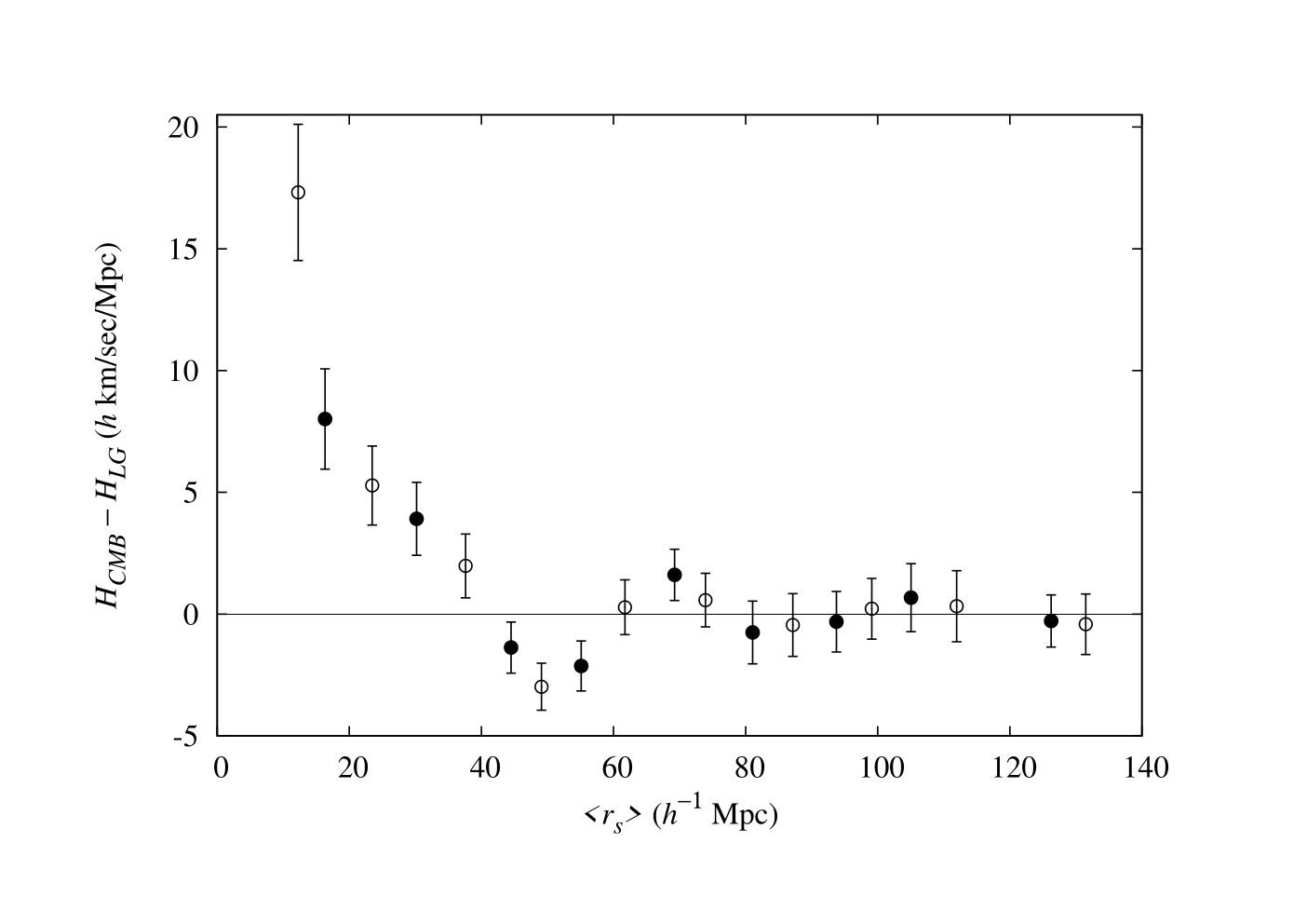
The results of our analysis are shown in Fig. 3, where we plot $\delta H_{s}$ for both the CMB and LG frames, for the two independent choices of shells given in Table 1, along with the difference $(H_{s})_{\rm CMB}-(H_{s})_{\rm LG}$. We computed the result for the LS also; it is essentially indistinguishable from the LG frame.

The values of $\delta H_{s}$ are positive, consistent with the results of LS08, and consistent with the fact that in a universe whose volume is dominated by voids a spherical average will inevitably include more voids than the denser filaments and walls if one averages on scales comparable to the diameters of the largest typical voids, leading to a higher than average $H_{s}$ as compared to the asymptotic value $\bar{H}_{\lower 2.0pt\hbox{$\scriptstyle 0$}}$.

It is clear that the variance of the spherically averaged LG or LS frame Hubble flow is less than that of the CMB frame. In both frames the Hubble flow averaged in spherical shells gives $\delta H_{s}$ within $2\sigma$ of uniform in almost all shells⁵⁵ 5 The one small exception is that $\delta H_{\lower 2.0pt\hbox{$\scriptstyle\hbox{\sevenrm CMB}$}}$ is $2.1\sigma$ from uniform for shell 9 with $100\,h^{-1}<r\leq 112.5\,h^{-1}\hbox{Mpc}$ and ${\bar{r}}_{\lower 2.0pt\hbox{$\scriptstyle 9$}}=105.0\,h^{-1}\hbox{Mpc}$. In general, the LG frame flow is still somewhat closer to uniform than the CMB frame flow in the outer regions. For all shells with ${\bar{r}}_{s}\geq 69.2\,h^{-1}\hbox{Mpc}$ the LG frame flow is within 1.36$\sigma$ of uniform. for ${\bar{r}}_{s}\geq 55.1\,h^{-1}\hbox{Mpc}$. However, particularly for values ${\bar{r}}_{s}<37.6\,h^{-1}\hbox{Mpc}$, the LG/LS frame has $\delta H_{s}$ much closer to uniform than the CMB frame, and the average LG/LS frame flow is even within 1.2$\sigma$ of uniform in the range $12.3\,h^{-1}<{\bar{r}}_{s}\leq 23.5\,h^{-1}\hbox{Mpc}$, whereas the average CMB frame flow is 4.0$\sigma$ – 7.0$\sigma$ from uniform in the same range. Since the Local Sheet itself is defined within $r<6.25\,h^{-1}\hbox{Mpc}$, this is not a result that would be readily expected with the standard interpretation of peculiar velocities.

The statistical significance of the relative uniformity of the averaged flow in the two frames can now be determined by summing the mean square differences from a uniform $\delta H=0$ expectation,

for each choice of rest frame in all shells outside an inner cutoff shell, $r_{s}$, as the inner cutoff is varied. An inner cutoff is commonly applied to eliminate the contribution of large peculiar velocities near the origin, and given the reinterpretation we follow in this paper, the effect of varying the cutoff is particularly interesting. The probability, $P_{\lower 2.0pt\hbox{$\scriptstyle\hbox{\sevenrm CMB}$}}(r_{s})$ or $P_{\lower 2.0pt\hbox{$\scriptstyle\hbox{\sevenrm LG}$}}(r_{s})$, of a uniform Hubble flow for each choice of rest frame and cutoff is then calculated directly from the complementary incomplete gamma function for the chi square distribution with the relevant number of degrees of freedom. A Bayes factor $B(r_{s})=P_{\lower 2.0pt\hbox{$\scriptstyle\hbox{\sevenrm LG}$}}/P_{\lower 2.0pt\hbox{$\scriptstyle\hbox{\sevenrm CMB}$}}$ for each choice of inner cutoff is determined for the two independent choices of shells in Table 1. The resulting values of $\ln B$ are tabulated in Table 1, and plotted as a function of $r_{s}$ in Fig. 4. We also determined $P_{\lower 2.0pt\hbox{$\scriptstyle\hbox{\sevenrm LS}$}}/P_{\lower 2.0pt\hbox{$\scriptstyle\hbox{\sevenrm CMB}$}}$ for the LS relative to the CMB; however, the values obtained gave Bayes factors which were essentially indistinguishable from those tabulated for the LG relative to the CMB.

Fig. 4 reveals a number of interesting features. The fact that overall the LG frame is more uniform is demonstrated by $\ln B$ being everywhere positive. If we consider a large inner cutoff, $r_{s}\geq 106.25\,h^{-1}\hbox{Mpc}$ then the difference in uniformity of the two frames has $\ln B\leq 1$, which is not statistically significant. With cutoffs in the range $37.5\,h^{-1}\leq r_{s}\leq 100\,h^{-1}\hbox{Mpc}$ we find $1<\ln B<3$ with positive evidence in favour of the LG frame being the more uniform. Bringing the cutoff down to $r_{s}=37.5\,h^{-1}\hbox{Mpc}$ gives $\ln B=3.6$ increasing the Bayesian evidence to strong. For cutoffs $r_{s}\leq 25\,h^{-1}\hbox{Mpc}$ the Bayesian evidence becomes very strong, $\ln B>5$. Different adjectives are used to describe the strongest Bayesian evidence [45, 46]; since $\ln B>10$ for any inner cutoff with $r_{s}<14.5\,h^{-1}\hbox{Mpc}$ Jeffreys’ terminology of “decisive evidence” in favour of the relative uniformity of the Hubble flow in the LG frame seems to be appropriate.

We must be careful, however, in the determination of statistical confidence, since there are also statistically significant departures from uniformity in the LG and LS frames also, as is consistent with the presence of foreground structures.

The nonlinear effects of the foreground structures can be seen by computing the goodness of fit probability, $Q_{s}$, given by the complementary incomplete gamma function for $\chi_{s}^{2}$ in shell $s$ with $\nu=N_{s}-1$ degrees of freedom. In Table 1 a bad linear fit is indicated in both the CMB and LG frames for shells $s\leq 4$ (unprimed) or $s\leq 3^{\prime}$ (primed) since $Q_{s}$ is less than 0.1 and equivalently the reduced $\chi^{2}$ per degree of freedom is significantly in excess of one.

We have investigated the extent to which the relative magnitude of the Bayes factor is driven by the greater scatter relative to a linear law, rather than by the difference of the linear fit of the Hubble constant from its asymptotic value. The results of this investigation are presented in Appendix A. We find that when the data points which contribute the greatest scatter relative to a linear law are excluded, leading to a high goodness of the fit, then the Bayes factors are somewhat reduced. However, the Bayesian evidence for the greater uniformity of the LG frame Hubble flow, relative to that of the CMB frame, remains very strong.

The outer shells with $s\geq 5$ (unprimed) or $s\geq 4^{\prime}$ (primed) all have a strong goodness of fit in the full data set of Table 1. This is also true in the outermost, $r>156.25\,h^{-1}\hbox{Mpc}$ shell, although it only contains 91 points. This outer shell, which is used to anchor the asymptotic value of the Hubble constant and its uncertainty, has an almost perfect goodness of fit $Q_{s}=0.999$ and a reduced $\chi^{2}$ of $0.59$ per degree of freedom in both frames.

Some hints about the nature of the effects which contribute to the deviations from a uniform linear Hubble law can be discerned by comparing $\delta H_{s}$ in the shells where the deviations from uniformity become statistically significant. Perhaps the most interesting feature is that counter to the overall trend, the individual CMB frame shells $\{4,4^{\prime},5\}$ with mean distances in the range⁶⁶ 6 Each bound is the average of the mean distances of the shell where the CMB frame is more uniform with the mean distance of the neighbouring shell where the LG frame is more uniform. $41.0\,h^{-1}\leq{\bar{r}}_{s}\leq 58.4\,h^{-1}\hbox{Mpc}$ have a closer to uniform $H_{s}$ than the corresponding LG frame shells. In the cumulative Bayes factor this adds a negative contribution, and reduces the overall $\ln B$ to $0.92$ at ${\bar{r}}_{s}=49.1\,h^{-1}\hbox{Mpc}$, even though adjacent points have $\ln B>2$.

Another important point is to consider how the nonlinear dependence of $H_{s}$ on the individual $cz_{i}$ in the regression formula (2) can lead to systematic offsets when applying boosts. Suppose we are in a frame in which the spherically averaged variance in the Hubble flow is minimized, which of course can be a frame other than the LG or LS one. Now change reference frame by applying a uniform boost to all data points, so that

where $\phi_{i}$ is the angle on the sky between the data point and the boost direction. Then $(cz_{i})^{2}\to(cz_{i}^{\prime})^{2}=cz_{i}^{2}+2cz_{i}v\cos\phi_{i}+v^{2}\cos^{2}\phi_{i}$ in the numerator of (2), and $cz_{i}r_{i}\to cz_{i}^{\prime}r_{i}=cz_{i}r_{i}+r_{i}\cos(\phi_{i})$ in the denominator.

If we perform a spherically symmetric average (2) on data which is reasonably uniformly distributed over the celestial sphere⁷⁷ 7 The absence of data in the ZoA does not affect this argument, since the gaps in the data set are symmetrically distributed on opposite sides of the sky. The argument would fail if there was a significant lack of data on one side of the sky only. then on average each positive contribution of the linear terms $v\cos\phi_{i}$ in the sums in the numerator and denominator of the boosted frame $H_{s}^{\prime}$ will be counterbalanced by a negative contribution from a $v\cos\phi_{j}$ on the opposite side of the sky. The linear contributions are therefore roughly self-canceling, leaving a dominant contribution to the difference

where $\left\langle f_{i}\right\rangle_{s}\equiv(\sum_{i=1}^{N_{s}}f_{i}\sigma_{i}^{-2})(\sum_{i=1}^{N_{s}}\sigma_{i}^{-2})^{-1}$ is a weighted average. If we now consider (8) applied to successive shells with different values of $s$, then given a uniformly symmetrical distribution of data the weighted average $\left\langle(v\cos\phi_{i})^{2}\right\rangle_{s}\mathop{\sim}\limits\frac{1}{2}v^{2}$ in the numerator will be roughly constant from shell to shell, while putting the leading order approximation $cz_{i}\simeq H_{\lower 2.0pt\hbox{$\scriptstyle 0$}}r_{i}$ in the denominator we find

Consequently, for symmetrically distributed data the effect of incorporating a boost in the redshift data is an additional contribution to the spherically averaged Hubble constant which is inversely proportional to the averaged square distance. The difference between the CMB and LG frames in Fig. 3 does indeed show hints of such a dependence. Of course, the LG frame itself may incorporate such a dependence with respect to whatever frame has the minimum variance in $H_{s}$, only to a lesser extent.

We stress that by our method of analysis the effect of a spurious boost is to add a spherically symmetric, or monopole, “Hubble bubble” type variation to the Hubble relation. This feature makes the present analysis very different to the standard peculiar velocity approach, where the focus is on dipole or higher multipole variations.

We summarize the results of this section as follows. Although there are significant foreground structures which distort the spherically averaged Hubble flow in a statistically significant manner, the LG frame has a much smaller monopole Hubble flow variance than the CMB frame, counter to standard expectations. Nonetheless, there is a particular range of distances at roughly $40\,h^{-1}\mathop{\hbox{${\lower 3.8pt\hbox{$<$}}\atop{\raise 0.2pt\hbox{$\sim$}}$}}r\mathop{\hbox{${\lower 3.8pt\hbox{$<$}}\atop{\raise 0.2pt\hbox{$\sim$}}$}}60\,h^{-1}\hbox{Mpc}$ for which the boost to the standard CMB frame produces an apparently more uniform spherically symmetric average flow. This is the first evidence for the hypothesis we will present in Sec. V, namely that rather than being a transformation which puts us in the frame in which the Hubble flow is most uniform at our own point, the boost to the CMB frame is actually compensating for the effect of foreground structures largely associated with distance scales of order $40\,h^{-1}$ to $60\,h^{-1}\hbox{Mpc}$. To better understand these structures we now consider angular averages.

We have adapted the technique of MD07 to produce a series of maps of an angular average value of $cz/r$ over the sky. At each grid point on the sky, a mean $H_{\alpha}$ is calculated in which the value of $cz_{i}/r_{i}$ for each data point is weighted according to its angular separation from the grid point, with a Gaussian window function whose standard deviation, $\sigma_{\lower 2.0pt\hbox{$\scriptstyle\theta$}}$, determines the smoothing scale. The technical details are described in Appendix B. We applied the averages (26)–(28) both without an inverse variance (IV) weighting using (22), and alternatively with an IV weighting using (30). The small differences between these two methods did not affect our conclusions.

In Fig. 5 we plot the contour maps of angular Hubble flow variance produced using the whole COMPOSITE data set in a single sphere, in both the CMB and LG rest frames. This allows a direct comparison to MD07 who considered only 76 points in a single sphere in the CMB rest frame.

To study radial variations one can simultaneously break the sample into independent shells as in Sec. II. There is enough data in the COMPOSITE sample to reliably establish a quadrupole and perhaps higher order multipoles in many of the shells of Table 1. However, our first aim is to determine the gross features of the relative angular variation. We will therefore perform the most simple of radial separations: we divide the data into an inner ($r<r_{o}$) and an outer ($r>r_{o}$) sphere, with a boundary $r_{o}$ which we vary, and reperform the Gaussian window averages.

We show a subset of the resulting sky maps in Figs. 6 and 7 for the CMB and LG rest frames, with the boundary between the inner and outer spheres taking the values $12.5\,h^{-1}$, $20\,h^{-1}$, $40\,h^{-1}$ and $60\,h^{-1}$ Mpc.

The maps are of course not entirely independent, as there is overlap of data between the outer shells for small $r_{o}$ and the inner shells of maps with larger $r_{o}$. The extent of overlap of sources, and their angular distribution, can be determined roughly from the numbers given in Table 1 and in Fig. 2, where points within individual shells are shown. Working with maps which are not independent shows how power in the dipole is transferred from the outer to inner sphere as $r_{o}$ is varied.

The first observation we make is that although both frames reveal a dipole structure, the nature of the dipole has important differences between the two frames. In the CMB frame the difference between the inner and outer spheres is not very strong. In the outer sphere the two poles migrate from being both in the northern hemisphere in the $r>12.5\,h^{-1}\hbox{Mpc}$ map to both being close to the galactic equator in the $r>60\,h^{-1}\hbox{Mpc}$ map, while the poles in the corresponding interior spheres become localized to the northern hemisphere. However, the strength of the dipole feature does not vary significantly between the inner and outer spheres, nor with the variation of the boundary $r_{o}$ between the inner and outer spheres. The fact that both poles are in the northern hemisphere in most of the CMB frame plots also means of course that the dipole is less strong than for example in the $r>12.5\,h^{-1}\hbox{Mpc}$ LG frame map, for which the poles are closer to $180^{\circ}$ apart.

By contrast to the CMB frame, in the LG frame there is a significant radial dependence to the Hubble variance dipole evident in Fig. 7. With the division set at $r_{o}=12.5\,h^{-1}\hbox{Mpc}$ there is very strong dipole feature in the outer $r>12.5\,h^{-1}\hbox{Mpc}$ sphere, which is stronger than in the full sample map of Fig. 5. By contrast, within the inner $12.5\,h^{-1}\hbox{Mpc}$ sphere any dipole signature is masked by other multipoles which appear equally as strong.

As the division scale $r_{o}$ is increased the relative power in the dipole in the inner sphere in the LG frame maps increases substantially, so that by the time we reach $r_{o}=60\,h^{-1}\hbox{Mpc}$ the inner sphere shows a dipole almost as distinct as the outer sphere of the $r_{o}=12.5\,h^{-1}\hbox{Mpc}$ map. At the same time the dipole in the outer $r>60\,h^{-1}\hbox{Mpc}$ map becomes less distinct. This is consistent with our finding in the previous section that the structures principally responsible for the Hubble flow variance lie within $r<65\,h^{-1}\hbox{Mpc}$. This conclusion will be confirmed by an independent analysis of the data in Sec. III.2 below.

We remark that the dipole feature in the LG frame can be seen by eye in the colour coded peculiar velocities relative to $H_{s}$ in each shell, as shown in Fig. 2: in shells 2 and 3, which cover the range $12.5\,h^{-1}<r<37.5\,h^{-1}\hbox{Mpc}$ there is a clear concentration of negative peculiar velocities (blue) in the upper left quadrant and positive peculiar velocities (red) in the lower right quadrant, which correlate with the dipole structure in Fig. 7. These concentrations of peculiar velocities become more and more diluted by the contributions of peculiar velocities of the opposite sign in shells 4 and 5, where $37.5\,h^{-1}<r<62.5\,h^{-1}\hbox{Mpc}$. In shells with $r>62.5\,h^{-1}\hbox{Mpc}$ the areas previously associated with the dipole feature contain similar numbers of positive and negative peculiar velocities.

The fact that the CMB frame dipole shows far less variation than the LG frame dipole as $r_{o}$ is varied is consistent with the hypothesis that it is not directly associated with the structures defining the Hubble flow variance but is rather due to an overall systematic, namely the relative boost to the CMB frame, as discussed in Sec. II.3.

The above statements are of course made from a simple inspection of the sky maps by eye. However, the statements can be quantified by performing a spectral analysis on the sky maps. To this end we digitized the contour maps into 1 square degree regions and performed a multipole analysis using HEALPIX⁸⁸ 8 http://healpix.jpl.nasa.gov/ [47] to determine the relative power in the $C_{\ell}$ coefficients. On account of the Gaussian window averaging there is aliasing at the $25^{\circ}$ scale, and information for the high multipoles is not reliable. However, since multipoles with $\ell\geq 4$ are very much suppressed a good measure of the significance of the dipole can be estimated by determining the quadrupole to dipole ratio, $C_{2}/C_{1}$, and octupole to dipole ratio, $C_{3}/C_{1}$, as listed in Table 2 in the inner and outer spheres as the boundary, $r_{o}$, is varied in the CMB, LG and LS frames. The inner and outer $C_{2}/C_{1}$ ratios are also illustrated graphically for the CMB and LG frames in Fig. 8.

In the LG frame $C_{2}/C_{1}=0.061$ in the outer $r>12.5\,h^{-1}\hbox{Mpc}$ sphere, representing a small quadrupole relative to dipole while $C_{2}/C_{1}=0.653$ in the corresponding inner sphere representing a quadrupole roughly comparable to the dipole. By contrast in the CMB frame with $r_{o}=12.5\,h^{-1}\hbox{Mpc}$, the respective ratios are $C_{2}/C_{1}=0.096$ ($0.123$) in the outer (inner) sphere, indicating a dipole which is similar in both spheres, and less clearly defined than in the outer LG frame.

In the inner sphere the ratio $C_{2}/C_{1}$ in the LG frame drops substantially for $r_{o}\geq 30\,h^{-1}\hbox{Mpc}$, and maintains a value in the range $0.09$ – $0.12$ when $40\,h^{-1}\leq r_{o}\leq 90\,h^{-1}\hbox{Mpc}$. This is of course higher than the same ratio in the outer sphere; but the inner sphere value includes in every case a contribution from the innermost shell in which the dipole and quadrupole are comparable.

The outer dipole is stronger in the LG frame than the CMB frame except for the values $40\,h^{-1}\mathop{\hbox{${\lower 3.8pt\hbox{$<$}}\atop{\raise 0.2pt\hbox{$\sim$}}$}}r\mathop{\hbox{${\lower 3.8pt\hbox{$<$}}\atop{\raise 0.2pt\hbox{$\sim$}}$}}60\,h^{-1}\hbox{Mpc}$, for which the situation is reversed. The outer CMB dipole is strongest for $r>50\,h^{-1}\hbox{Mpc}$, when the quadrupole/dipole ratio drops to a minimum $C_{2}/C_{1}=0.023$ as compared to $C_{2}/C_{1}=0.032$ in the LG frame. However, when $r_{o}\geq 70\,h^{-1}\hbox{Mpc}$ the outer CMB dipole becomes less distinct again. As we saw earlier the variance in the spherically averaged Hubble flow was less in the CMB frame in the range $35\,h^{-1}\mathop{\hbox{${\lower 3.8pt\hbox{$<$}}\atop{\raise 0.2pt\hbox{$\sim$}}$}}r\mathop{\hbox{${\lower 3.8pt\hbox{$<$}}\atop{\raise 0.2pt\hbox{$\sim$}}$}}60$ $\,h^{-1}\hbox{Mpc}$. It appears that the boost to the CMB frame is also having the effect of making the angular variance of the CMB frame Hubble flow more dipole-like over this particular radial range.

Table 2 shows that the quadrupole and higher order multipoles are at least an order of magnitude smaller than the dipole in the range $15\mathop{\hbox{${\lower 3.8pt\hbox{$<$}}\atop{\raise 0.2pt\hbox{$\sim$}}$}}r\mathop{\hbox{${\lower 3.8pt\hbox{$<$}}\atop{\raise 0.2pt\hbox{$\sim$}}$}}65\,h^{-1}\hbox{Mpc}$, and therefore a simple dipole law can be reliably used in this range. However, for $r_{o}>90\,h^{-1}\hbox{Mpc}$ the ratio $C_{2}/C_{1}$ increases substantially, so caution should be exercised about fitting a simple dipole in the outermost shells.

It is difficult to provide statistical bounds on the angular orientation and magnitude of the Hubble flow variance dipole with Gaussian window averaging. However, a completely independent analysis can be made by fitting the raw data to a simple linear dipole law

for the LG and CMB rest frames, where in each case $\phi$ is the angle on the sky between each galaxy and the direction $(\ell_{d},b_{d})$ which defines the best fit dipole axis. This method is similar to that used in Fig. 9 of Ref. [48] or Fig. 8 of Ref. [49].

In each case we determine the four parameters $H_{d}$, $\beta$, $\ell_{d}$ and $b_{d}$ by a least squares fit of $H_{d}$ and the linear parameters $\beta_{x}=\beta\cos\ell_{d}\cos b_{d}$, $\beta_{y}=\beta\cos\ell_{d}\sin b_{d}$, and $\beta_{z}=\beta\sin b_{d}$. Details are given in Appendix C. The results of the analysis for the same independent shells chosen in Table 1 are tabulated in Table 7, and the corresponding dipole amplitudes are plotted in Fig. 9. Here statistical 1$\sigma$ uncertainties are shown.

Monte Carlo simulations, discussed in Appendix D, establish that random reshuffles of the angular data in each shell are consistent with zero dipole. We also determine a probability in excess of random of the dipole law providing a better fit, and consequently a statistical confidence that the dipole in each shell is indeed non-zero.

We see from Fig. 9 that the range of radial shells over which the CMB frame provides a better fit to the monopole Hubble law than the LG frame also coincides with a dramatic difference in changes to the dipole in the two frames. The magnitudes of the dipoles in the two frames coincide in shell $3$ with ${\bar{r}}_{\lower 2.0pt\hbox{$\scriptstyle 3$}}=30.2\,h^{-1}\hbox{Mpc}$, taking the values $\beta_{\lower 2.0pt\hbox{$\scriptstyle\hbox{\sevenrm CMB}$}}=(14.0\pm 1.2)h\,\hbox{km}\,\hbox{s}^{-1}\,\hbox{Mpc}^{-1}$ and $\beta_{\lower 2.0pt\hbox{$\scriptstyle\hbox{\sevenrm LG}$}}=(14.2\pm 1.2)h\,\hbox{km}\,\hbox{s}^{-1}\,\hbox{Mpc}^{-1}$ respectively. They also coincide in shell $5^{\prime}$, with ${\bar{r}}_{\lower 2.0pt\hbox{$\scriptstyle 5^{\prime}$}}=61.7\,h^{-1}\hbox{Mpc}$, where they take the reduced values $\beta_{\lower 2.0pt\hbox{$\scriptstyle\hbox{\sevenrm CMB}$}}=(5.8\pm 1.3)h\,\hbox{km}\,\hbox{s}^{-1}\,\hbox{Mpc}^{-1}$ and $\beta_{\lower 2.0pt\hbox{$\scriptstyle\hbox{\sevenrm LG}$}}=(5.4\pm 1.2)h\,\hbox{km}\,\hbox{s}^{-1}\,\hbox{Mpc}^{-1}$. However, the dipoles exhibit very different behaviour for the shells in between. In particular, the CMB dipole magnitude reaches a minimum of $\beta=(2.6\pm 0.6)h\,\hbox{km}\,\hbox{s}^{-1}\,\hbox{Mpc}^{-1}$ (close to zero dipole) in shell 4, for which ${\bar{r}}_{\lower 2.0pt\hbox{$\scriptstyle 4$}}=44.5\,h^{-1}\hbox{Mpc}$, whereas for the LG frame $\beta=(14.9\pm 0.8)h\,\hbox{km}\,\hbox{s}^{-1}\,\hbox{Mpc}^{-1}$ in the same shell. The CMB frame dipole then increases while the LG frame dipole decreases so the two take similar values at ${\bar{r}}_{\lower 2.0pt\hbox{$\scriptstyle 5^{\prime}$}}=61.7\,h^{-1}\hbox{Mpc}$. The dipole directions in each frame are strongly consistent in shells 4 to 6 in the range $37.5\,h^{-1}\leq r\leq 62.5\,h^{-1}\hbox{Mpc}$.

The analysis of Appendix D shows that in shells 3 to 5’ our principal conclusions above concerning the relative magnitudes of the dipoles are supported to the level of at least 99.9% confidence. We therefore have a statistically robust justification for the conclusion that the boost from the LG to CMB frame is compensating for structures in the range $30\,h^{-1}\mathop{\hbox{${\lower 3.8pt\hbox{$<$}}\atop{\raise 0.2pt\hbox{$\sim$}}$}}r\mathop{\hbox{${\lower 3.8pt\hbox{$<$}}\atop{\raise 0.2pt\hbox{$\sim$}}$}}62\,h^{-1}\hbox{Mpc}$.

There are some further changes to the dipoles in the outer shells. A small residual dipole of amplitude $\mathop{\sim}\limits 5\,\hbox{km}\,\hbox{s}^{-1}\,\hbox{Mpc}^{-1}$ and roughly consistent direction is maintained in the LG frame in shells 5’ to 7, at the 90% confidence level. Beyond this scale there is no significant LG frame dipole, with the exception of shell 10. By contrast a dipole is found with at least 90% confidence level in all shells 5’ to 10 the CMB frame, and with more than 95% confidence the shells 8 and 9 which lack a significant LG frame dipole.

Although there appears to be a significant dipole in both frames in shell 10, we note from Fig. 8 that the quadrupole to dipole ratio in the Gaussian window averages begins to increase significantly at $r_{o}\mathop{\sim}\limits 100\,h^{-1}\hbox{Mpc}$. Given a strong quadrupole, and the fact that the LG dipole axis is roughly orthogonal to the largest mass concentration in shell 10 – the Shapley Concentration – we should be careful not to draw strong conclusions from the fit of a simple dipole law (10) in the outer shell, as the magnitude may change once higher multipoles are included. The COMPOSITE sample does not have enough data in shell 10 to constrain the quadrupole; considerably more data is required.

The analysis of the previous subsection provides the strongest direct evidence that there is a correlation between the structures responsible for both the monopole and dipole variations of the Hubble law in the range $30\,h^{-1}\mathop{\hbox{${\lower 3.8pt\hbox{$<$}}\atop{\raise 0.2pt\hbox{$\sim$}}$}}r\mathop{\hbox{${\lower 3.8pt\hbox{$<$}}\atop{\raise 0.2pt\hbox{$\sim$}}$}}62\,h^{-1}\hbox{Mpc}$. However, to make contact with the result of analyses in the peculiar velocity formalism, and with the Gaussian window averages, it is also useful to consider the results of a dipole law fit on all data outside (inside) a sphere $r>r_{o}$ ($r\leq r_{o}$).

The results averaged in an outer sphere are tabulated in Table 8 of Appendix C, and the corresponding dipole magnitudes are plotted in Fig. 10. In the LG frame there is a very strong dipole with magnitude $\beta=11.4\pm 0.4\,\hbox{km}\,\hbox{s}^{-1}\,\hbox{Mpc}^{-1}$ for $r_{o}=15\,h^{-1}\hbox{Mpc}$, which decreases to a typical value $\beta\mathop{\sim}\limits 3.5\,\hbox{km}\,\hbox{s}^{-1}\,\hbox{Mpc}^{-1}$ for the largest values of $r_{o}$ in Table 8, which is of order $3\sigma$ different from zero. If we consider only those cases with goodness of fit $Q>0.1$ then the most abrupt decrease in $\beta$ occurs in the range $40\,h^{-1}\leq r_{o}\leq 55\,h^{-1}\hbox{Mpc}$ where $\beta$ decreases from $6.9\pm 0.4\,\hbox{km}\,\hbox{s}^{-1}\,\hbox{Mpc}^{-1}$ to $3.5\pm 0.5\,\hbox{km}\,\hbox{s}^{-1}\,\hbox{Mpc}^{-1}$.

The diminishing of the LG frame dipole at is consistent with the results of the previous two subsections. Furthermore the angular position of the dipole for $20\,h^{-1}\mathop{\hbox{${\lower 3.8pt\hbox{$<$}}\atop{\raise 0.2pt\hbox{$\sim$}}$}}r_{o}\mathop{\hbox{${\lower 3.8pt\hbox{$<$}}\atop{\raise 0.2pt\hbox{$\sim$}}$}}45\,h^{-1}\hbox{Mpc}$ is consistently in the range $(\ell_{d},b_{d})=(83^{\circ}\pm 6^{\circ},-39^{\circ}\pm 3^{\circ})$ while the dipole is strong, but the angular position then wanders once its magnitude is reduced to residual levels. For $r_{o}\mathop{\hbox{${\lower 3.8pt\hbox{$>$}}\atop{\raise 0.2pt\hbox{$\sim$}}$}}80\,h^{-1}\hbox{Mpc}$ the typical position of the residual dipole differs from that of the inner dipole by $80^{\circ}$ – $100^{\circ}$ in galactic longitude. The direction coincides with that of the data in shell 10, which contains the only significant dipole in the outer regions.

By contrast, the magnitude of $\beta$ is initially smaller in the CMB frame for small values of $r_{o}$, with a value $\beta=6.1\pm 0.4\,\hbox{km}\,\hbox{s}^{-1}\,\hbox{Mpc}^{-1}$ at $15\,h^{-1}\hbox{Mpc}$ which decreases somewhat to $\beta=4.1\pm 0.5$ at $r_{o}=40\,h^{-1}\hbox{Mpc}$. However, $\beta$ then increases to $5.6\pm 0.6\,\hbox{km}\,\hbox{s}^{-1}\,\hbox{Mpc}^{-1}$ at $r_{o}=55\,h^{-1}\hbox{Mpc}$, and for larger $r_{o}$ its value remains roughly constant at this level, which is of order 4$\sigma$ – 7$\sigma$ different from zero. Furthermore, over the entire range $15\,h^{-1}\leq r\leq 120\,h^{-1}\hbox{Mpc}$ the direction $(\ell_{d},b_{d})$ remains within 1$\sigma$ of the “dark flow” direction $(\ell,b)=(296^{\circ},14^{\circ})\pm 13^{\circ}$ found by Kashlinsky et al. [49] for X--ray clusters in the range⁹⁹ 9 When restricted to the larger scales, $0.12\leq z\leq 0.3$, the dark flow direction is $(267^{\circ},34^{\circ})\pm 15^{\circ}$, which coincides with the direction of the residual CMB dipole in the LG frame. $0.05\leq z\leq 0.3$. It also within 1$\sigma$ of the bulk flow direction $(\ell,b)=(287^{\circ}\pm 9^{\circ},8^{\circ}\pm 6^{\circ})$ found by Watkins, Feldman and Hudson [18] for all values $20\,h^{-1}\leq r_{o}\leq 115\,h^{-1}\hbox{Mpc}$. For the largest values of $r_{o}$ in Table 8 the direction¹⁰¹⁰ 10 In the outermost shell $11$ of Table 7 with $r>156.25\,h^{-1}\hbox{Mpc}$, the uncertainty in the dipole position in the CMB frame is essentially the whole sky, meaning that there is not enough data to constrain the dipole in this range, as is confirmed by the analysis of section D. In the LG frame the magnitude of the dipole in this shell is just 1.2$\sigma$ from $\beta=0$. remains consistent with the bulk flow direction $(\ell,b)=(319^{\circ}\pm 18^{\circ},7^{\circ}\pm 14^{\circ})$ of Turnbull et al. [24]. This suggests that as far as the dipole direction is concerned the slight difference between the results of WFH09, FWH10 and Ref. [24] is accounted for by the latter study having a greater mean depth.

For the largest values of $r_{o}$ in Table 8 the CMB frame dipole direction is also consistent with some other cosmic dipoles that have been observed: a dipole in the fine structure constant [50]–[52] and the maximum temperature asymmetry [53].

A comparison of Fig. 9 and Fig. 10 shows that analysing the data only in terms of smoothed dipoles on large scales – as is implicit in the peculiar velocities approach – can hide much information. In particular, the residual LG frame smoothed dipole at $r\mathop{\hbox{${\lower 3.8pt\hbox{$>$}}\atop{\raise 0.2pt\hbox{$\sim$}}$}}80\,h^{-1}\hbox{Mpc}$ is accounted for by a feature in shell 10, whereas there is no significant LG frame dipole in shells 8 and 9. By contrast there is a CMB frame dipole in the shell by shell analysis; thus its nature is different, consistent with our hypothesis of Sec. II.3.

A large dipole structure in the Hubble flow across the sky is consistent with a foreground density gradient leading to concentrations of more rapidly expanding void regions in one sector of the sky, and less rapidly expanding wall regions in the opposite sector. A detailed understanding of the structures within $30\,h^{-1}\hbox{Mpc}$ may be gained from the work of Ref. [10], and a viewing of the associated video¹¹¹¹ 11 http://ifa.hawaii.edu/$\mathop{\sim}\limits$tully/pecv_12min_sound_qt.mov is particularly instructive. Sky maps of structures on larger scales are given by Erdoğdu et al. [54] using the 2 Micron All-Sky Redshift Survey (2MASS).

The distinctive feature of the location of our galaxy is that it is in a thin filamentary sheet, the LS, which defines the supergalactic $(X,Y)$ plane, on the edge of a Local Void of at least $30\,h^{-1}\hbox{Mpc}$ diameter. While large void regions dominate one side of the sky, wall regions dominate the other side of the sky with the superclusters of Centaurus, Hydra and Norma being particularly prominent. Our Local Sheet and nearby filamentary sheets such as the Leo Spur are of modest density. The Virgo Cluster appears to be the closest region of the thick section of a dense nearby wall; however, it lies almost in the supergalactic plane of the LS, rather than along the axis which defines the greatest density contrast between the nearby voids and walls.

In this particular situation our galaxy is neither in the middle of one of the largest typical voids of $30\,h^{-1}\hbox{Mpc}$ diameter, nor is it in the middle of one of the thick wall regions. Rather it is in the transition zone between void and modest wall structures, close to the edge of both. In this circumstance the observed dipole pattern of Hubble flow variance might be expected to be the dominant one. Since the spatial width of typical walls is generally smaller than the diameter of the largest typical voids, observers located in the middle of a thick wall region with extent in their $(X,Y)$ plane, with larger typical voids some way off and equidistant along their $\pm Z$ axes, might in contrast to our situation expect to see a more dominant quadrupole Hubble variance.

The angular extent of various structures must also be important in determining how close the pattern of Hubble flow variance is to a dipole. A pure step function contains many higher multipoles, so a simple division of the whole sky into two hemispheres of uniform faster and slower expansion would contain many higher multipoles. Since voids have a purer ellipsoidal geometry than walls, in terms of defining the relevant angular scales it is the voids which will more clearly delineate the dipole density gradient.

Some estimate of the angular scales of the nearest voids can be obtained from the work of Tully et al. [10]. However, since the distances of many galaxies in their survey are not known Tully et al. [10] present their diagrams in redshift space, which are subject to redshift space distortions as large as the Hubble flow variance that we are endeavouring to measure.

Our own Local Void comprises three separate smaller volumes: the Inner Local Void, and the Local Voids North and South, which are separated by filamentary thin wall structures [10]. Here “north” and “south” refer to directions orthogonal to the LG in supergalactic coordinates; and since the plane of our galaxy is roughly orthogonal to that of the LS, this means that supergalactic “north” and “south” indicate directions principally along the galactic longitude axis relative to the supergalactic north pole at $\ell=47.37^{\circ}$, $b=6.32^{\circ}$.

The Inner Local Void, which is ellipsoidal with its major axis roughly parallel to the Local Sheet, is the structure that covers the largest fraction of the sky in the Local Void complex. From Fig. 10 of [10] we estimate that it covers at least 40–60% of one hemisphere, given the uncertainties of redshift space distortions. In any case we expect it to be too large a fraction of the sky to give a pure dipole. This is confirmed by splitting the inner and outer shells at $r_{o}=12.5\,h^{-1}\hbox{Mpc}$, since the inner shell should just exclude the Inner Local Void while retaining the Local Voids North and South. As shown in the first panel of Fig. 7 and in Table 2, the inner sphere in these cases has similar power in the quadrupole.

The dipole axis appears to be principally defined by structures within the range $30\,h^{-1}$ – $62\,h^{-1}\hbox{Mpc}$, which lies beyond the scales explicitly identified by Tully et al. [10]. However, using the 2MASS survey Erdoğdu et al. [54] have reconstructed the density field in shells every $20\,h^{-1}\hbox{Mpc}$ out to $160\,h^{-1}\hbox{Mpc}$. To define a dipole, rather than simply locating the largest overdensity or underdensity, one must find an axis where the integrated density gradient, including foregrounds, is maximized. If we compare¹²¹² 12 Note that Ref. [54] places galactic longitude $\ell=0^{\circ}$ in the centre of their skymaps, rather than to the right edge as we do. the results of Sec. III.2 and B.1 to Fig. 3 of Ref. [54] we see that the minimum Hubble variance pole coincides with the near side of the Centaurus--Hydra Wall on one side of the sky and the maximum Hubble variance pole coincides with the Andromeda Void on the opposite side of the sky. Our axis to the Andromeda Void passes through the Inner Local Void and the edge of the Local Void North¹³¹³ 13 In the terminology of Ref. [10] the “Local Void North” comprises the region denoted “Delphinus” in Fig. 3 of Ref. [54] together with an adjacent large $\delta<0$ area extending to just above the galactic plane, $b\mathop{\sim}\limits 6$, with $47^{\circ}<\ell<90^{\circ}$. The “Local Void South” of Ref. [10] is similarly much larger than the area marked “LV” in Fig. 3 of Ref. [54] and extends to adjacent $\delta<0$ regions above the galactic plane, with $\ell<47^{\circ}$..

The centre of the Hydra Supercluster is at $r=(34.9\pm 2.5)\,h^{-1}\hbox{Mpc}$, $(\ell,b)=(269.6^{\circ},26.5^{\circ})$, and the centre of the Centaurus Supercluster is at $(31.5\pm 2.6)\,h^{-1}\hbox{Mpc}$, $(\ell,b)=(302.4^{\circ},21.6^{\circ})$. These radial distances are close to the radial scale at which the CMB frame Hubble flow begins to be more uniform than the LG one. In the next sky map plotted in Ref. [54], at $r=40\,h^{-1}\hbox{Mpc}$, the Hydra Supercluster remains very dense near the Hubble variance angular minimum while on the opposite side of the sky the Andromeda void has begun to close up, but an adjacent void complex Cygnus–Aquarius has opened up, maintaining the dipole density gradient. By Fig. 5 of Ref. [54] at $r=60\,h^{-1}\hbox{Mpc}$, on the other hand, there are now large overdensities, Pegasus and Pisces, in the angular patch that previously contained the Hubble variance maximum, while on the opposite side of the sky in Hydra underdensities have emerged. These opposing influences will now even out the density gradients along the dipole axis. We can therefore understand why the dipole diminishes beyond $r\mathop{\sim}\limits 60\,h^{-1}\hbox{Mpc}$.

As remarked above there is no significant LG frame dipole in shells 8 and 9 there is some evidence for such dipole in shell 10. Its direction, $(\ell,b)=(348^{\circ}\pm 24^{\circ},-38^{\circ}\pm 14^{\circ})$ is at $\mathop{\sim}\limits 83^{\circ}$, roughly orthogonal to the Shapley Concentration (SC), which is centred in shell 10 and extends into parts of shells 9 and 11. Thus the small LG frame dipole in shell 10 (which points from an underdense region to Abell 576) is not correlated to the SC. Indeed in the region, $300^{\circ}<\ell<330^{\circ}$, $15^{\circ}<b<45^{\circ}$, bounding the SC the numbers of positive and negative peculiar velocities with respect to the shell mean Hubble constant are equal in both shells 10 and 11, and almost equal in shell 9. The fact that the SC does not participate in a strong dipole may be due to significant mass concentrations on roughly the opposite side of the sky: see Ref. [54], Figs. 8, 9.

Since the quadrupole/dipole ratio is strong in shell 10, extra data is required to isolate the quadrupole before drawing strong conclusions about the magnitude of the dipole in this shell. However, we remark that effects on the Hubble flow at this scale might indeed be expected if the wall–to–wall distance–redshift is modified at the BAO scale: we are near one wall (defined by Virgo–Centaurus–Hydra) which is separated from more distant structures such as the SC by the $100\,h^{-1}\hbox{Mpc}$ BAO distance. Since the BAO enhancement is treated in the linear regime of perturbation theory, we might naturally expect the magnitude of nearby Hubble flow variations driven by a BAO enhancement to be significantly smaller than the “nonlinear regime” dipole amplitude observed at $r\mathop{\hbox{${\lower 3.8pt\hbox{$<$}}\atop{\raise 0.2pt\hbox{$\sim$}}$}}55\,h^{-1}\hbox{Mpc}$. This would also suggest that much high quality data in the range $100\,h^{-1}\mathop{\hbox{${\lower 3.8pt\hbox{$<$}}\atop{\raise 0.2pt\hbox{$\sim$}}$}}r\mathop{\hbox{${\lower 3.8pt\hbox{$<$}}\atop{\raise 0.2pt\hbox{$\sim$}}$}}150\,h^{-1}\hbox{Mpc}$ is needed to fully constrain any potential variations.

References

- [1] A. Kogut, C. Lineweaver, G.F. Smoot, et al., Astrophys. J. 419, 1 (1993).
- [2] D.J. Fixsen, E.S. Cheng, J.M. Gales, J.C. Mather, R.A. Shafer, and E.L. Wright, Astrophys. J. 473, 576 (1996).
- [3] D.W. Hogg, D.J. Eisenstein, M.R. Blanton, N.A. Bahcall, J. Brinkmann, J.E. Gunn, and D.P. Schneider, Astrophys. J. 624, 54 (2005).
- [4] F. Sylos Labini, N.L. Vasilyev, L. Pietronero, and Y.V. Baryshev, Europhys. Lett. 86, 49001 (2009).
- [5] M. Scrimgeour, T. Davis, C. Blake, et al., Mon. Not. R. Astr. Soc. 425, 116 (2012).
- [6] R.G. Clowes, K.A. Harris, S. Raghunathan, L.E. Campusano, I.K. Soechting, and M.J. Graham, Mon. Not. R. Astr. Soc. 429, 2910 (2013).
- [7] M.J. Hudson, R.J. Smith, J.R. Lucey, and E. Branchini, Mon. Not. R. Astr. Soc. 352, 61 (2004).
- [8] D.D. Kocevski and H. Ebeling, Astrophys. J. 645, 1043 (2006).
- [9] C.M. Springob, K.L. Masters, M.P. Haynes, R. Giovanelli, and C. Marinoni, Astrophys. J. Suppl. 172, 599 (2007).
- [10] R.B. Tully, E.J. Shaya, I.D. Karachentsev, H.M. Courtois, D.D. Kocevski, L. Rizzi, and A. Peel, Astrophys. J. 676, 184 (2008).
- [11] I.D. Karachentsev, O.G. Kashibadze, D.I. Makarov, and R.B. Tully, Mon. Not. R. Astr. Soc. 393, 1265 (2009).
- [12] G. Lavaux, R.B. Tully, R. Mohayaee, and S. Colombi, Astrophys. J. 709, 483 (2010).
- [13] I. Antoniou and L. Perivolaropoulos, J. Cosmol. Astropart. Phys. 12 (2010) 012.
- [14] J. Colin, R. Mohayaee, S. Sarkar, and A. Shafieloo, Mon. Not. R. Astr. Soc. 414, 264 (2011).
- [15] D.C. Dai, W.H. Kinney, and D. Stojkovic, J. Cosmol. Astropart. Phys. 04 (2011) 015.
- [16] A. Weyant, M. Wood-Vasey, L. Wasserman, and P. Freeman, Astrophys. J. 732, 65 (2011).
- [17] I. Iwata and P. Chamaraux, Astron. Astrophys. 531, A87 (2011).
- [18] R. Watkins, H.A. Feldman, and M.J. Hudson, Mon. Not. R. Astr. Soc. 392, 743 (2009).
- [19] H.A. Feldman, R. Watkins, and M.J. Hudson, Mon. Not. R. Astr. Soc. 407, 2328 (2010).
- [20] A. Kashlinsky, F. Atrio-Barandela, D. Kocevski, and H. Ebeling, Astrophys. J. 686, L49 (2008).
- [21] A. Kashlinsky, F. Atrio-Barandela, H. Ebeling, A. Edge, and D. Kocevski, Astrophys. J. 712, L81 (2010).
- [22] A. Nusser and M. Davis, Astrophys. J. 736, 93 (2011).
- [23] Y.Z. Ma and D. Scott, Mon. Not. R. Astr. Soc. 428, 2017 (2013).
- [24] S.J. Turnbull, M.J. Hudson, H.A. Feldman, M. Hicken, R.P. Kirshner, and R. Watkins, Mon. Not. R. Astr. Soc. 420, 447 (2012).
- [25] M.L. McClure and C.C. Dyer, New Astron. 12, 533 (2007).
- [26] N. Li and D.J. Schwarz, Phys. Rev. D 78, 083531 (2008).
- [27] D.L. Wiltshire, Class. Quantum Grav. 28, 164006 (2011).
- [28] M. Tegmark, A. de Oliveira-Costa, and A.J.S. Hamilton, Phys. Rev. D 68, 123523 (2003).
- [29] K. Land and J. Magueijo, Phys. Rev. Lett. 95, 071301 (2005).
- [30] H.K. Eriksen, A.J. Banday, K.M. Gorski, F.K. Hansen, and P.B. Lilje, Astrophys. J. 660, L81 (2007).
- [31] J. Hoftuft, H.K. Eriksen, A.J. Banday, K.M. Gorski, F.K. Hansen, and P.B. Lilje, Astrophys. J. 699, 985 (2009).
- [32] J. Kim and P. Naselsky, Astrophys. J. 714, L265 (2010).
- [33] P.A.R. Ade, et al., arXiv:1303.5083 (2013).
- [34] D.L. Wiltshire, New J. Phys. 9, 377 (2007).
- [35] D.L. Wiltshire, Phys. Rev. Lett. 99, 251101 (2007).
- [36] D.L. Wiltshire, Phys. Rev. D 78, 084032 (2008).
- [37] D.L. Wiltshire, Phys. Rev. D 80, 123512 (2009).
- [38] F. Hoyle and M.S. Vogeley, Astrophys. J. 566, 641 (2002).
- [39] F. Hoyle and M.S. Vogeley, Astrophys. J. 607, 751 (2004).
- [40] D.C. Pan, M.S. Vogeley, F. Hoyle, Y.Y. Choi, and C. Park, Mon. Not. R. Astr. Soc. 421, 926 (2012).
- [41] W.L. Freedman, B.F. Madore, B.K. Gibson, et al., Astrophys. J. 553, 47 (2001).
- [42] T.R. Lauer and M. Postman, Astrophys. J. 425, 418 (1994).
- [43] W.H. Press, B.P. Flannery, S.A. Teukolsky, and W.T. Vetterling, Numerical Recipes, (Cambridge University Press, 1986).
- [44] C.L. Bennett, M. Halpern, G. Hinshaw, et al., Astrophys. J. Suppl. 148, 1 (2003).
- [45] R.E. Kass and A.E. Raftery, J. Am. Statist. Assoc. 90, 773 (1995).
- [46] R. Trotta, Mon. Not. R. Astr. Soc. 378, 72 (2007).
- [47] K.M. Gorski, E. Hivon, A.J. Banday, B.D. Wandelt, F.K. Hansen, M. Reinecke, and M. Bartelman, Astrophys. J. 622, 759 (2005).
- [48] A. Sandage, Astrophys. J. 307, 1 (1986).
- [49] A. Kashlinsky, F. Atrio-Barandela, D. Kocevski, and H. Ebeling, Astrophys. J. 691, 1479 (2009).
- [50] J.K. Webb, J.A. King, M.T. Murphy, V.V. Flambaum, R.F. Carswell, and M.B. Bainbridge, Phys. Rev. Lett. 107, 191101 (2011).
- [51] J.A. King, J.K. Webb, M.T. Murphy, et al.Mon. Not. R. Astr. Soc. 422, 3370 (2012).
- [52] A. Mariano and L. Perivolaropoulos, Phys. Rev. D 86, 083517 (2012).
- [53] A. Mariano and L. Perivolaropoulos, Phys. Rev. D 87, 043511 (2013).
- [54] P. Erdoğdu, O. Lahav, J.P. Huchra, et al., Mon. Not. R. Astr. Soc. 373, 45 (2006).
- [55] R.B. Partridge and D.T. Wilkinson, Phys. Rev. Lett. 18, 557 (1967).
- [56] J.M. Stewart and D.W. Sciama, Nature 216, 748 (1967).
- [57] P.J.E. Peebles and D.T. Wilkinson, Phys. Rev. 174, 2168 (1968).
- [58] A. Mészáros and Z. Molnár, Astrophys. J. 470, 49 (1996).
- [59] M.J. Rees and D.W. Sciama, Nature 217, 511 (1968).
- [60] S. Jha, A.G. Riess, and R.P. Kirshner, Astrophys. J. 659, 122 (2007).
- [61] C. Gordon, K. Land, and A. Slosar, Mon. Not. R. Astr. Soc. 387, 371 (2008).
- [62] P.J.E. Peebles, Principles of Physical Cosmology, (Princeton University Press, 1993).
- [63] E.V. Linder, Phys. Rev. D 72, 043529 (2005).
- [64] M. Bilicki, M. Chodorowski, G.A. Mamon, and T. Jarrett, Astrophys. J. 741, 31 (2011).
- [65] B.M. Leith, S.C.C. Ng, and D.L. Wiltshire, Astrophys. J. 672, L91 (2008).
- [66] P.R. Smale and D.L. Wiltshire, Mon. Not. R. Astr. Soc. 413, 367 (2011).
- [67] P.R. Smale, Mon. Not. R. Astr. Soc. 418, 2779 (2011).
- [68] J.A.G. Duley, M.A. Nazer, and D.L. Wiltshire, Class. Quantum Grav. 30, 175006 (2013).
- [69] T. Buchert, Gen. Relativ. Grav. 32, 105 (2000).
- [70] T. Buchert, Gen. Relativ. Grav. 40, 467 (2008).
- [71] R. Keisler, C.L. Reichardt, K.A. Aird, et al., Astrophys. J. 743, 28 (2011).
- [72] P.A.R. Ade, et al., arXiv:1303.5076 (2013).
- [73] M. Maturi, K. Dolag, A. Waelkens, V. Springel, and T. Ensslin, Astron. Astrophys. 476, 83 (2007).
- [74] K. Bolejko, Gen. Relativ. Grav. 41, 1737 (2009).
- [75] H. Alnes and M. Amarzguioui, Phys. Rev. D 74, 103520 (2006).
- [76] J. Grande and L. Perivolaropoulos, Phys. Rev. D 84 023514, (2011).
- [77] K. Bolejko and J.S.B. Wyithe, J. Cosmol. Astropart. Phys. 02 (2009) 020.
- [78] K. Bolejko, private communication.
- [79] K. Bolejko, M.A. Nazer and D.L. Wiltshire, in preparation.
- [80] P. Szekeres, Commun. Math. Phys. 41, 55 (1975).
- [81] K. Bolejko and M.N. Célérier, Phys. Rev. D 82, 103510 (2010).
- [82] K. Bolejko, Gen. Relativ. Grav. 41, 1585 (2009).
- [83] R.A. Sussman and K. Bolejko, Class. Quantum Grav. 29, 065018 (2012).
- [84] N. Kaiser, Mon. Not. R. Astr. Soc. 227, 1 (1987).
- [85] J. Guy, P. Astier, S. Nobili, N. Regnault, and R. Pain, Astron. Astrophys. 443, 781 (2005).
- [86] J. Guy, P. Astier, S. Baumont, et al., Astron. Astrophys. 466, 11 (2007).
- [87] M. Kowalski, D. Rubin, G. Aldering, et al., Astrophys. J. 686, 749 (2008).
- [88] M. Hicken, W.M. Wood-Vasey, S. Blondin, et al., Astrophys. J. 700, 1097 (2009).
- [89] R. Amanullah, C. Lidman, D. Rubin, et al., Astrophys. J. 716, 712 (2010).
- [90] R. Kessler, A. Becker, D. Cinabro, et al., Astrophys. J. Suppl. 185, 32 (2009).
- [91] I. Zehavi, A.G. Riess, R.P. Kirshner, and A. Dekel, Astrophys. J. 503, 483 (1998).
- [92] A. Conley, R.G. Carlberg, J. Guy, D.A. Howell, S. Jha, A.G. Riess, and M. Sullivan, Astrophys. J. 664, L13 (2007).
- [93] I. Finkelman, N. Brosch, A.Y. Kniazev, et al., Mon. Not. R. Astr. Soc. 390, 969 (2008).
- [94] I. Finkelman, N. Brosch, A.Y. Kniazev, et al., Mon. Not. R. Astr. Soc. 409, 727 (2011).
- [95] A.G. Riess, L. Macri, S. Casertano, et al., Astrophys. J. 730, 119; (E) 732, 129 (2011).
- [96] W. Percival, B.A. Reid, D.J. Eisenstein, et al., Mon. Not. R. Astr. Soc. 401, 2148 (2010).
- [97] F. Beutler, C. Blake, M. Colless, et al., Mon. Not. R. Astr. Soc. 416, 3017 (2011).
- [98] C. Blake, E. Kazin, F. Beutler, et al., Mon. Not. R. Astr. Soc. 418, 1707 (2011).
- [99] H.K. Eriksen, F.K. Hansen, A.J. Banday, K.M. Gorski, and P.B. Lilje, Astrophys. J. 605, 14; (E) 609, 1198 (2004).
- [100] A. de Oliveira-Costa, M. Tegmark, M. Zaldarriaga, and A. Hamilton, Phys. Rev. D 69, 063516 (2004).
- [101] D.J. Schwarz, G.D. Starkman, D. Huterer, and C.J. Copi, Phys. Rev. Lett. 93, 221301 (2004).
- [102] C.J. Copi, D. Huterer, D.J. Schwarz, and G.D. Starkman, Mon. Not. R. Astr. Soc. 367, 79 (2006).
- [103] P.E. Freeman, C.R. Genovese, C.J. Miller, R.C. Nichol, and L. Wasserman, Astrophys. J. 638, 1 (2006).
- [104] N. Hand, G.E. Addison, E. Aubourg, et al., Phys. Rev. Lett. 109, 041101 (2012).
- [105] G. Lavaux, N. Afshordi, and M.J. Hudson, Mon. Not. R. Astr. Soc. 430 1617, (2013).
- [106] R. Keisler, Astrophys. J. 707, L42 (2009).
- [107] S.J. Osborne, D.S.Y. Mak, S.E. Church, and E. Pierpaoli, Astrophys. J. 737, 98 (2011).
- [108] F. Atrio-Barandela, A. Kashlinsky, H. Ebeling, D. Kocevski, and A. Edge, Astrophys. J. 719, 77 (2010).
- [109] F. Atrio-Barandela, A. Kashlinsky, H. Ebeling, and D. Kocevski, arXiv:1211.4345 (2012).
- [110] P.A.R. Ade, et al., arXiv:1303.5090 (2013).
- [111] F. Atrio-Barandela, Astron. Astrophys. 557, A116 (2013).
- [112] G.F.R. Ellis and J.E. Baldwin, Mon. Not. R. Astr. Soc. 206, 377 (1984).
- [113] P.A.R. Ade et al., arXiv:1303.5087 (2013).
- [114] M. Rubart and D.J. Schwarz, Astron. Astrophys. 555, A117 (2013).
- [115] C. Blake and J. Wall, Nature 416, 150 (2002).
- [116] A.K. Singal, Astrophys. J. 742, L23 (2011).
- [117] C. Gibelyou and D. Huterer, Mon. Not. R. Astr. Soc. 427, 1994 (2012).
- [118] M.A. Abramowicz, S. Bajtlik, J.P. Lasota, and A. Moudens, Acta Astronomica 57, 139 (2007).
- [119] M. Chodorowski, Mon. Not. R. Astr. Soc. 378, 239 (2007).
- [120] Grøn, Ø. and Elgarøy, Ø., Am. J. Phys. 75, 151 (2007).
- [121] M.J. Francis, L.A. Barnes, J.B. James, and G.F. Lewis, Publ. Astron. Soc. Austral. 24, 95 (2007).
- [122] G.F. Lewis, M.J. Francis, L.A. Barnes, and J.B. James, Mon. Not. R. Astr. Soc. 381, L50 (2007).
- [123] E.F. Bunn and D.W. Hogg, Am. J. Phys. 77, 688 (2009).
- [124] B.F. Roukema, Mon. Not. R. Astr. Soc. 404, 318 (2010).
- [125] V. Faraoni, Gen. Relativ. Grav. 42, 851 (2010).
- [126] P.R. Smale, PhD thesis, (Univ. of Canterbury, 2012), http://hdl.handle.net/10092/6868 .