Higher-order QCD corrections for the $W$ -boson transverse momentum distribution

Nikolaos Kidonakis^a and Richard J. Gonsalves^b

^aKennesaw State University, Physics #1202,
1000 Chastain Rd., Kennesaw, GA 30144-5591, USA

^bDepartment of Physics, University at Buffalo, The State University of New York,
Buffalo, NY 14260-1500, USA

Abstract

We present results for $W$ -boson production at large transverse momentum at LHC and Tevatron energies. We calculate complete next-to-leading-order (NLO) QCD corrections and higher-order soft-gluon corrections to the differential cross section. The soft-gluon contributions are resummed at next-to-next-to-leading-logarithm (NNLL) accuracy via the two-loop soft anomalous dimensions. Both NLO and approximate next-to-next-to-leading-order (NNLO) $p_{T}$ distributions are presented. Our numerical results are in good agreement with recent data from the LHC.

1 Introduction

The production of $W$ bosons with large transverse momentum, $p_{T}$ , has been observed and analyzed at the Tevatron over the past two decades, and significantly higher event rates have been observed as expected at the LHC over the past couple of years. This Standard Model process is a background to Higgs production and new physics and thus it is important to have accurate theoretical predictions to exploit fully the large number of events at the LHC. The $p_{T}$ distribution falls rapidly with increasing $p_{T}$ , spanning several orders of magnitude over accessible regions at hadron colliders. High- $p_{T}$ $W$ production has a clean experimental signature when the $W$ decays to leptons, and solid predictions are needed to reduce uncertainties in precision measurements of the $W$ mass and decay width. The charged leptons in complementary processes involving $Z$ bosons can be measured with somewhat higher resolution than the neutrino, but the observed event rate for $W$ bosons at the LHC is as much as a factor of ten larger than that for $Z$ bosons. Precise calculations for $W$ production at large $p_{T}$ are also needed to identify signals of possible new physics, such as new gauge bosons, which may enhance the $p_{T}$ distribution at large $p_{T}$ .

At leading order (LO) in the strong coupling $\alpha_{s}$ , a $W$ boson can be produced with large $p_{T}$ by recoiling against a single parton which decays into a jet of hadrons. The LO partonic processes for $W$ production at large $p_{T}$ are $qg\rightarrow Wq$ and $q{\bar{q}}\rightarrow Wg$ .

The NLO corrections arise from one-loop parton processes with a virtual gluon, and real radiative processes with two partons in the final state. The NLO corrections to the cross section for $W$ production at large $p_{T}$ were calculated in [1, 2] where complete analytic expressions were provided. Numerical NLO results for production at the Tevatron were also presented in Refs. [1, 2]. The predictions are consistent with the data from the CDF [3] and D0 [4] collaborations. The NLO corrections enhance the differential distributions in $p_{T}$ of the $W$ boson and they reduce the factorization and renormalization scale dependence.

Beyond NLO, it is possible to calculate contributions from the emission of soft gluons. These corrections can be formally resummed and they were first calculated to next-to-leading-logarithm (NLL) accuracy in [5]. Approximate NNLO corrections derived from the resummation were used in [6] and were shown to provide enhancements and a further reduction of the scale dependence. Numerical results were presented for the Tevatron in [6] and for the LHC at 14 TeV energy in Ref. [7]. In this paper we extend the resummation to next-to-next-to-leading-logarithm (NNLL) accuracy (see also [8]). A related study using soft-collinear effective theory (SCET) has recently appeared in [9].

In the next section we briefly review the NLO calculation and present numerical results for the $p_{T}$ distribution of the $W$ at the LHC and the Tevatron. Section 3 discusses NNLL resummation for the soft-gluon corrections. In section 4 we derive approximate NNLO expressions from the NNLL resummation and we present approximate NNLO $p_{T}$ distributions for the $W$ boson at the LHC and the Tevatron. We conclude in Section 5.

2 NLO results

We start with the leading-order contributions to $W$ production at large $p_{T}$ with a single hard parton in the final state. The two contributing sub-processes are

q(p_{a})+g(p_{b})\longrightarrow W(Q)+q(p_{c})

and

q(p_{a})+{\bar{q}}(p_{b})\longrightarrow W(Q)+g(p_{c}).

We define the kinematic variables $s=(p_{a}+p_{b})^{2}$ , $t=(p_{a}-Q)^{2}$ , $u=(p_{b}-Q)^{2}$ , and $s_{4}=s+t+u-Q^{2}$ . At the partonic threshold, where there is no available energy for additional radiation, $s_{4}\rightarrow 0$ . The partonic cross sections are singular in this limit, but the divergences are integrable when averaged over the parton distributions in the colliding hadrons.

Refer to caption — Figure 1: LO diagrams for the process $qg\rightarrow Wq$ .

The LO diagrams are shown in Figs. 1 and 2. The LO differential cross section for the $qg\rightarrow Wq$ process is

E_{Q}\frac{d\sigma^{B}_{qg\rightarrow Wq}}{d^{3}Q}=F^{B}_{qg\rightarrow Wq}\,\delta(s_{4})\,,

(2.1)

where

	$\displaystyle F^{B}_{qg\rightarrow Wq}$	$\displaystyle=$	$\displaystyle\frac{\alpha\,\alpha_{s}(\mu_{R}^{2})C_{F}}{s(N_{c}^{2}-1)}A^{qg}\,\sum_{f}\|L_{ff_{a}}\|^{2}\,,$		(2.2)
	$\displaystyle A^{qg}$	$\displaystyle=$	$\displaystyle-\left(\frac{s}{t}+\frac{t}{s}+\frac{2uQ^{2}}{st}\right)\,,$

with $\mu_{R}$ the renormalization scale, $L$ the left-handed couplings of the $W$ boson to the quark line, and $f$ the quark flavor. Also $C_{F}=(N_{c}^{2}-1)/(2N_{c})$ with $N_{c}=3$ the number of colors.

For the process $q{\bar{q}}\rightarrow Wg$ the LO result is

E_{Q}\frac{d\sigma^{B}_{q{\bar{q}}\rightarrow Wg}}{d^{3}Q}=F^{B}_{q{\bar{q}}\rightarrow Wg}\,\delta(s_{4})\,,

(2.3)

where

	$\displaystyle F^{B}_{q{\bar{q}}\rightarrow Wg}$	$\displaystyle=$	$\displaystyle\frac{\alpha\,\alpha_{s}(\mu_{R}^{2})C_{F}}{sN_{c}}A^{q\bar{q}}\,\|L_{f_{b}f_{a}}\|^{2}\,,$		(2.4)
	$\displaystyle A^{q\bar{q}}$	$\displaystyle=$	$\displaystyle\frac{u}{t}+\frac{t}{u}+\frac{2Q^{2}s}{tu}\,.$

The complete NLO corrections were derived in [1, 2]. The virtual corrections involve ultraviolet divergences which renormalize $\alpha_{s}$ and make it depend on the renormalization energy scale which we set to be ${\sim}p_{T}$ . Both the real and the virtual corrections display soft and collinear divergences which arise from the masslessness of the gluons and the zero-mass approximation for the quarks. The soft divergences cancel between real and virtual processes while the collinear singularities are factorized in a process-independent manner and absorbed into factorization-scale-dependent parton distribution functions.

The complete NLO corrections to the LO differential cross section can be written as a sum of two terms

E_{Q}\,\frac{d\hat{\sigma}^{(1)}_{f_{a}f_{b}{\rightarrow}W(Q)+X}}{d^{3}Q}=\alpha_{s}^{2}(\mu_{R}^{2})\left[\delta(s_{4})\,B(s,t,u,\mu_{R})+C(s,t,u,s_{4},\mu_{F})\right]

(2.5)

with $\mu_{F}$ the factorization scale. The coefficient functions $B$ and $C$ depend on the parton flavors. $B(s,t,u,\mu_{R})$ is the sum of virtual corrections and of singular terms ${\sim}\delta(s_{4})$ in the real radiative corrections. $C(s,t,u,s_{4},\mu_{F})$ is from real emission processes away from $s_{4}=0$ . The NLO corrections are crucial in reducing theoretical uncertainties and thus making more meaningful comparisons with experimental data for $W$ production at the Tevatron [3, 4] and the LHC [10] at large transverse momentum.

All numerical results presented in this paper are for the sum of $W^{+}$ and $W^{-}$ differential cross sections. Initial-state parton densities are taken from MSTW2008 [11]. We use the NLO central sets with the QCD coupling evolved at NLO in this section. In section 4, where we include the NNLL logarithmic corrections, we employ the NNLO central sets with the QCD coupling evolved at NNLO. The $W$ is on shell and final-state partons are integrated over the full phase space.

We begin with results for $W$ production at the LHC at center-of-mass energy $\sqrt{S}=7$ TeV and with $p_{T}$ in the range 20-500 GeV. At lower values of $p_{T}$ the fixed order NLO estimates become unreliable due to Sudakov logarithms and the comparison with experiment needs to include nonperturbative $p_{T}$ smearing. We set the factorization and renormalization scales equal to each other and denote this common scale by $\mu$ . In the left plot of Fig. 3 we plot ratios for the $W$ -boson $p_{T}$ distribution at the LHC with various choices of scale to the central result with scale $\mu=p_{T}$ . We display the scale variation of the NLO result with scale choices $p_{T}/2$ and $2p_{T}$ . We also show results for the choice of scale $\mu=\sqrt{p_{T}^{2}+m_{W}^{2}}$ but note that the numbers for this choice of scale are very similar to those for $\mu=p_{T}$ . We see that the scale variation is of the order of $\pm 10$ %. The results for these ratios are almost identical at 8 TeV energy and very similar at 14 TeV.

In the right plot of Fig. 3 we show results for $W$ production at the Tevatron at 1.96 TeV energy. Again, we display the scale variation of the NLO result with scale choices $p_{T}/2$ and $2p_{T}$ and also $\sqrt{p_{T}^{2}+m_{W}^{2}}$ . We note that the published CDF and D0 analyses [3, 4] involve older Run I data. The results presented here are also applicable to the higher luminosity and energy data from Run II.

We will say more about the scale variation in Section 4 when we include the NNLO soft-gluon corrections. Another source of uncertainty in the differential distributions comes from the parton distribution functions (PDF). We will return to the topic of PDF uncertainties when we present the approximate NNLO results in Section 4.3.

3 NNLL Resummation

Near partonic threshold the corrections from soft-gluon emissions are dominant. These corrections can be resummed to all orders using renormalization group arguments. The resummed cross section is derived in Mellin moment space, with $N$ the moment variable conjugate to $s_{4}$ , and is given formally by

	$\displaystyle{\hat{\sigma}}^{res}(N)$	$\displaystyle=$	$\displaystyle\exp\left[\sum_{i}E_{i}(N_{i})\right]\,\exp\left[E^{\prime}_{j}(N^{\prime})\right]\;\exp\left[\sum_{i}2\int_{\mu_{F}}^{\sqrt{s}}\frac{d\mu}{\mu}\;\gamma_{i/i}\left({\tilde{N}}_{i},\alpha_{s}(\mu)\right)\right]\;$		(3.1)
			$\displaystyle\hskip-56.9055pt\times\,H\left(\alpha_{s}(\sqrt{s})\right)\;S\left(\alpha_{s}\left(\frac{\sqrt{s}}{\tilde{N}^{\prime}}\right)\right)\;\exp\left[\int_{\sqrt{s}}^{{\sqrt{s}}/{\tilde{N}^{\prime}}}\frac{d\mu}{\mu}\;2\,{\rm Re}\Gamma_{S}\left(\alpha_{s}(\mu)\right)\right]$		(3.1)

where the first exponential resums the collinear and soft-gluon radiation from the inital-state partons; the second exponential resums corresponding terms from the final state; the third exponential controls the factorization scale dependence of the cross section via the parton-density anomalous dimension; $H$ is the hard-scattering function; and $S$ is the soft-gluon function describing noncollinear soft gluon emission whose evolution is controlled by the soft anomalous dimension $\Gamma_{S}$ . The first three exponentials in Eq. (3.1) are independent of the color structure of the hard scattering and thus universal [12, 13], while the functions $H$ , $S$ , and $\Gamma_{S}$ are process-specific [5, 14]. More details of the resummation formalism have been given before (see e.g. Refs. [5, 14, 15]) and will not be repeated here.

We expand the process-specific soft anomalous dimensions $\Gamma_{S}$ in the strong coupling as

\Gamma_{S}=\frac{\alpha_{s}}{\pi}\Gamma_{S}^{(1)}+\frac{\alpha_{s}^{2}}{\pi^{2}}\Gamma_{S}^{(2)}+\cdots\,.

(3.2)

The one-loop results, $\Gamma_{S}^{(1)}$ , are obtained from the ultraviolet poles in dimensional regularization of one-loop eikonal diagrams involving the colored particles in the partonic processes, Figs. 4 and 5, and were first derived in [5]. We determine the two-loop results, $\Gamma_{S}^{(2)}$ , from the ultraviolet poles of two-loop dimensionally regularized integrals for eikonal diagrams shown in Fig. 6 and related graphs involving other combinations of the eikonal lines (see also [8]).

For $qg\rightarrow Wq$ the one-loop soft anomalous dimension is

\Gamma_{S,\,qg\rightarrow Wq}^{(1)}=C_{F}\ln\left(\frac{-u}{s}\right)+\frac{C_{A}}{2}\ln\left(\frac{t}{u}\right)

(3.3)

and the two-loop soft anomalous dimension is

\Gamma_{S,\,qg\rightarrow Wq}^{(2)}=\frac{K}{2}\Gamma_{S,\,qg\rightarrow Wq}^{(1)}\,,

(3.4)

where $K=C_{A}(67/18-\zeta_{2})-5n_{f}/9$ [16] with $C_{A}=3$ and $n_{f}$ the number of light quark flavors.

For $q{\bar{q}}\rightarrow Wg$ the corresponding results are

\Gamma_{S,\,q{\bar{q}}\rightarrow Wg}^{(1)}=\frac{C_{A}}{2}\ln\left(\frac{tu}{s^{2}}\right)

(3.5)

and

\Gamma_{S,\,q{\bar{q}}\rightarrow Wg}^{(2)}=\frac{K}{2}\Gamma_{S,\,q{\bar{q}}\rightarrow Wg}^{(1)}\,.

(3.6)

We note that the proportionality of the two-loop soft anomalous dimension to the one-loop result is anticipated on general grounds from the work in Ref. [17] (see also [18, 19, 20]).

4 NNLO approximate results

By expanding the resummed cross section, Eq. (3.1), in the strong coupling we derive approximate fixed-order results. In this section we present the analytical expressions for the NNLO expansion and use them to present approximate NNLO results for the $W$ -boson transverse momentum distribution at the LHC and the Tevatron.

4.1 $qg\longrightarrow Wq$

We can write the NLO soft and virtual corrections for $qg\rightarrow Wq$ as

E_{Q}\frac{d{\hat{\sigma}}^{(1)}_{qg\rightarrow Wq}}{d^{3}Q}=F^{B}_{qg\rightarrow Wq}{\alpha_{s}(\mu_{R}^{2})\over\pi}\,\left\{c_{3}^{qg}\,\left[\frac{\ln(s_{4}/p_{T}^{2})}{s_{4}}\right]_{+}+c_{2}^{qg}\,\left[\frac{1}{s_{4}}\right]_{+}+c_{1}^{qg}\,\delta(s_{4})\right\}\,.

(4.1)

The NLO coefficients $c_{3}^{qg}$ and $c_{2}^{qg}$ of the soft-gluon terms in Eq. (4.1) can be derived from the expansion of the resummed cross section and are given by $c_{3}^{qg}=C_{F}+2C_{A}$ and

c_{2}^{qg}=-\left(C_{F}+C_{A}\right)\ln\left(\frac{\mu_{F}^{2}}{p_{T}^{2}}\right)-\frac{3}{4}C_{F}-C_{A}\ln{\left(\frac{tu}{sp_{T}^{2}}\right)}\,.

(4.2)

For later use in the NNLO results we also define the scale-independent part of $c_{2}^{qg}$ as $T_{2}^{qg}=-(3/4)C_{F}-C_{A}\ln(tu/sp_{T}^{2})$ .

The coefficient of the $\delta(s_{4})$ terms in Eq. (4.1) is given by

c_{1}^{qg}=\frac{1}{2A^{qg}}\left[B_{1}^{qg}+B_{2}^{qg}n_{f}+C_{1}^{qg}+C_{2}^{qg}n_{f}\right]+\frac{c_{3}^{qg}}{2}\ln^{2}\left(\frac{p_{T}^{2}}{Q^{2}}\right)+c_{2}^{qg}\ln\left(\frac{p_{T}^{2}}{Q^{2}}\right)\,,

(4.3)

with $B_{1}^{qg}$ , $B_{2}^{qg}$ , $C_{1}^{qg}$ , and $C_{2}^{qg}$ as given in the Appendix of the first paper in Ref. [2] but without the renormalization counterterms and using $f_{A}\equiv\ln(A/Q^{2})=0$ [note that the terms not multiplying $A^{qg}$ in Eq. (A4) for $B_{1}^{qg}$ of Ref. [2] should have the opposite sign than shown in that paper].

The NNLO expansion of the resummed cross section involves logarithms $\ln^{k}(s_{4}/p_{T}^{2})$ with $k=0,1,2,3$ . The terms with $k=1,2,3$ were already provided in Refs. [5, 6] from NLL resummation. Terms for $k=0$ were also given in Eq. (3.8) of Ref. [6] but they were incomplete. Now that we have expressions for NNLL resummation we can provide the complete result for the $k=0$ terms.

The NNLO soft-gluon corrections for $qg\rightarrow Wq$ can be written as

E_{Q}\frac{d{\hat{\sigma}}^{(2)}_{qg\rightarrow Wq}}{d^{3}Q}=F^{B}_{qg\rightarrow Wq}\frac{\alpha_{s}^{2}(\mu_{R}^{2})}{\pi^{2}}\,{\hat{\sigma^{\prime}}}^{(2)}_{qg\rightarrow Wq}

(4.4)

with

$\displaystyle{\hat{\sigma^{\prime}}}^{(2)}_{qg\rightarrow Wq}$	$\displaystyle=$	$\displaystyle\frac{1}{2}(c_{3}^{qg})^{2}\,\left[\frac{\ln^{3}(s_{4}/p_{T}^{2})}{s_{4}}\right]_{+}+\left[\frac{3}{2}c_{3}^{qg}\,c_{2}^{qg}-\frac{\beta_{0}}{4}c_{3}^{qg}+C_{F}\frac{\beta_{0}}{8}\right]\left[\frac{\ln^{2}(s_{4}/p_{T}^{2})}{s_{4}}\right]_{+}$	(4.5)
		$\displaystyle\hskip-14.22636pt{}+\left\{c_{3}^{qg}\,c_{1}^{qg}+(c_{2}^{qg})^{2}-\zeta_{2}\,(c_{3}^{qg})^{2}-\frac{\beta_{0}}{2}\,T_{2}^{qg}+\frac{\beta_{0}}{4}c_{3}^{qg}\ln\left(\frac{\mu_{R}^{2}}{p_{T}^{2}}\right)\right.$
		$\displaystyle\hskip-14.22636pt\quad\left.{}+(C_{F}+2C_{A})\frac{K}{2}-\frac{3}{16}\beta_{0}C_{F}\right\}\left[\frac{\ln(s_{4}/p_{T}^{2})}{s_{4}}\right]_{+}$
		$\displaystyle\hskip-14.22636pt{}+\left\{c_{2}^{qg}\,c_{1}^{qg}-\zeta_{2}\,c_{3}^{qg}\,c_{2}^{qg}+\zeta_{3}\,(c_{3}^{qg})^{2}+\frac{\beta_{0}}{4}\,c_{2}^{qg}\ln\left(\frac{\mu_{R}^{2}}{s}\right)-\frac{\beta_{0}}{2}C_{F}\ln^{2}\left(\frac{-u}{p_{T}^{2}}\right)\right.$
		$\displaystyle\hskip-14.22636pt\quad{}-\frac{\beta_{0}}{2}C_{A}\ln^{2}\left(\frac{-t}{p_{T}^{2}}\right)-C_{F}\,K\,\ln\left(\frac{-u}{p_{T}^{2}}\right)-C_{A}\,K\,\ln\left(\frac{-t}{p_{T}^{2}}\right)$
		$\displaystyle\hskip-14.22636pt\quad{}+(C_{F}+C_{A})\left[\frac{\beta_{0}}{8}\ln^{2}\left(\frac{\mu_{F}^{2}}{s}\right)-\frac{K}{2}\,\ln\left(\frac{\mu_{F}^{2}}{s}\right)\right]-\left(C_{F}\frac{K}{2}-\frac{3\beta_{0}C_{F}}{16}\right)\ln\left(\frac{p_{T}^{2}}{s}\right)$
		$\displaystyle\hskip-14.22636pt\quad\left.{}+\frac{3\beta_{0}}{8}C_{F}\ln^{2}\left(\frac{p_{T}^{2}}{s}\right)+2\,D_{q}^{(2)}+D_{g}^{(2)}+B_{q}^{(2)}+2\,\Gamma^{(2)}_{S\,qg\rightarrow Wq}\right\}\,\left[\frac{1}{s_{4}}\right]_{+}\,$

with $\beta_{0}=(11C_{A}-2n_{f})/3$ and where we have used the two-loop constants (cf. [21, 22])

D_{q}^{(2)}=C_{F}C_{A}\left(-\frac{101}{54}+\frac{11}{6}\zeta_{2}+\frac{7}{4}\zeta_{3}\right)+C_{F}n_{f}\left(\frac{7}{27}-\frac{\zeta_{2}}{3}\right)\,,

(4.6)

$D_{g}^{(2)}=(C_{A}/C_{F})D_{q}^{(2)}$ , and

B_{q}^{(2)}=C_{F}^{2}\left(-\frac{3}{32}+\frac{3}{4}\zeta_{2}-\frac{3}{2}\zeta_{3}\right)+C_{F}C_{A}\left(-\frac{1539}{864}-\frac{11}{12}\zeta_{2}+\frac{3}{4}\zeta_{3}\right)+n_{f}C_{F}\left(\frac{135}{432}+\frac{\zeta_{2}}{6}\right)\,.

(4.7)

Note that the difference from Eq. (3.8) of Ref. [6] is in the $[1/s_{4}]_{+}$ terms. The higher powers of the logarithms are the same. Also note that one can determine the scale-dependent $\delta(s_{4})$ terms at NNLO. These terms are also given in Ref. [6] and will not be repeated here.

4.2 $q{\bar{q}}\longrightarrow Wg$

For the process $q{\bar{q}}\rightarrow Wg$ we can write the NLO soft and virtual corrections as

\displaystyle E_{Q}\frac{d{\hat{\sigma}}^{(1)}_{q{\bar{q}}\rightarrow Wg}}{d^{3}Q}

\displaystyle=

\displaystyle{F^{B}_{q{\bar{q}}\rightarrow Wg}}{\alpha_{s}(\mu_{R}^{2})\over\pi}\,\left\{c_{3}^{q\bar{q}}\,\left[\frac{\ln(s_{4}/p_{T}^{2})}{s_{4}}\right]_{+}+c_{2}^{q\bar{q}}\,\left[\frac{1}{s_{4}}\right]_{+}+c_{1}^{q\bar{q}}\,\delta(s_{4})\right\}\,.

(4.8)

Here the NLO coefficients $c_{3}^{q{\bar{q}}}$ and $c_{2}^{q{\bar{q}}}$ of the soft-gluon terms are $c_{3}^{q\bar{q}}=4C_{F}-C_{A}$ and

c_{2}^{q\bar{q}}=-2C_{F}\ln\left(\frac{\mu_{F}^{2}}{p_{T}^{2}}\right)-\left(2C_{F}-C_{A}\right)\ln\left(\frac{tu}{sp_{T}^{2}}\right)-\frac{\beta_{0}}{4}\,.

(4.9)

For later use in the NNLO results we also define the scale-independent part of $c_{2}^{q{\bar{q}}}$ as $T_{2}^{q{\bar{q}}}=-(2C_{F}-C_{A})\ln(tu/sp_{T}^{2})-\beta_{0}/4$ .

The coefficient of the $\delta(s_{4})$ terms in Eq. (4.8) is given by

c_{1}^{q\bar{q}}=\frac{1}{2A^{q\bar{q}}}\left[B_{1}^{q\bar{q}}+C_{1}^{q\bar{q}}+(B_{2}^{q\bar{q}}+D_{aa}^{(0)})\,n_{f}\right]+\frac{c_{3}^{q\bar{q}}}{2}\ln^{2}\left(\frac{p_{T}^{2}}{Q^{2}}\right)+c_{2}^{q\bar{q}}\ln\left(\frac{p_{T}^{2}}{Q^{2}}\right)\,,

(4.10)

with $B_{1}^{q\bar{q}}$ , $B_{2}^{q\bar{q}}$ , $C_{1}^{q\bar{q}}$ , and $D_{aa}^{(0)}$ as given in the Appendix of Ref. [2] but without the renormalization counterterms and using $f_{A}=0$ .

Again, the NNLO expansion involves logarithms $\ln^{k}(s_{4}/p_{T}^{2})$ with $k=0,1,2,3$ . The terms with $k=1,2,3$ were already provided in Refs. [5, 6] from NLL resummation, but the terms given for $k=0$ in Eq. (3.19) in [6] were incomplete. With NNLL resummation we can now provide the complete result.

The NNLO soft-gluon corrections for $q{\bar{q}}\rightarrow Wg$ can be written as

E_{Q}\frac{d{\hat{\sigma}}^{(2)}_{q{\bar{q}}\rightarrow Wg}}{d^{3}Q}={F^{B}_{q{\bar{q}}\rightarrow Wg}}\frac{\alpha_{s}^{2}(\mu_{R}^{2})}{\pi^{2}}\,{\hat{\sigma^{\prime}}}^{(2)}_{q{\bar{q}}\rightarrow Wg}

(4.11)

with

$\displaystyle{\hat{\sigma^{\prime}}}^{(2)}_{q{\bar{q}}\rightarrow Wg}$	$\displaystyle=$	$\displaystyle\frac{1}{2}(c_{3}^{q\bar{q}})^{2}\,\left[\frac{\ln^{3}(s_{4}/p_{T}^{2})}{s_{4}}\right]_{+}+\left[\frac{3}{2}c_{3}^{q\bar{q}}\,c_{2}^{q\bar{q}}-\frac{\beta_{0}}{4}c_{3}^{q\bar{q}}+C_{A}\frac{\beta_{0}}{8}\right]\left[\frac{\ln^{2}(s_{4}/p_{T}^{2})}{s_{4}}\right]_{+}$	(4.12)
		$\displaystyle\hskip-14.22636pt{}+\left\{c_{3}^{q\bar{q}}\,c_{1}^{q\bar{q}}+(c_{2}^{q\bar{q}})^{2}-\zeta_{2}\,(c_{3}^{q\bar{q}})^{2}-\frac{\beta_{0}}{2}\,T_{2}^{q\bar{q}}+\frac{\beta_{0}}{4}c_{3}^{q\bar{q}}\ln\left(\frac{\mu_{R}^{2}}{p_{T}^{2}}\right)\right.$
		$\displaystyle\hskip-14.22636pt\quad\left.{}+(4C_{F}-C_{A})\frac{K}{2}-\frac{\beta_{0}^{2}}{16}\right\}\left[\frac{\ln(s_{4}/p_{T}^{2})}{s_{4}}\right]_{+}$
		$\displaystyle\hskip-14.22636pt{}+\left\{c_{2}^{q{\bar{q}}}\,c_{1}^{q{\bar{q}}}-\zeta_{2}\,c_{3}^{q{\bar{q}}}\,c_{2}^{q{\bar{q}}}+\zeta_{3}\,(c_{3}^{q{\bar{q}}})^{2}+\frac{\beta_{0}}{4}\,c_{2}^{q{\bar{q}}}\ln\left(\frac{\mu_{R}^{2}}{s}\right)-\frac{\beta_{0}}{2}C_{F}\ln^{2}\left(\frac{-u}{p_{T}^{2}}\right)\right.$
		$\displaystyle\hskip-14.22636pt\quad{}-\frac{\beta_{0}}{2}C_{F}\ln^{2}\left(\frac{-t}{p_{T}^{2}}\right)+C_{F}\left[-K\,\ln\left(\frac{tu}{p_{T}^{4}}\right)+\frac{\beta_{0}}{4}\ln^{2}\left(\frac{\mu_{F}^{2}}{s}\right)-K\,\ln\left(\frac{\mu_{F}^{2}}{s}\right)\right]$
		$\displaystyle\hskip-14.22636pt\quad{}-\left(C_{A}\frac{K}{2}-\frac{\beta_{0}^{2}}{16}\right)\ln\left(\frac{p_{T}^{2}}{s}\right)+\frac{3\beta_{0}}{8}C_{A}\ln^{2}\left(\frac{p_{T}^{2}}{s}\right)$
		$\displaystyle\hskip-14.22636pt\quad\left.{}+2\,D_{q}^{(2)}+D_{g}^{(2)}+B_{g}^{(2)}+2\,\Gamma^{(2)}_{S\,q{\bar{q}}\rightarrow Wg}\right\}\,\left[\frac{1}{s_{4}}\right]_{+}$

where

B_{g}^{(2)}=C_{A}^{2}\left(-\frac{1025}{432}-\frac{3}{4}\zeta_{3}\right)+\frac{79}{108}C_{A}\,n_{f}+C_{F}\frac{n_{f}}{8}-\frac{5}{108}n_{f}^{2}\,.

(4.13)

The scale-dependent $\delta(s_{4})$ terms at NNLO were also provided in Eq. (3.19) of [6] and we will not repeat them here.

4.3 Numerical results

We begin with results for $W$ production at the LHC at 7 TeV energy. In Fig. 7 we plot the $W$ -boson $p_{T}$ distribution, $d\sigma/dp_{T}$ . In the left plot, we compare the NLO and the approximate NNLO results at the LHC at 7 TeV energy with $\mu=p_{T}$ . We also compare our results to recent data from ATLAS [10]. It is evident that the effect of the NNLO soft-gluon corrections grows with $p_{T}$ as one would expect, since the kinematical region near partonic threshold becomes more important at higher $p_{T}$ . The inset plot shows that the ratio of the approximate NNLO to the full NLO (i.e. the $K$ factor) grows with $p_{T}$ , and the NNLO soft-gluon corrections provide nearly a 60% enhancement at $p_{T}=500$ GeV. Since the ATLAS data use acceptance cuts and are normalized by the total fiducial cross section, we have to correct for these factors to extrapolate the experimental results for direct comparison to our $p_{T}$ distribution. We use the procedure described in [23]. We multiply the normalized ATLAS results by the total fiducial cross section and divide by the acceptances. It is clear from the comparison that the data are in very good agreement with our NNLO approximate result, which provides a better description than NLO alone. The ATLAS data only go up to a $p_{T}$ of 300 GeV and it will be interesting to see data from the LHC at even higher $p_{T}$ .

In the right plot of Fig. 7 we show ratios of the approximate NNLO result with the variation of the result with scale $\mu=p_{T}/2$ and $2p_{T}$ relative to $\mu=p_{T}$ . We also show the ratio with $\mu=\sqrt{p_{T}^{2}+m_{W}^{2}}$ and note that the results for this choice of scale are very similar to those for $\mu=p_{T}$ . Also, comparing the left plot of Fig. 3 with the right plot of Fig. 7 it is seen that the scale dependence at approximate NNLO is smaller than at NLO at intermediate values of $p_{T}$ , but it grows larger at very high $p_{T}$ values where the overall soft-gluon contribution is also larger.

We note that results for 7 TeV LHC energy have also been provided in Ref. [9] at NNLL in the SCET formalism. It is not possible to do an analytical comparison with [9] because no analytical results are provided there. It is also important to note that NNLL means different things in different approaches and also if one uses different variables within the same approach. This has been clearly explained in the context of top quark production in the review paper of Ref. [24] and applies here as well. Therefore our NNLL Mellin-space resummation is not equivalent to the NNLL SCET resummation of [9]. Related studies for top quark cross sections show that different formalisms can give very different numerical results [24].

Furthermore, it is difficult to make a meaningful numerical comparison because most of the figures in [9] plot results versus parameters that are only defined within the SCET formalism. Non-graphical results are provided in Table 1 of [9], which provides absolute integrated cross section estimates for $p_{T}>200$ GeV. The LO and NLO fixed-order results are of course in agreement with ours, but exponentiated logarithmic corrections will obviously diverge in this bin, thus making the comparison not very meaningful. At a purely numerical level, however, we note that our approximate NNLO integrated cross section at 7 TeV LHC energy above a $p_{T}$ of 200 GeV is about 20% larger than that provided in Table 1 of Ref. [9].

Finally it is important to note that here we use an NNLO expansion of the resummed expression to obtain numerical results, in order to avoid prescriptions needed to invert from moment space to momentum space. Even within a given formalism such as SCET or Mellin moments, there is a numerical difference between using NNLO expansions and attempting a full resummation (again see [24] and references therein for more details). However, this difference is typically smaller than the differences between different formalisms or prescriptions, so this is usually a point of relatively minor significance. For example both the values and uncertainties in [9] are very similar for the resummed and NNLO approximate results.

We continue with the presentation of our numerical results for the $W$ -boson $p_{T}$ distribution at the LHC. In Fig. 8 we show results for the LHC at 8 TeV energy. Although the overall $p_{T}$ distribution is enhanced at 8 TeV relative to 7 TeV, the result for the ratio of approximate NNLO over NLO shown in the inset plot is very similar (almost identical) to that at 7 TeV. Also the scale dependence at 8 TeV is almost the same as at 7 TeV as can be seen by comparing the right plots of Figs. 7 and 8.

In Fig. 9 we show the corresponding results for the LHC at 14 TeV energy. Again, the increase due to the NNLO soft-gluon corrections is more prominent at very high $p_{T}$ , reaching 90% enhancement at $p_{T}=1000$ GeV. The scale variation at the LHC at 14 TeV energy is shown on the right plot. At the very highest $p_{T}$ the scale uncertainty is significant.

Finally, we present results for the Tevatron. The left plot of Fig. 10 shows the NLO and NNLO approximate $p_{T}$ distributions at the Tevatron at $\mu=p_{T}$ , with the inset plot displaying the $K$ factor. The right plot of Fig. 10 shows the results for scale variation at the Tevatron, where there is a reduction of scale dependence at NNLO relative to that at NLO in the $p_{T}$ range shown, as can be seen by comparing the right plots of Figs. 3 and 10.

In addition to the scale variation shown in the previous figures, one can also attempt an independent variation of the factorization and renormalization scales; however, this does not affect the range of the overall uncertainty significantly, if at all.

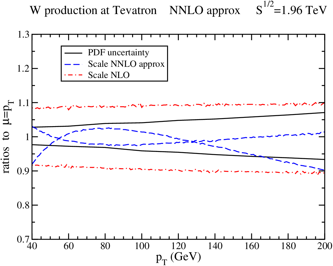
As already mentioned in Section 2, in addition to scale dependence another important source of uncertainty comes from the PDF. Here we use the PDF sets and procedure provided by MSTW2008 [11] to calculate the PDF uncertainties for $W$ production. In the left plot of Fig. 11 we compare the PDF uncertainty with the scale uncertainty at NNLO and also at NLO at the Tevatron. The scale ratios are for $\mu=p_{T}/2$ and $2p_{T}$ and are the same as already shown in the plots of the previous Tevatron figures, but displaying them together and with the PDF ratios makes the comparison of all the uncertainties easier. We note that for the Tevatron the PDF uncertainties are smaller than the NLO scale variation, but they are larger than the scale variation at approximate NNLO for most $p_{T}$ values. As mentioned earlier, the NNLO scale variation is consistently smaller than that at NLO.

In the right plot of Fig. 11 we compare the PDF uncertainty with the scale uncertainty at NNLO and also at NLO at the LHC at 8 TeV energy (the results at 7 TeV are practically the same). Here the situation is somewhat different from the Tevatron in that the upper range of the PDF uncertainty is larger than both NLO and NNLO scale variation, but the lower range is smaller than both for most $p_{T}$ values. Also the scale variation at approximate NNLO is smaller than that at NLO for moderate $p_{T}$ values but becomes larger, particularly at the lower end, at very high $p_{T}$ .

The growing NNLO contribution relative to NLO with increasing $p_{T}$ at both Tevatron and LHC energies does not appear to be an artifact of perturbation theory. The extended $p_{T}$ range made accessible by the LHC brings into play a high multiplicity of hard jets in various inclusive cross sections, and this is expected to affect the convergence of perturbative predictions. The recent ATLAS data [10] and its agreement with our theoretical results confirms this expectation. An analysis of the $Z$ distribution is underway and will be reported elsewhere.

5 Conclusions

The transverse momentum distribution of the $W$ boson receives large QCD corrections. Complete NLO calculations have been used in this paper to provide numerical results at LHC and Tevatron energies. In addition, NNLL resummation of soft-gluon corrections has been derived using two-loop soft anomalous dimensions. Approximate NNLO analytical expressions have been derived from the resummed cross section and employed to produce numerical results. The NNLO soft-gluon corrections reduce the NLO scale dependence at low and intermediate $p_{T}$ where the bulk of the data is located. In the very high $p_{T}$ region at LHC energies the soft logarithms seem to become sensitive to scale. It is possible that including hard NNLO corrections will improve this situation. The experimental bins at large $p_{T}$ are larger because the number of expected events and the $p_{T}$ resolution both decrease dramatically. Recent ATLAS data [10] are in good agreement with our numerical results. The higher-order results presented in this paper strengthen theoretical predictions for $W$ production at hadron colliders and may prove significant for new physics searches in the tail of the $p_{T}$ spectrum.

Acknowledgements

The work of N.K. was supported by the National Science Foundation under Grant No. PHY 0855421.

References

[1] P.B. Arnold and M.H. Reno, Nucl. Phys. B 319, 37 (1989); (E) B 330, 284 (1990).
[2] R.J. Gonsalves, J. Pawłowski, and C.-F. Wai, Phys. Rev. D 40, 2245 (1989); Phys. Lett. B 252, 663 (1990).
[3] CDF Collaboration, F. Abe et al., Phys. Rev. Lett. 66, 2951 (1991).
[4] D0 Collaboration, B. Abbott et al., Phys. Rev. Lett. 80, 5498 (1998) [hep-ex/9803003]; V.M. Abazov et al., Phys. Lett. B 513, 292 (2001) [hep-ex/0010026].
[5] N. Kidonakis and V. Del Duca, Phys. Lett. B 480, 87 (2000) [hep-ph/9911460].
[6] N. Kidonakis and A. Sabio Vera, JHEP 02, 027 (2004) [hep-ph/0311266].
[7] R.J. Gonsalves, N. Kidonakis, and A. Sabio Vera, Phys. Rev. Lett. 95, 222001 (2005) [hep-ph/0507317].
[8] N. Kidonakis and R.J. Gonsalves, in DPF 2011, arXiv:1109.2817 [hep-ph].
[9] T. Becher, C. Lorentzen, and M.D. Schwartz, Phys. Rev. Lett. 108, 012001 (2012) [arXiv:1106.4310 [hep-ph]].
[10] ATLAS Collaboration, G. Aad et al., Phys. Rev. D 85, 012005 (2012) [arXiv:1108.6308 [hep-ex]].
[11] A.D. Martin, W.J. Stirling, R.S. Thorne, and G. Watt, Eur. Phys. J. C 63, 189 (2009) [arXiv:0901.0002 [hep-ph]].
[12] G. Sterman, Nucl. Phys. B 281, 310 (1987).
[13] S. Catani and L. Trentadue, Nucl. Phys. B 327, 323 (1989).
[14] N. Kidonakis, in DIS 2011, arXiv:1105.4267 [hep-ph]; in DPF 2011, arXiv:1109.1578 [hep-ph].
[15] N. Kidonakis, Phys. Rev. D 81, 054028 (2010) [arXiv:1001.5034 [hep-ph]]; Phys. Rev. D 82, 054018 (2010) [arXiv:1005.4451 [hep-ph]]; Phys.Rev. D 83, 091503 (2011) [arXiv:1103.2792 [hep-ph]].
[16] K J. Kodaira and L. Trentadue, Phys. Lett. 112B, 66 (1982).
[17] S.M. Aybat, L.J. Dixon, and G. Sterman, Phys. Rev. Lett. 97, 072001 (2006) [hep-ph/0606254]; Phys. Rev. D 74, 074004 (2006) [hep-ph/0607309].
[18] L.J. Dixon, L. Magnea, and G. Sterman, JHEP 08, 022 (2008) [arXiv:0805.3515 [hep-ph]].
[19] T. Becher and M. Neubert, Phys. Rev. Lett. 102, 162001 (2009) [arXiv:0901.0722 [hep-ph]]; JHEP 06, 081 (2009) [arXiv:0903.1126 [hep-ph]].
[20] E. Gardi and L. Magnea, JHEP 03, 079 (2009) [arXiv:0901.1091 [hep-ph]]; Nuovo Cim. C 32, 137 (2009) [arXiv:0908.3273 [hep-ph]].
[21] H. Contopanagos, E. Laenen, and G. Sterman, Nucl. Phys. B 484, 303 (1997) [hep-ph/9604313].
[22] S. Moch, J.A.M. Vermaseren, and A. Vogt, Nucl. Phys. B 646, 181 (2002) [hep-ph/0209100].
[23] T. Becher, C. Lorentzen, and M.D. Schwartz, Phys. Rev. D 86, 054026 (2012) [arXiv:1206.6115 [hep-ph]].
[24] N. Kidonakis and B.D. Pecjak, Eur. Phys. J. C 72, 2084 (2012) [arXiv:1108.6063 [hep-ph]].

Higher-order QCD corrections for the WW-boson transverse momentum distribution

Abstract

1 Introduction

2 NLO results

3 NNLL Resummation

4 NNLO approximate results

4.1 q​g⟶W​qqg\longrightarrow Wq

4.2 q​q¯⟶W​gq{\bar{q}}\longrightarrow Wg

4.3 Numerical results

5 Conclusions

Acknowledgements

References

Higher-order QCD corrections for the $W$ -boson transverse momentum distribution

4.1 $qg\longrightarrow Wq$

4.2 $q{\bar{q}}\longrightarrow Wg$