clumpy: a code for -ray signals from dark matter structures
Abstract
We present the first public code for semi-analytical calculation of the -ray flux astrophysical -factor from dark matter annihilation/decay in the Galaxy, including dark matter substructures. The core of the code is the calculation of the line of sight integral of the dark matter density squared (for annihilations) or density (for decaying dark matter). The code can be used in three modes: i) to draw skymaps from the Galactic smooth component and/or the substructure contributions, ii) to calculate the flux from a specific halo (that is not the Galactic halo, e.g. dwarf spheroidal galaxies) or iii) to perform simple statistical operations from a list of allowed DM profiles for a given object. Extragalactic contributions and other tracers of DM annihilation (e.g. positrons, antiprotons) will be included in a second release.
Keywords:
Cosmic rays , Cosmology , Dark Matter , Indirect detection , Gamma-raysPROGRAM SUMMARY
Program Title: CLUMPY
Programming language: C/C++
Computer: PC and Mac
Operating system: UNIX(Linux), MacOS X
RAM: depends on the requested size of skymaps (40 Mb for a map)
Keywords: dark matter, indirect detection, gamma-rays
Classification: 1.1, 1.9
External routines/libraries: CERN ROOT11
1
http://root.cern.ch,
Doxygen22
2
http://www.doxygen.org (optional)
Nature of problem: Calculation of -ray signal from dark matter annihilation (resp. decay).
This involves a particle physics term and an astrophysical one. The focus here is on the latter.
Solution method: Integration of the DM density squared (resp. density) along a line of sight.
The code is optimised to deal with the DM density peaks
encountered along the line of sight (DM substructures).
A semi-analytical approach (calibrated on N-body simulations) is used for the
spatial and mass distributions of the dark matter substructures in the Galaxy.
Restrictions:
Some generic dark matter annihilation spectra are provided but are not included in the calculation so far as it is assumed
that the particle physics is independent of the astrophysics of the problem.
Running time: this is highly dependent of the DM profiles considered, the requested precision and integration angle :
- 1.
about 60 mn for a map towards the Galactic centre, with , NFW dark matter profiles and ;
- 2.
about 2h for the same set-up towards the anti-centre;
- 3.
0.1 to 10 DM models per second, depending on integration angle and DM profile.
1 Introduction
Despite the several astrophysical evidences pointing at the existence of dark matter (flat rotation curves of galaxies, gravitational lensing, “bullet cluster", etc.), its nature still evades us. This search has become one of the major topic in both particle physics and astrophysics and is tackled using either direct or indirect detection methods. For the former, the hope is to directly witness the interaction of a dark matter particle with a detector. The indirect approaches aim at measuring the end products of dark matter annihilation/decay (e.g., -rays, positrons, anti-protons). The detection of -rays was soon recognised to be a promising channel [1, 2]. If such a signal is yet to be measured by the existing -rays observatories (FERMI, HESS, MAGIC, VERITAS), the prospect may significantly improve with the forthcoming next-generation instruments, such as CTA [3].
Having a modelling tool that can compute the expected -ray flux from dark matter annihilation/decay in a wide range of astrophysical configurations and making it available to the community should prove very useful. This is the motivation for developing the code presented in this paper. This paper highlights clumpy’s main features but a more thorough description can be found in the documentation coming with the source code. The paper is organised as follows. Section 2 presents the formulation of the generic -ray signal calculation that is performed by clumpy, with special emphasis on the contribution from DM clumps. The code is described in sect. 3, which presents the structure, parameters and functions that are at the core of clumpy. Section 4 deals with two examples of the science that can be performed with clumpy. We conclude and discuss the future developments of the code in sect. 5.
2 Calculating the -ray flux from dark matter annihilation/decay
The -ray flux from dark matter annihilating/decaying particles is expressed as the product of a particle physics term by an astrophysical contribution. For a given experiment with a spatial resolution corresponding to an integration solid angle , at energy and pointing in the direction , the flux is written as:
| (1) |
2.1 Annihilation and decay: general statements
2.1.1 Annihilation: the particle physics term
It can be generically expressed as
| (2) |
where is the mass of the DM particle, is the annihilation cross section, the annihilation rate averaged over the DM velocity distribution, is the branching ratio into the final state and is the photon yield per annihilation. A widely accepted value for estimated from present day thermal relic density is cm3s-1 [4]33 3 Note that a velocity dependent cross section should be included in a future release of the code in order to account for the Sommerfeld effect in the calculation. This effect results in much larger cross sections for some resonant neutralino masses and therefore boost the signal for these DM candidates.. The photon spectrum is dependent on the annihilation channels. We restrict ourselves to the popular Minimal Supersymmetric Standard Model (MSSM). In this framework, the neutralino is the lightest stable supersymmetric particle and is the favoured DM candidate.
Neutralino annihilation can produce -rays in three ways: i) DM annihilates directly into two photons or , giving rise to monochromatic lines, ii) or it can annihilate into primary products, the hadronization and decay of which produce a -ray continuum, iii) finally, if charged particles are produced, internal bremsstrahlung (IB) can also contribute to the continuum. The lines are very model-dependent and given the uncertainties on the particle physics models, we did not include any in clumpy. The user is however free to implement their own function if need be. There exists in the literature several parametrisations for the -ray continuum and we have implemented that of Bergström et al. [4], and Tasitsiomi and Olinto [5]. The IB contributions is also very model dependent, and we provide one benchmark model from Bringmann et al. [6]. We refer the reader to §3.3.7 (spectra.h) for more details on these spectra.
2.1.2 Annihilation: the astrophysical contribution
The -rays being produced from the annihilation of pairs of dark matter particles, the -ray flux is proportional to the DM density squared. The second term of Eq. (1), termed astrophysical contribution, corresponds to the integration of the density squared along the line of sight (), in the observational cone of solid angle (see A and geometry.h for definitions and the geometry used)
| (3) |
where is the local DM density at distance from Earth in the direction (longitude and latitude in Galactic coordinates).
This integral is the core of the clumpy code and can be rather complicated to evaluate. The difficulty comes partially from the steepness of some DM profiles considered but also, and mainly, from the existence of DM clumps, the contribution of which must be added to the smooth Galactic DM background. Both components are dealt with hereafter.
2.1.3 Decaying dark matter
-rays can also be produced from the decay of DM. Formally, the flux is still given by Eq. (1) but the astrophysical and particle physics terms take different forms:
- 1.
The particle physics term now corresponds to the decay spectrum and no parametrisation of that term has been included in the code so far. The parametrisation from Bertone et al. [7] could be used.
- 2.
Because we are now considering a decay reaction, the astrophysics term is the integration of the density (rather that density squared as in Eq. (3)) along the line of sight, namely
(4) This quantity can be straightforwardly computed in CLUMPY by setting the flag parameter gDM_IS_ANNIHIL_OR_DECAY to false (see table 3).
2.2 Dark matter distribution
To date, there is no consensus to what the Galactic DM profile, , should be. There is some dynamical evidence that the Galactic DM halo might be triaxial [8] and numerical simulations, such as the Aquarius [9] or the Via Lactea runs [10] also find non-spherical halos. When included, the baryons tend however to make the halos more spherical [11]. In this first version of clumpy we simplify the problem (as often done) using spherically symmetric DM halos, but allowing for tri-axiality is being considered for future releases. The total averaged density profiles of the DM halos measured in these simulations are generally fitted by a form of the Zhao profile [12] :
| (5) |
where , and are respectively the inner, transition and outer slope of the profile, and a scale density and radius. The Navarro et al. [13], Moore et al. [14], and Diemand et al. [15] profiles fall in this category. Some other profiles having a log-varying inner slope [16, 17] are also included in clumpy. The reader is referred to §3.3.4 (profiles.h) for a detailed description.
Some of these DM profiles are steep enough in the inner regions to lead to a singularity of the -ray luminosity at the centre of the halo. However, a cut-off radius naturally appears, within which the DM density saturates due to the balance between the annihilation rate and the gravitational infalling rate of DM particles. The saturation density reads [18]
| (6) |
Plugged in any profile parametrisation, this saturation density defines the cut-off radius below which the annihilation rate is constant. This is a very crude description, but this is not important as this cut-off matters only for the steepest profiles () which are disfavoured by current numerical simulations.
The hierarchical scenario of galaxy formation in a -CDM cosmology is characterised by a high degree of clumpiness of the DM distribution (supported by N-body simulations) so that the total averaged density computed from these simulations corresponds to
| (7) |
where is the “true” smooth component and represents the average density from the substructures. These two components are discussed below.
2.2.1 The clumps
Whether substructures in subhalos are scaled-down versions of substructure in main halos remains an open question [9]. In this release of clumpy, we only consider one level of substructure within the halo under scrutiny (Galactic halo or individual halo such as a dwarf spheroidal galaxy), and the properties of these sub-halos can be independently chosen from that of the parent halo (see below).
Clump individual properties
In the code, all clumps have the same inner DM distribution, which can be any of the profiles discussed in §3.3.4. The mass of the clump generally suffices to determine all its properties, i.e., its size , and once an inner density profile is chosen, its scale radius and scale density . This is done using the so-called concentration parameter . Parametrisations of the mass-concentration relation have been established from numerical simulations for isolated field halos [19, 20] but the concentration generally presents a significant scatter [21]. These relations have been implemented in the code, regardless of that scatter or of the environment and formation history of the halos that can also affect the value of the concentration. We refer the reader to §3.3.6 (clumps.h) and the Doxygen documentation for more details.
Spatial and mass distribution of the clumps
Following Lavalle et al. [22], spherical symmetry is assumed and the two distributions are assumed independent44 4 Keep in mind that such an assumption fails near the Galactic centre, where small clumps are expected to be disrupted by tidal forces. In this direction, the signal from the smooth contribution dominates anyway.. If is the total number of clumps in a DM host halo, then the overall distribution of clumps is written as:
| (8) |
where the spatial and mass distribution are probabilities, respectively normalised as:
| (9) |
Analysis of N-body simulations have shown the mass distribution to vary as a simple power law
| (10) |
Given the mass and spatial distribution, the total number of clumps can be determined in two ways. If the mass fraction of clumps and the mass of the host halo are known,
with the average mass of one clump. An other approach is to know the number of clumps in a given mass interval and to calculate the total number of clumps as
Clumpy uses the first approach when dealing with substructures in individual host halos (that are not the Milky Way) and the second one for the Galactic halo clumps (numerical simulations have found about 100 clumps with masses above M⊙ in Milky Way-like halos). clumpy allows to select any of the profiles given in §3.3.4 (profiles.h) for the clump spatial distribution, independently of the choice made for the total density profile.
2.2.2 The smooth component
From the spatial distribution one can define the average clump density used in Eq. (7) as:
| (11) |
For a given total density profile and clump spatial distribution, Eq. (7) then gives the smooth density profile as
| (12) |
Using this approach, rather than providing independently a smooth and a clump profile, ensures (by construction) that the total density profiles follows the one measured in N-body simulations. This has been discussed in Pieri et al. [23].
2.3 Calculating the annihilation J-factor
The astrophysical contribution to the annihilation flux is formally given by Eq. (3). The J-factor is more explicitly written as:
| (13) |
where is given by Eq. (12) and the second term corresponds to the sum of the inner densities squared of all clumps contained with the volume element. The latter should not be confused with . Three terms arise from this equation:
| (14) |
| (15) |
and the cross product
| (16) |
2.4 Statistical considerations
Taking as a canonical value for the slope of the mass distribution, with 100 clumps above M⊙ as determined from N-body simulations, and a minimal theoretical mass of M⊙ for the smallest ones, the total number of clumps in the Milky Way halo (i.e., for ) is estimated to be , which is computationally prohibitive. Even if we are interested in a skymap only (i.e., ), the number of clumps is . This is too large a number to realise a statistical drawing according to the distribution and then numerically integrate the component for each of these clumps. However, their high number means that a statistical average can be safely performed, as long as the variance is small. The clumpy code computes the -ray flux from DM clumps by either randomly drawing clumps given user-defined spatial and mass distributions and inner DM profiles, or by calculating the mean contribution whenever the variance of this contribution is smaller than some user-defined value.
2.4.1 Averaged quantities from the continuum limit
Given the clump mass and spatial distributions given above, it is possible to define average values for the primary random variables of the problem (a clump mass and position) and the one deriving from them. The mean mass and the mean luminosity are respectively defined by
| (17) |
| (18) |
where is the intrinsic luminosity of a clump given by
| (19) |
The average of the distance to any power is written as
| (20) |
Combining these, it can be shown that the average contribution from the clumps is expressed as
| (21) |
In the same spirit, in the continuum limit the cross-product becomes
| (22) |
The importance of the cross product can easily be identified when considering that the clump spatial distribution follows the total average density profile. In that case, and , leading directly to . For a typical clump mass fraction , this cross product amounts to of the reference J-factor . This shows that when an averaged clump description is used to integrate the signal along the line of sight, this cross product is not negligible and should be taken into account. In B, it is however shown that on an individual basis, the cross product of one clump in an underlying smooth Galactic component can be safely discarded. This will apply to the clumps that need to be statistical drawn in our model (see below).
2.4.2 Variance of the clump contribution
Along a given line of sight and for a given integration angle , the average flux between and given by Eq. (21) can also be expressed as
| (23) |
where is the average number of clumps in this volume (given the distance interval and mass range considered), and the average flux of one clump (see also [24]). Using the point-like approximation, a clump of mass at a distance has a flux
| (24) |
so that, recalling that the mass of the clump and its location are independent variables,
| (25) |
The variance on the flux of a single clump is then defined as
| (26) |
The variance of a population of clumps follows as
| (27) |
2.4.3 Criterion for using the averaged description
For a given integration domain, there is a threshold mass above which the clumps are not numerous enough to be described by an averaged description. Conversely, for a given mass decade there is a critical distance below which the averaged description fails and where clumps should be statistically drawn.
The averaged description can be safely used, as long as the relative error made on the clump flux with respect to the total flux (i.e. including the smooth contribution)
| (28) |
is smaller than some user-defined prescription.
Critical distance for the clumps in the Galaxy
The RE is plotted in Fig. 1 as a function of the lower limit of the integration . As can be seen, for any required precision (e.g., 5% in Fig. 1, tagged by the dotted green line), one can infer the corresponding distance below which the relative error becomes larger than the request.

In practise, it is convenient to perform the calculation in terms of mass decades: for each decade, we find (by dichotomy) the critical distance below which clumps must be drawn55 5 This mass decade corresponds to a typical clump radius and we also check that the point-like hypothesis used to derived the continuum limit is appropriate ().. A lower limit of kpc is set on to avoid divergences for a clump sitting at the observer’s location. An example for the final number of clumps to draw below is provided in Tab. 1.
| Mass decade | # clumps | (kpc) | # clumps | # to draw |
|---|---|---|---|---|
| (Galaxy) | kpc | () | () | |
| 0 | ||||
| 0 | ||||
| 0 | ||||
| 0 | ||||
| 0 | ||||
| 3 | ||||
| 45 | ||||
| 117 | ||||
| 99 | ||||
| 44 | ||||
| 7 | ||||
| 1 | ||||
| 0 | ||||
| 0 | ||||
| 0 | ||||
| 0 |
The flowchart given in Fig. 2 summarises the various steps implemented in clumpy to obtain the skymap (see, e.g., Fig. 3).

| Name | Type | long. | lat. | d | z | prof. | ||||||
|---|---|---|---|---|---|---|---|---|---|---|---|---|
| - | - | deg | deg | kpc | - | kpc | kpc-3 | kpc | - | - | - | - |
Threshold mass for the sub-clumps in an “far-away” halo
The second case where the criterion is used is for the sub-clumps in a halo located away from us, e.g., a dSph galaxy. In that case, the distance to the clumps is known as they are all distributed within their parent halo’s radius and we can determine in a similar fashion the threshold mass above which clumps must be drawn.
3 Description of the code
Clumpy is written in C/C++ and relies of the CERN ROOT library that is publicly available from http://root.cern.ch. The main features of the code are described hereafter along with brief descriptions of its most important functions. The code’s structure is standard, with separate directories for the various pieces of code: declarations are in include/*.h, sources in src/*.cc, compiled libraries, objects and executables are respectively in the lib/, obj/, and bin/ directories.
3.1 Code executables
The code has one executable that can take three main options depending whether the user i) is interested in performing a generic analysis on the Galactic halo, ii) is focusing on a list of specific halos (e.g. dSph galaxies), or iii) wishes to perform a statistical analysis on a single object. These main three usages of the code all accommodate several cases, the details of which are given below.
3.1.1 Galactic mode: ./bin/clumpy -g[option]
This calculates the -factor for the Galactic halo, including both the smooth and the clump component. For the clump component, the mean flux or a stochastic realisation can be chosen. Note that a list of specific halos can be added to the calculation. Several options allow to select the quantity to be calculated/plotted from a text interface. A mandatory input is the parameter file clumpy_params.txt described in §3.2 and table 3. The options are the following:
- 1.
’option = -g1’ plots the total, smooth and averaged clump density in 1D, given the user-defined total density and the number of clumps in a given mass range.
- 2.
- 3.
’option = -g3’ is the same as ’-g2’ but as a function of the angular distance to the Galactic centre, for a given integration angle.
- 4.
’option = -g4’ is the same as ’-g3’ but including a list of specific objects, such as dSph galaxies.
- 5.
’option = -g5’ plots a 2D skymap of the -factor, using the averaged clump description. where
- 6.
’option = -g6’ is similar ’-g5’, but adds specific halos to the plots (e.g. dSph), to identify their contrast to the background.
- 7.
’option = -g7’ and -g8 are respectively the same as ’-g5’ and ’-g6’ but with the clumps randomly drawn from their user-defined mass and spatial distributions.
3.1.2 Halo list mode: ./bin/clumpy -h[option]
This usage of clumpy performs operations that are basically the identical to those performed in the ’Galactic’ mode (see §3.1.1), but for a list of halos that are not the Galactic halo. This mode was initially implemented for the study of dwarf spheroidal galaxies [25], but can be extended to any DM halo (e.g., galaxy clusters). If only the smooth total density profile is considered, the halo profiles are read from a simple ASCII list of profiles along with their parameters, as exemplified in Tab. 2. If sub-clumps are considered, the clumpy parameter file clumpy_params.txt must also be provided (see table 3).
Again, further options are accessed for this mode by means of a simple text-user interface:
- 1.
’-h1’ to ’-h3’ are identical to ’-g1’ to ’-g3’ but transposed to any halo that is not the Galactic DM halo;
- 2.
’-h4’ to ’-h5’ create 2D skymaps of the halo under scrutiny using respectively an averaged description or a statistical realisation for the sub-clumps within this halo;
| Name | Definition |
|---|---|
| gCOSMO_RHO0_C | Critical density of the universe [ kpc-3] |
| gCOSMO_OMEGA0_M | Present-day pressure-less matter density |
| gCOSMO_OMEGA0_LAMBDA | Present-day dark energy density |
| gDM_GAMMARAY_FLAG_SPECTRUM | -ray spectrum flag [gENUM_GAMMASPECT] |
| gDM_MMIN_SUBS | Min. mass of a DM (sub-)clump [] |
| gDM_MMAXFACTOR_SUBS | Defines max. mass of clump in host halo as |
| gDM_RHOSAT | Saturation density [ kpc-3] |
| gTYPE_CLUMPS_FLAG_CVIRMVIR† | Clump concentration flag in the parent TYPE halo[gENUM_CVIRMVIR] |
| gTYPE_CLUMPS_FLAG_PROFILE | Clump inner profile flag [gENUM_PROFILE] |
| gTYPE_CLUMPS_SHAPE_PARAMS[0-2] | Shape parameters for sub-clumps inner profile |
| gTYPE_DPDM_SLOPE | Slope subclump mass function |
| gTYPE_DPDV_FLAG_PROFILE | Spatial distribution subclumps [gENUM_PROFILE] |
| gTYPE_DPDV_RSCALE | Scale radius for the subclump distribution in the parent halo [kpc] |
| gTYPE_DPDV_SHAPE_PARAMS[0-2] | Shape parameters for the clump spatial distribution |
| gTYPE_SUBS_MASSFRACTION | Mass fraction of the parent halo in sub-clumps |
| gGAL_CLUMPS_FLAG_CVIRMVIR | Concentration flag [gENUM_CVIRMVIR] |
| gGAL_CLUMPS_FLAG_PROFILE | Clump inner profile flag [gENUM_PROFILE] |
| gGAL_CLUMPS_SHAPE_PARAMS[0-2] | Shape parameter for the Galactic clumps inner profile |
| gGAL_DPDM_SLOPE | Slope the clump mass function |
| gGAL_DPDV_FLAG_PROFILE | Clump number distribution flag |
| gGAL_DPDV_RS | Scale radius for clumps [kpc] |
| gGAL_DPDV_SHAPE_PARAMS[0-2] | Three shape parameters for the Galactic clump spatial distribution |
| gGAL_SUBS_M1 | Reference mass for gGAL_SUBS_N_INM1M2 [] |
| gGAL_SUBS_M2 | Reference mass for gGAL_SUBS_N_INM1M2 [] |
| gGAL_SUBS_N_INM1M2 | # of clumps in |
| gGAL_RHOSOL | Local DM density [GeV cm-3] |
| gGAL_RSOL | Distance Sun – Galactic centre [kpc] |
| gGAL_RVIR | Virial radius of the Galaxy [kpc] |
| gGAL_TOT_FLAG_PROFILE | Total DM profile of the Milky Way [gENUM_PROFILE] |
| gGAL_TOT_RSCALE | Scale radius for DM halo of the Milky Way [kpc] |
| gGAL_TOT_SHAPE_PARAMS[0-2] | Shape parameter for the Galactic total density profile |
| gSIMU_ALPHAINT_DEG | Integration angle [deg] |
| gSIMU_EPS | Default precision for numerical integrations |
| gSIMU_IS_ANNIHIL_OR_DECAY | For annihilating or decaying DM |
| gSIMU_SEED | Seed of random number generator |
† TYPE corresponds to the type of halo under scrutiny (not the Galactic halo): DSPH, GALAXY
or CLUSTER are the values
allowed by gENUM_TYPEHALOES in this version.
3.1.3 ’Statistical’ mode: ./bin/clumpy -s[option]
Confidence levels on the astrophysical factor , for e.g. dSphs, can also be estimated from an ASCII statistical file. The format for the latter is quite similar to the halo list file (see documentation) as it requires the profile parameters, but it differs in the sense that for a single halo, thousands of profiles ’selected’ by a statistical analysis must be provided (their respective value is necessary, although not used for all CL calculations). Such a statistical analysis can be the Markov Chain Monte Carlo (MCMC), as discussed in Charbonnier et al. [25]; Walker et al. [26]. The most important options in the statistical mode are:
- 1.
’-s2’ plots the probability density functions (PDF) and correlations of the parameters given in the statistical file;
- 2.
’-s4’ locates the confidence intervals on the PDF of each parameters;
- 3.
’-s5’ computes, for each radius from the dSph centre, the median and confidence levels of the DM density ;
- 4.
’-s6’ is the same as ’-s5’ but for , i.e. as a function of the integration angle;
- 5.
’-s7’ is same as ’-s5’ but for , i.e. as a function of the angle to the centre of the halo.
3.2 User-defined parameters
For most of the options used above, a user-define parameter file is read. Table 3 gives the list of the main parameters. Each parameter is a single word formatted as g (for global parameter) + physics keyword + parameter name. For instance, COSMO refers to cosmology-related parameters, TYPE defines the type of halo under scrutiny (dSPh galaxy, galaxy or galaxy clusters) and GAL refers to the Milky Way halo parameters. Note also that the parameters ending in FLAG_CVIRMVIR, FLAG_SPECTRUM, and FLAG_PROFILE should take values from the following enumerations:
- 1.
enum gENUM_CVIRMVIR {kB01, kENS01, kJS00} for the clump concentration;
- 2.
enum gENUM_GAMMASPECT {kSUSY_BUB98, kSUSY_TO02, kSUSY_BBE08} for the -ray spectrum;
- 3.
enum gENUM_PROFILE {kZHAO, kEINASTO, kEINASTO_N} for the DM spatial distributions (smooth and clumpy components). The corresponding shape parameters (e.g. () for kZHAO, for kEINASTO and for kEINASTO_N) should be provided by the user in the input parameter file (see below).
This enumerations allow the user to use their explicit denomination kXXX, rather than the corresponding integer number. These parameters are gathered in the ASCII file clumpy_params.txt which is formatted as “Parameter name”, “Units”, “Value”. The function load_parameters(file_name) defined in params.h reads in the input file and assigns the appropriate values to the parameters. The user can change any ‘‘Value" in this file77 7 Some of these parameters are optional and used only for specific modes[options].
3.3 clumpy libraries
The functions of clumpy are located in eleven “library” files, accordingly to their field of action. We briefly describe hereafter the most important functions of these libraries. We are omitting in this document the more minor functions, the description of which can be found in the documentation provided with the code. Also, we do not detail here what arguments are passed in these functions as it can be easily retrieved from the documentation.
3.3.1 integr.h
This library contains standard integration algorithms. The Simpson integrator with doubling step is the most widely used throughout the code to ensure that the user-defined precision is reached. Depending on the function to integrate, either linear or logarithmic stepping can be used.
3.3.2 geometry.h
In geometry.h are gathered functions performing geometrical tasks (change of coordinates, etc.). They are not essential for the presentation of the code and generally self-explanatory. We refer the reader to the extensive Doxygen documentation and to A for more details.
3.3.3 inlines.h and misc.h
These contain some definitions (unit conversion and inline functions) and miscellaneous formatting functions respectively.
3.3.4 profiles.h
This library contains all the density profiles available in the code and operations on those. Among the functions in the “profiles” section of the code, some act in a very straightforward way (e.g. squaring the density) and are not included in the present document. The reader is, once again, referred to the Doxygen documentation for a full description.
- 1.
rho_ZHAO returns the DM density of a user-defined profile having the generic functional form given in Zhao [12]
(29) The isothermal, Navarro et al. [13], Moore et al. [14], and Diemand et al. [15] profiles are all from the Zhao family. They are defined using Eq. (29) with the set of parameters of table 4. The user is required to specify these parameters in the ASCII input file.
- 2.
rho_EINASTO and rho_EINASTO_N: it has been argued that a profile with a logarithmic inner slope gives a better fit to the simulated data. This so-called Einasto is generically written as
In Navarro et al. [16] and Springel et al. [9] the Einasto profile is defined as
(30) where is the radius at which the profile’s slope , and the corresponding density. Both Navarro et al. [16] and Springel et al. [9] find to be a good fit to the smooth component of simulated halos. Springel et al. [9] further notes that allows a good description of the spatial distribution of sub-structures .
Merritt et al. [17] use an Einasto profile, slightly different from the above and given by
(31) where and . The scale radius in this relation correspond to the radius within which half of the halo mass is enclosed.
- 3.
The normalisation density of all these profiles (, or ) can be done by i) either requesting a given value for the density at a given point or ii) by requesting a given mass within a given radius. The functions set_par0_given_rhoref and set_par0_given_mref achieve the normalisation using both approaches.
- 4.
rho simply returns the value of the density by calling any of the functions above, depending on the value of the profile flag given in clumpy_params.txt.
- 5.
3.3.5 integr_los.h
This is the core of the clumpy code as it contains the routines performing the integration along the line of sight direction () and over the chosen angular resolution . Given a function where ( are spherical coordinates in the direction (see Fig. 6), the integration along the observation cone, from to is generically written as:
| (32) |
- 1.
integrand_l: returns the value of the function . A switch is included to integrate different functions of the density profile . Note that here can refer to any profile or distribution, be it the density or the spatial distribution of clumps depending on the normalisation used. The functions that can be integrated along the line of sight are:
- (a)
when calculating the clumps averaged contribution of Eq. (21).
- (b)
in order to evaluate J such as in Eq. (14).
- (c)
is used to calculate the mass fraction or number fraction of clumps in the integration volume;
- (d)
is needed when estimating the mean distance of the clumps as in Eq. (20).
- (e)
is needed when estimating the variance of distance of the clumps.
- (f)
must be evaluated to evaluate the variance on J as in Eq. (26).
Note that if decaying rather than annihilating DM is being considered, i.e. gDM_IS_ANNIHIL_OR_DECAY is false instead of true, any is replaced by in the above functions88 8 This makes some of these functions redundant for decay, but they are still required for annihilation..
A variation of this function, called integrand_lrel, is used whenever the steepness of the profile requires it (see Doxygen documentation for more details).
- (a)
- 2.
fn_beta_alpha: computes the third integrand in Eq. (32), namely the integration over . The functions to integrate roughly behave as power laws, with a varying slope, and log-step Simpson integration schemes are used (see integr.h). Some profiles can be very steep and several tests and tricks are needed to ensure the numerical stability/optimisation of the integration. The reader is again referred to the documentation for an explicit description of the integration strategy.
- 3.
fn_beta: computes the integration over the angle in Eq. (32). A simple linear Simpson integration scheme is used.
- 4.
los_integral: it is the final part of the triple integration, i.e. the integration over the angle . This is again performed quite easily with a linear Simpson scheme. This function is called whenever a single density profile is to be dealt with.
- 5.
los_integral_mix: as seen previously, it may be necessary to integrate a difference or a product of two densities along the line of sight. A flag parameter switch_rho is introduced to tell rho_mix to return either (switch_rho = 0) or (switch_rho = 1) (see profiles.h). This function then behaves identically to los_integral and uses the same flags with respect to the quantity to integrate.
3.3.6 clumps.h
All the functions related to the clumps mass and spatial distributions are gathered in this file. Here, we only give an overview of the most important ones.
- 1.
add_halo_in_map: when using the code to generate a skymap where clumps are randomly drawn from their mass and spatial distribution, this adds the J contribution of the drawn clump to the appropriate pixels. The clump is only added to a pixel if where is the pixel containing the centre of the clump and is the requested integration precision gSIMU_EPS. This avoids the clump from being integrated “too far” which would only be time consuming without changing the result.
- 2.
dpdv_XXX and set_normprob_dpdv: the former function returns the spatial distribution of the clumps as described in §2.2.1 and the second calculates the appropriate normalisation to make it a probability according to Eq. (9). The function dpdv_XXX is written in several versions depending of the reference frame and coordinate system in which the clumps are drawn (cartesian XXX=xyz, spherical centred on the galactic centre XXX=rthetapsi, spherical centred on Earth XXX=lthetapsi, or centred on Earth, in the cone , in the direction XXX=lalphabeta).
- 3.
dpdm and set_normprob_dpdm: this is the equivalent of the above but for the mass distribution of the clumps as given by Eq. (10).
- 4.
frac_nsubs_in_foi returns the number fraction of clumps in a given field of integration w.r.t. the total number of clumps in the host halo
- 5.
frac_nsubs_in_m1m2 returns the fraction of clumps with a mass in the range , given the total number of clumps.
- 6.
jcrossprod_continuum returns the value of the cross-product integrated along the l.o.s as defined by Eq. (22). This is a simple call to los_integral_mix.
- 7.
jcrossprod_interpolation interpolates the value of in the pixels of a skymap, provided that has previously been estimated in some locations of the map. This makes use of ROOT interpolation function based on Delaunay’s triangles and allows to speed-up the calculation significantly when the skymap has a (too) large number of pixels.
- 8.
j_smooth returns the -factor when a single density profile is used (e.g. ). This is a simple call to los_integral.
- 9.
j_smooth_mix is the same as above but deals with a combination of densities, e.g. when computing Eq. (14) where . This is a simple call to los_integral_mix.
- 10.
j_sub_continuum computes and returns the averaged generated by the sub-clumps in a halo, in a given line of sight.
- 11.
lum_singlehalo returns the total intrinsic luminosity of a DM halo, given its inner density profile as in Eq. (19).
- 12.
mass_singlehalo returns the total mass of a DM halo, given its inner density profile.
3.3.7 spectra.h
This library contains the different parametrisations of the average -ray spectra,
| (33) |
in the particle physics term of Eq. (2). As mentioned in §2.1.1, we have included the Bergström et al.[4] and Tasitsiomi & Olinto [5] parametrisations for the -ray continuum and the Bringmann et al. [6] expression of the internal bremsstrahlung. Defining , the three parametrisations are given by their corresponding functions below.
- 1.
dNdE_BERGSTROM returns
- 2.
dNdE_TASITSIOMI computes the -ray spectrum as
- 3.
dNdE_BRINGMANN estimates the internal bremsstrahlung contribution with
where is the fine structure constant and is the ratio of the mass of the boson to the neutralino mass .


3.3.8 stat.h
The functions included in this library perform simple statistical operations on the random variables of the problem (mass and distance of the clumps) and on quantities deriving from them (luminosity, J-factor). Ultimately, these are mainly used to determine the critical distance (or threshold mass) below (above) which clumps need to be drawn (see §2.4.3 for the adopted procedure). Given these dark matter spatial () and mass () distributions defined in §2.2.1):
- 1.
for a given mass and/or distance range, mean1cl_mass, mean1cl, mean1cl_lum2, mean1cl_l, and mean1cl_j return respectively the average mass, luminosity, luminosity squared, distance and J-factor of one clump;
- 2.
var1cl_mass, var1cl_lum, var1cl_l, and var1cl_j returns the variance of the corresponding random variable;
- 3.
finally, knowing the variance of the J-factor of one clump, find_lcrit_los and find_mthresh_los find the critical distance and threshold mass for drawing the clumps. They both rely on a simple dichotomy to bracket the desired quantity, as illustrated on Fig.1.
3.3.9 janalysis.h
This is the top-level library. It contains the main functions called when invoking any of the three options of clumpy (galactic halo, halo list or statistics, see §3.1). Note that the first word ’xxx’ of the function’s name refers to which option they belong to (xxx=gal, xxx=halo, or xxx=stat).
- 1.
xxx_j1D handles all the 1D calculations of the Galactic or halo options. It computes , , and , where is the angle measured w.r.t. the Galactic centre.
- 2.
xxx_j2D generates the 2D skymaps for the smooth, averaged and statistically drawn clump contributions. It also include the cross product term and It applies to both the Galactic and halo options.
- 3.
xxx_load_list loads the list of halo under scrutiny either for the halo mode or the statistical option. The list should be provided as an ASCII file with the format given in table 2.
- 4.
xxx_set_par* are a set of functions filling the parameters arrays to be passed to the above functions with the proper quantities (e.g., profile flag and shape parameters, concentration flag, etc.). It applies to the Galactic and halo options.
- 5.
stat_CLs is the most important function in the statistics option and computes the confidence levels of a quantity (density, J-factor) from its PDF.


4 Run examples
This section provides a few plots obtained by using the clumpy executable. Many more examples and illustrations are provided along with the Doxygen documentation.
4.1 Sky maps
Figure 3 shows two examples of a skymap of the J-factor (option ’-g7’ of clumpy_gal), when looking off the Galactic centre (left) or towards the anti-centre (right). The angular resolution is and the Galactic smooth DM density, clump distribution and clump inner profile are all assumed to follow an NFW parametrisation.
Similarly, skymaps of individual objects can be performed (option ’-h5’ of clumpy_dsph). In Fig. 4, a "generic” dwarf galaxy, including a population of subclumps, is integrated over (left), (middle), and (right). As the resolution increases, more substructures become apparent but the J-factor is strongly reduced.
4.2 dSphs and statistical tools
The three panels in Fig 5 illustrate clumpy capabilities on the dSphs. The top left and bottom figures are taken from Charbonnier et al. [25], and the top right one is a direct result of the analysis performed in the above paper. Running clumpy on the default parameters will not give these plots, but similar ones in spirit.




5 Conclusions
The clumpy code is optimised to calculate the line-of-sight integration of the density and/or the density square of the DM distributions (smooth and clump distributions). It can be used by (i) experimentalists looking for realistic -ray skymaps to calculate their new instrument sensitivity, or simply to use them in model/template analyses for the DM diffuse emission near the Galactic centre (or for dSphs), (ii) for astrophysicists working on the reconstruction of the DM content of dSphs who wish to calculate the J factor as a by-product of their study, (iii) theoreticians who want to plug their preferred particle physics model and see what is the corresponding -ray flux in the Galaxy/dSph. The code is fully documented and provides many functions that makes it versatile and flexible.
Many improvements are possible for a future release. The simplest and more straightforward ones to consider are:
- 1.
Extra-galactic signal from the local structures (e.g. local clusters, Nezri et al. in prep.), but also from the high-redshift isotropic contribution.
- 2.
The possibility to have the so-called Sommerfeld-like enhancements. This requires to couple the calculation of the spatial density of DM to the position-dependant velocity of the DM particles.
- 3.
Neutrino annihilation spectra and fluxes.
Some other improvements are intrinsically more difficult to add, as they depend on astrophysical inputs that are not well determined. Indeed, in the absence of a smoking gun signature for indirect detection (e.g. a line detection), multi-wavelength and multi-messenger analyses seem to be a compulsory approach. To do so, one needs to take into account
- 1.
the anti-proton and anti-deuteron signal;
- 2.
electron and positron production;
- 3.
secondary multi-wavelength emissions from leptons.
Finally, the clumpy code could be coupled to some particle physics code to get more specific annihilation spectra (e.g., darkSUSY, Gondolo et al. [27]; MicrOMEGAs, Belanger et al. [28]), or to some cosmic-ray propagation code (e.g. GALPROP99 9 http://galprop.stanford.edu/, DRAGON1010 10 http://www.desy.de/ maccione/DRAGON/ or USINE, Maurin et al., in preparation) to compare with the Galactic astrophysical backgrounds. This will be considered for a second release of the code.
Acknowledgements
We thank E. Nezri and J.-C. Lambert for their useful comments on the code. We also thank the anonymous referee the many constructive comments that improved both the code and the paper.
Appendix A Geometry and change of coordinates
We define two frames of reference: one attached to the observer the origin of which is the Earth, and the other linked to the Galactic Centre (see Fig. 6). The frame related to the Earth is spherical, and is identified to the Galactic coordinate system. is the distance to the Earth, the Galactic longitude is measured in the plane of the Galaxy using an axis pointing from the Earth to the Galactic Centre, the Galactic latitude is measured from the plane of the Galaxy to the object.
The Galactic Centre frame is a cartesian frame, where the and axes are in the Galactic plane, and the axis is pointing to the North Galactic pole. In this frame, the position of the Earth is , where is the distance between the Earth and the Galactic Centre.
The change of coordinates formulae are given in the documentation (geometry.h).
Appendix B Cross-product of individual clumps
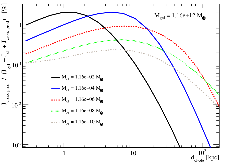
In §2.3 it has been shown that the cross-product between the underlying smooth DM density and that of all the clumps in the line of sight (when using an average description) can significantly contribute to the value of J in the line of sight. It is interesting to check what contribution it brings when considering one clump only (rather that the entire distribution). We use the same equations as in §2.3 but written for one clump only and numerically integrates J. Two configurations are explored: i) a clump embedded in the Galactic halo (fig. 7, top panels) and ii) a clump embedded in a host halo located away from the sun (fig. 7, bottom panels).
In fig. 7, the relative error made when neglecting the cross-product is plotted against i) the distance to the clump for the first configuration (top), ii) the distance of the clump to the centre of its host halo (bottom). In both cases, these curves show that, as far as one individual clump is concerned, the cross-product is completely negligible, whatever situation occurs: it amounts at most to .
References
- [1] Gunn, J. E., Lee, B. W., Lerche, I., Schramm, D. N., and Steigman, G., ApJ, 223 (1978) 1015.
- [2] Stecker, F. W., ApJ, 223 (1978) 1032.
- [3] CTA Consortium, arXiv:1008.3703, 2011.
- [4] Bergström, L., Ullio, P., and Buckley, J. H., Astroparticle Physics, 9 (1998) 137.
- [5] Tasitsiomi, A. and Olinto, A. V., Phys. Rev. D, 66 (2002) 083006.
- [6] Bringmann, T., Bergström, L., and Edsjö, J., Journal of High Energy Physics, 1 (2008) 49.
- [7] Bertone, G., Buchmüller, W., Covi, L., and Ibarra, A., J. Cosmology Astropart. Phys., 11 (2007) 3.
- [8] Law, D. R., Majewski, S. R., and Johnston, K. V., ApJ, 703 (2009) L67.
- [9] Springel, V. et al., MNRAS, 391 (2008) 1685.
- [10] Diemand, J. et al., Nature, 454 (2008) 735.
- [11] Kazantzidis, S. et al., ApJ, 611 (2004) L73.
- [12] Zhao, H., MNRAS, 278 (1996) 488.
- [13] Navarro, J. F., Frenk, C. S., and White, S. D. M., ApJ, 490 (1997) 493.
- [14] Moore, B., Governato, F., Quinn, T., Stadel, J., and Lake, G., ApJ, 499 (1998) L5.
- [15] Diemand, J., Moore, B., and Stadel, J., MNRAS, 353 (2004) 624.
- [16] Navarro, J. F. et al., MNRAS, 349 (2004) 1039.
- [17] Merritt, D., Graham, A. W., Moore, B., Diemand, J., and Terzić, B., AJ, 132 (2006) 2685.
- [18] Berezinsky, V. S., Gurevich, A. V., and Zybin, K. P., Physics Letters B, 294 (1992) 221.
- [19] Bullock, J. S. et al., MNRAS, 321 (2001) 559.
- [20] Eke, V. R., Navarro, J. F., and Steinmetz, M., ApJ, 554 (2001) 114.
- [21] Wechsler, R. H., Bullock, J. S., Primack, J. R., Kravtsov, A. V., and Dekel, A., ApJ, 568 (2002) 52.
- [22] Lavalle, J., Yuan, Q., Maurin, D., and Bi, X., A&A, 479 (2008) 427.
- [23] Pieri, L., Lavalle, J., Bertone, G., and Branchini, E., Phys. Rev. D, 83 (2011) 023518.
- [24] Lavalle, J., Pochon, J., Salati, P., and Taillet, R., A&A, 462 (2007) 827.
- [25] Charbonnier, A. et al., MNRAS 418 (2011) 1526.
- [26] Walker, M. G., Combet, C., Hinton, J. A., Maurin, D., and Wilkinson, M. I., ApJ, 733 (2011) L46.
- [27] Gondolo, P. et al., J. Cosmology Astropart. Phys., 7 (2004) 8.
- [28] Belanger, G. et al., Comput. Phys. Commun. 182 (2011) 842.