Completeness of classical $\phi^{4}$ theory on 2D lattices

The definition of CV stabilizer states starts with generalization of the Pauli group to the continuous setting [29, 30, 31, 32, 33]. For one qumode, (a term which replaces qubit in the continuous setting) the resulting group is called Heisenberg-Weyl group $W$, whose algebra of generators is spanned by the coordinate and momentum operators satisfying $[\widehat{Q},\widehat{P}]=iI$. Thus modulo $U(1)$ phases, the group $W$ is the group of unitary operators of the form $w(t,s)=e^{it\widehat{Q}+is\widehat{P}}$. Since the two unitary operators

$$\hat{X}(s)=e^{-is\widehat{P}}~~~~~~~and~~~~~~~\hat{Z}(t)=e^{it\widehat{Q}},$$

(6)

have the simple relation

$$\hat{Z}(t)\hat{X}(s)=e^{ist}\hat{X}(s)\hat{Z}(t),$$

(7)

multiplication of any two elements of $W$ can be recast in the form $X(t)Z(s)$ modulo a phase. The Heisenbergy-Weyl group can be represented on the Hilbert space of one particle, spanned by the basis states $|y\rangle_{q}$ (eigenstates of $\widehat{Q})$ or $|y\rangle_{p}$ (eigenstates of $\widehat{P}$). On these states, the operators $X$ and $Z$ act as follows:

	$\displaystyle\hat{Z}(t)|y\rangle_{q}=e^{ity}|y\rangle_{q},\hskip 28.45274pt\hat{X}(s)|y\rangle_{p}=e^{-isy}|y\rangle_{p},$		(8)
	$\displaystyle\hat{Z}(t)|y\rangle_{p}=|y+t\rangle_{p},\hskip 28.45274pt\hat{X}(s)|y\rangle_{q}=|y+s\rangle_{q}.$		(9)

Remark: Hereafter we denote the states $|y\rangle_{q}$ simply as $|y\rangle$ and use $|y\rangle_{p}$ for eigenstates of $\widehat{P}$ as above.
The CV Hadamard operator is a unitary non-Hermitian operator defined as

$$\hat{H}:=\int|y\rangle_{p}\langle y|_{q}dy\equiv\frac{1}{\sqrt{2\pi}}\int e^{ixy}|x\rangle\langle y|dxdy,$$

(10)

from which we obtain

$$\hat{H}\widehat{Q}\hat{H}^{-1}=\widehat{P},\hskip 28.45274pt\hat{H}^{-1}\widehat{P}\hat{H}=\widehat{Q}.$$

(11)

Moreover from (10) we find

$$\hat{H}^{2}:=\int dx|-x\rangle\langle x|,$$

(12)

which leads to $\hat{H}^{4}=I$. Therefore the square Hadamard operator acts as the parity operator. This means that

$$\hat{H}^{2}\widehat{Q}\hat{H}^{-2}=-\widehat{Q},\hskip 28.45274pt\hat{H}^{-2}\widehat{P}\hat{H}^{2}=-\widehat{P}.$$

(13)

The $n-$ mode Heisenberg-Weyl group is the tensor product of $n$ copies of $W$, i.e. $W_{n}:=W^{\otimes n}$ and all the above properties are naturally and straightforwardly extended to $n$ modes. Of particular interest is the continuous variable $\hat{CZ}$ operator which is defined as $\hat{CZ}|x,y\rangle=e^{ixy}|x,y\rangle$, with the operator expression

$$\hat{CZ}:=e^{i\widehat{Q}\otimes\widehat{Q}},$$

(14)

and satisfying the relation

$$(\hat{X}(t)\otimes I)\hat{CZ}=\hat{CZ}(\hat{X}(t)\otimes\hat{Z}(t)).$$

(15)

We will also need a more general operator $\hat{CZ}$, namely $\hat{CZ}(s)=e^{is\widehat{Q}\otimes\widehat{Q}}$ which has the following relation

$$(\hat{X}(t)\otimes I)\hat{CZ}(s)=\hat{CZ}(s)(\hat{X}(t)\otimes\hat{Z}(st)).$$

(16)

Consider an oriented graph $G=(V,E,\sigma)$, where $\sigma$ means that arbitrary orientations have been assigned to the edges. Any collection of arbitrary orientations on the edges is called a decoration of the graph. We assume that modes live only on the edges $E$ and there are no modes on the vertices $V$ of this graph. The CV Kitaev state is then defined

$$|K_{G}\rangle=\int d\phi_{1}d\phi_{2}...d\phi_{N}\bigotimes_{e_{ij}}|\phi_{i}-\phi_{j}\rangle,$$

(27)

where $e_{ij}$ is the edge which goes from the vertex $i$ to the vertex $j$.

It is easily verified that this state is stabilized by the following set of operators: for each vertex $i\in V$, we have

$$A_{v}(t):=\prod_{e\in E_{v}}X_{e}^{\pm}(t),$$

(28)

where $E_{v}$ denotes the set of edges incident on the vertex $v$ and the $-$ and $+$ signs are used for edges going into and out of a vertex respectively. The reason that $A_{v}$ stabilizes the state (27) is that it simply shifts the variable $\phi_{v}$ which will be neutralized under the integration. Also for each face of the graph, we have

$$B_{f}(s):=\prod_{e\in\partial f}Z_{e}^{\pm}(s),$$

(29)

where $\partial f$ denotes the set of edges in the boundary of $f$ and the $+$ and $-$ signs are used respectively when the orientation of a link is equal or opposite to us when we traverse a face in the counter-clockwise sense. Note that traversing all the plaquettes in this sense is meaningful for an orientable traingulation. Here also the effect of $B_{p}(s)$ on the state inside the integral is to multiply it by a unit factor since the phases acquired by all the edges add up to zero for a closed loop.

As an example, we have for the graph ${\cal G}$ in figure (3),

$$|K_{\cal G}\rangle=\int Dx|\phi_{1}-\phi_{2},\phi_{2}-\phi_{3},\phi_{4}-\phi_{3},\phi_{4}-\phi_{1},\phi_{4}-\phi_{2}\rangle_{a,b,c,d,e},$$

(30)

where the subscripts $a$ to $e$, determine the position of modes in the state. The stabilizers of this state are then given by (28,29) as follows:

$$A_{1}:=X_{d}^{-1}X_{a},\ \ \ A_{2}:=X_{a}^{-1}X_{e}^{-1}X_{b},\ \ \ A_{3}:=X_{b}^{-1}X_{c}^{-1},\ \ \ A_{4}:=X_{c}X_{d}X_{e}$$

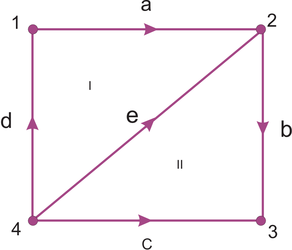
(31)

and

$$B_{I}:=Z_{e}Z_{a}^{-1}Z_{d}^{-1},\hskip 28.45274ptB_{II}:=Z_{c}Z_{b}^{-1}Z_{e}^{-1}.$$

(32)

Finally we note that all Kitaev states on a given graph, corresponding to different decorations are related to each other by local unitary actions. In fact if we switch the arbitrary orientation on a link $e_{ij}$, it means that the term $|\cdots\phi_{i}-\phi_{j},\cdots\rangle$ in (27) changes to $|\cdots\phi_{j}-\phi_{i},\cdots\rangle$ where the remaining parts of the state will remain intact. In view of (12), this switching is achieved by a local action of the square Hadamard operator $H^{2}$ on the edge $e$. We can thus write

$$|K_{G^{\sigma^{\prime}}}\rangle=\left(\bigotimes_{e:\sigma(e)\neq\sigma^{\prime}(e)}H^{2}_{e}\right)|K_{G^{\sigma}}\rangle.$$

(33)

Therefore all the Kitaev states with different decorations belong to the same class of states modulo local actions of square Hadamard operations.

In view of the shift invariance $\phi_{i}\longrightarrow\phi_{i}+\eta$, the Kitaev state has a hidden multiplicative factor which is in fact infinite. This symmetry can be removed by fixing a gauge (in the discrete case this is a finite factor which causes no problem). Therefore we will define the gauge-fixed Kitaev state, denoted by $|K^{0}_{G}\rangle$ as follows:

$$|K^{0}_{G}\rangle=\int d\phi_{1}d\phi_{2}...d\phi_{N}\delta(\phi_{1}+\phi_{2}+\cdots\phi_{N})\bigotimes_{e_{ij}}|\phi_{i}-\phi_{j}\rangle.$$

(34)

This gauge-fixed Kitaev state has still the same set of stabilizers. The same reasoning for the Kitaev state $|K_{G}\rangle$ also works here.

Let $G=(V,E,\sigma)$ be defined as in previous subsection. Now in addition to the modes on the edges, there are also modes on vertices, as in figure (4). On such a graph, there are thus two different sets of vertices, which we denote by $V$ (the ones on the nodes) and $V_{E}$ (the ones on the edges). Then the state $|\overline{K}_{G}\rangle$ is given by

$$|\overline{K}_{G}\rangle=\int d\phi_{1}d\phi_{2}...d\phi_{N}\bigotimes_{e_{ij}\in E}|\phi_{i}-\phi_{j}\rangle\bigotimes_{i\in V}|\phi_{i}\rangle,$$

(35)

where $e_{ij}$ is the edge which goes from vertex $i$ to $j$. As an example for the graph in figure (4), we have

$$|\overline{K}_{\cal G}\rangle=\int D\phi|\phi_{1}-\phi_{2},\phi_{2}-\phi_{3},\phi_{4}-\phi_{3},\phi_{4}-\phi_{1},\phi_{4}-\phi_{2}\rangle_{a,b,c,d,e}\otimes|\phi_{1},\phi_{2},\phi_{3},\phi_{4}\rangle_{1,2,3,4}.$$

(36)

The stabilizers of this extended Kitaev state are completely different from the simple Kitaev state. In fact they are: For each vertex $v\in V$,

$${C}_{v}:=X_{v}\prod_{e\in E_{v}}X_{e}^{\pm},$$

(37)

where the convention for the $\pm$ signs is the same as in Kitaev state and for each edge $e\in E$ which goes from $v_{1}$ to $v_{2}$,

$${D}_{e}:=Z_{e}^{-1}Z_{v_{1}}Z_{v_{2}}^{-1},$$

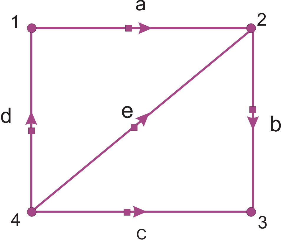
(38)

where again we have suppressed the continuous arguments of these stabilizers for ease of notation. For the example given in figure (4), some of the stabilizers are:

$\displaystyle C_{1}=X_{1}X_{a}X_{d}^{-1},\ \ \ C_{2}=X_{2}X_{a}^{-1}X_{e}^{-1}X_{b},\ \ \ D_{a}=Z_{1}Z_{a}^{-1}Z_{2}^{-1},\ \ \ D_{b}=Z_{2}Z_{b}^{-1}Z_{3},\cdots$

(39)

Finally we come to the definition of continuous variable weighted graph states. Here as in the qubit case we start with an initial product state of the form $|\Omega\rangle=|0\rangle_{p}^{\otimes V}$. However there is an important difference in that on each edge, instead of the simple $CZ$ operator, we can act by the $CZ(J)$ operator where the real parameter $J$ may depend on the edge. Therefore we obtain what we call a weighted graph state. Denoting the collection of all weights by $J$, we have

$$|\Psi_{G}(J)\rangle=\bigotimes_{e\in E}(CZ(J_{e}))|\Omega\rangle,$$

(40)

where $|\Omega\rangle=|0\rangle_{p}^{\otimes V}$. The explicit form of the state will then be given by

$$|\Psi_{G}(J)\rangle=\int D\phi e^{\sum_{<i,j>}J_{ij}\phi_{i}\phi_{j}}|\phi_{1},\cdots\phi_{N}\rangle,$$

(41)

where $N$ is the number of vertices and $<i,j>$ denotes the edge connecting the vertices $i$ and $j$ carrying weight $J_{ij}$. Note that in contrast to a decorated edge which is denoted by $e_{ij}$ (going from $i$ to $j$), a weighted edge is denoted by the symmetric symbol $\langle i,j\rangle$. According to (16), the stabilizers of this state will be of the form

$$K_{i}(t):=X_{i}(t)\prod_{j\in N_{i}}Z_{j}(J_{ij}t),\hskip 28.45274pt\forall\ i\in V,$$

(42)

where in the left hand side we have suppressed the dependence on the weights for simplicity.

We emphasize that definition of the Kitaev states and extended Kitaev states require the underlying graph to be decorated, while a graph state needs only a weighted graph for its unambiguous definition. We are now left with an important question of whether there is a simple relation between the above three kinds of states or not. The answer turns out to be positive and is explained in the next subsection.

Consider the extended Kitaev state corresponding to a decorated graph $G=(V,E,\sigma)$. The explicit form of the state is shown in (35). From (35) it is clear that if we project all the vertices in $V$ on the zero-momentum basis, we will arrive at the Kitaev state for the same graph. More explicitly we have

$$\langle\Omega|\overline{K}_{G^{\sigma}}\rangle=\frac{1}{\sqrt{(2\pi)^{|V|}}}|K_{G^{\sigma}}\rangle,$$

(43)

where $|\Omega\rangle=|0\rangle_{p}^{\otimes V}$, and we have explicitly indicated the decoration $\sigma$.
It is instructive to understand this in an alternative way, that is by showing that measurement in the momentum basis actually transforms the stabilizer set of the extended Kitaev state, i.e. $S(|\overline{K}_{G}^{\sigma}\rangle)$ to the stabilizer set of the Kitaev state, $S(|K_{G}^{\sigma}\rangle)$. From the stabilizer formalism we know that measurement of a state $|\Psi\rangle$ in the basis of an operator $M$, removes all the operators which do not commute with $M$ from the set $S(|\Psi\rangle)$ and leaves us with a smaller subset. This subset is generated by all the original generators or their products thereof which commute with $M$. Having this in mind, it is straightforward to see that measurement in the momentum (the $X$ basis) leaves all the vertex stabilizers $C_{v}$ intact (except of course removing the vertex $X_{v}$ from it), hence changing it to $A_{v}$ as in (28). However since $X_{v}$ does not commute with $Z_{v}$, measurements of all the vertices remove all the generators $D_{e}$. The only combinations which survive this elimination will be their product around any faces. These are nothing but the operators $B_{f}$ for all faces, which are just the right stabilizers of $|K_{G^{\sigma}}\rangle$.

Let us now study the relation between the extended Kitaev states and graph states. It turns out that there is a simple relation between the two only if the weights of the edges incident on each vertex add up to zero, that is, if

$$\sum_{j}J_{ij}=0,\hskip 28.45274pt\forall i.$$

(44)

Since $J_{ij}=J_{ji}$, this means also that $\sum_{i}J_{ij}=0$. In such a case we can convert an extended Kitaev state to a weighted graph state on the same graph by suitable measurements on the edges. To this end we proceed as follows: Let us project each edge $e_{ij}$ of the extended Kitaev state on the state $\langle\beta_{2}(t_{ij})|$ defined in (22).

Let $\langle\beta_{2}({\bf t})|:=\prod_{e_{ij}}\langle\beta_{2}(t_{ij})|$, then we have

$$\langle\beta_{2}({\bf t})|\overline{K}_{G}\rangle=\int D\phi e^{\sum_{e_{ij}}-it_{ij}(\phi_{i}-\phi_{j})^{2}}|\phi_{1},\cdots\phi_{N}\rangle.$$

(45)

If we choose the parameters $t_{ij}$ of quadratures so that $\sum_{i}t_{ij}=\sum_{j}t_{ij}=0$, we find

$$\langle\beta_{2}({\bf t})|\overline{K}_{G}\rangle=\int D\phi e^{\sum_{<i,j>}it_{ij}\phi_{i}\phi_{j}}|\phi_{1},\cdots\phi_{N}\rangle=:|\Psi_{G}({\bf it})\rangle,$$

(46)

which is a weighted graph state with weights $it_{ij}$ assigned to each edge $\langle i,j\rangle.$

Note that from the Kitaev state for the rectangular lattice $|K_{\square}\rangle$, the Kitaev state for any other graph $|K_{G}\rangle$ can be obtained simply by measurement of the edge modes in the momentum or coordinate bases. In fact projecting an edge mode on the zero-momentum state $|0\rangle_{p}$ removes that link from the graph while projecting it on the zero coordinate state $|0\rangle_{q}$ merges the two endpoints of that edge. These are shown in figure (5) and are proved as follows:

Let

$$|\psi\rangle=\int d\phi_{1}d\phi_{2}D^{\prime}\phi|\phi_{1}-\phi_{2}\rangle\prod_{i\in L}|\phi_{1}-\phi_{i}\rangle\prod_{j\in R}|\phi_{2}-\phi_{j}\rangle\cdots,$$

where $\cdots$ denotes all the edges which involve neither the vertex $1$ nor $2$. Projecting this state on the state ${}_{p}\langle 0|$ on the edge $\langle 1,2\rangle$, leaves us with

$$|\psi_{p}\rangle=\int d\phi_{1}d\phi_{2}D^{\prime}\phi\prod_{i\in L}|\phi_{1}-\phi_{i}\rangle\prod_{j\in R}|\phi_{2}-\phi_{j}\rangle\cdots,$$

(47)

which is nothing but the same Kitaev state with the edge $\langle 1,2\rangle$ totally removed. On the other hand projecting $|\psi\rangle$ on the state ${}_{q}\langle 0|$ on the edge $\langle 1,2\rangle$, leaves us with

	$\displaystyle|\psi_{q}\rangle$	$\displaystyle=$	$\displaystyle\int d\phi_{1}d\phi_{2}D^{\prime}\phi\delta(\phi_{1}-\phi_{2})\prod_{i\in L}|\phi_{1}-\phi_{i}\rangle\prod_{j\in R}|\phi_{2}-\phi_{j}\rangle\cdots$		(48)
		$\displaystyle=$	$\displaystyle\int d\phi_{1}D^{\prime}\phi\prod_{i\in L}|\phi_{1}-\phi_{i}\rangle\prod_{j\in R}|\phi_{1}-\phi_{j}\rangle\cdots,$		(49)

which means that the two endpoints of the edge $\langle 1,2\rangle$ have been merged together. With these two simple rules of deleting and merging one can obtain the Kitaev state of any graph starting from the one on the rectangular lattice. Figure (6) shows an important example in which measurements of some of the edges in the momentum basis (and hence removing them), transforms $|K_{\square}\rangle$ to the Kitaev state on the hexagonal lattice $|K_{H}\rangle$. Measurement of the same edges in the coordinate basis (and hence merging the two endpoints) produces a uniform lattice whose faces are triangles, hence a triangular lattice. This is in accord with the fact that the Hexagonal and Triangular lattice are dual to each other, a subject which will be explored further in the sequel.

Finally we use the well-known universality of cluster states proved in the context of measurement-based quantum computation [33, 34, 35, 36, 37, 38, 39] to state that both the Kitaev state $|K_{G}\rangle$ and the extended Kitaev state $|\overline{K}_{G}\rangle$ can be obtained by Gaussian measurements from a sufficiently large cluster state $|\Psi_{\square}\rangle$. The fact that the measurements need only be Gaussian is due to the fact that all these kinds of states are stabilized by subgroups of $W_{n}$ and hence they can be converted to each other by unitary operators belonging to the Clifford group. Using the well-known fact from MQC, that Clifford operators can be implemented by Gaussian measurements, we arrive at the proof of the above statement.

Consider a graph $G=(V,E)$ and a Hamiltonian $H_{0}$ defined on it without local potentials, $W_{i}(\phi)=0$. Let $W^{x}_{\widetilde{C}}$ be a closed loop on the dual graph, which is homologically trivial, (figure (7)) i.e. it is the boundary of an area. Since $W^{x}_{\widetilde{C}}$ can be written as a product of operators $A_{s}$, for $s$ inside the loop $\widetilde{C}$, we have

$$W^{x}_{\widetilde{C}}|K^{0}_{G}\rangle=|K^{0}_{G}\rangle,$$

(61)

or equivalently

$$\sum_{e\in{\widetilde{C}}}\widehat{P}_{e}|K^{0}_{G}\rangle=0.$$

(62)

Then in view of (57), this means that

$$\sum_{e_{i,j}\in{\widetilde{C}}}\langle V^{\prime}_{ij}(\phi_{i}-\phi_{j})\rangle=0.$$

(63)

This is a general non-trivial relation which is valid for any kind of interaction $V$ and without using the quantum formalism, it would have been difficult to obtain it. Note that the other kind of loop operator, $W^{z}_{C}$ defined as $W^{z}_{C}:=\prod_{i\in C}Z_{i}$ where $C$ is a loop in the graph, doesn’t lead to a non-trivial relation since in view of (56), insertion of this operator into the inner product leads to the quantity $\sum_{e_{ij}}(\phi_{i}-\phi_{j})$ which identically vanishes.

Denote the dual graph by $\widetilde{G}$. The vertices, edges and faces of $G$ are in one to one correspondence with the faces, edges and vertices of $\widetilde{G}$ respectively. For an oriented graph we should also choose a convention for choosing the orientations. We choose the convention that for each edge $e$ the dual $\widetilde{e}$ be such that the pair $(e,\widetilde{e})$ form a right handed frame, as in figure (8). In view of the form of stabilizers of the Kitaev states (28,29) and the relations (11), and the normalization of the state $|K_{G}\rangle$, we see that

$$|K_{\widetilde{G}}\rangle=(2\pi)^{\frac{|E|}{2}}H^{\otimes E}|K_{G}\rangle.$$

(64)

Note that contrary to the qubit case the duality relation is not an involution, that is, as shown in figure (8), the dual of the dual of an oriented graph is not the original graph, but the original graph with all the orientations reversed. This is in accord with the fact that $H^{2}\neq I$ and indeed the action of $H^{2}$ on all edges reverses their orientations. Consider now the partition function on $G$, with $\beta H$ as in (50). We have

$$Z(G,\{V\})=\langle\alpha|K_{G}\rangle=\frac{1}{(2\pi)^{\frac{|E|}{2}}}\langle\alpha|{H^{\dagger}}^{\otimes E}|K_{\widetilde{G}}\rangle=\frac{1}{(2\pi)^{\frac{|E|}{2}}}\langle\widetilde{\alpha}|K_{\widetilde{G}}\rangle,$$

(65)

where

$$|\widetilde{\alpha}\rangle=H|\alpha\rangle=H\int dxe^{-iV(x)}|x\rangle=\frac{1}{\sqrt{2\pi}}\int dxdye^{ixy-iV(x)}|y\rangle=\int dye^{-i\widetilde{V}(y)}|y\rangle,$$

(66)

where

$$e^{-i\widetilde{V}(y)}=\frac{1}{\sqrt{2\pi}}\int dxe^{ixy-iV(x)}.$$

(67)

This gives the following duality relation

$$Z(G,\{V\})=\frac{1}{(2\pi)^{\frac{|E|}{2}}}Z({\widetilde{G}},\{\widetilde{V}\}),$$

(68)

where $e^{-i\widetilde{V}}$ is the Fourier transform of $e^{-iV}$, as given in (67). An example of interest is when

$$V_{ij}(x)=\frac{1}{2}k_{ij}x^{2},$$

(69)

which leads to the following duality relation

$$Z(G,\{k_{ij}\})=\frac{1}{(2\pi)^{\frac{|E|}{2}}}\frac{1}{\sqrt{\prod_{ij}k_{ij}}}Z({\widetilde{G}},\{\frac{1}{k_{ij}}\}).$$

(70)

References

- [1] M. Van den Nest, W. Dur and H. J. Briegel, Phys. Rev. Lett. 98, 117207 (2007).
- [2] Van den Nest, W. Dur and H. J. Briegel, Phys. Rev. Lett. 100 110501 (2008) (Preprint arXiv:0708.2275).
- [3] L. Onsager, Phys. Rev. 65 117-149 (1944).
- [4] H. A. Kramers, G. H. Wannier. Phys. Rev. 60 252-262, 263-276 (1941).
- [5] B. Kaufman, L. Onsager, Phys. Rev. 76 1232-1243 (1949).
- [6] De las Cuevas , Dur, Briegel and Martin-Delgado, Phys. Rev. Lett. 102 230502 (2009) (Preprint arXiv:0812.3583).
- [7] G. De las Cuevas, W. Dur,H. J. Briegel and Martin-Delgado, New J. Phys. 12 043014 (2010) (Preprint arXiv:0911.2096).
- [8] Y. Xu, G. De las Cuevas, W. Dur, H. J. Briegel, M. A. Martin-Delgado, J. Stat. Mech. P02013 (2011).
- [9] G. De las Cuevas,W. Dur,M. Van den Nest and H. J. Briegel, J. Stat. Mech. P07001 (2009) (Preprint arXiv:0812.2368).
- [10] M. Van den Nest, W. Dur, R. Raussendorf and H. J. Briegel, Phys. Rev. A80 052334 (2009) (Preprint arXiv:0805.1214).
- [11] R. Hubener, M. Van den Nest, W. Dur and H. J. Briegel, J. Math. Phys. 50 083303 (2009) (Preprint arXiv:0812.2127).
- [12] S. Bravyi, R. Raussendorf, Phys. Rev. A 76, 022304 (2007).
- [13] M. Van den Nest, W. Dur, G. Vidal, H. J. Briegel, Phys. Rev. A 75, 012337 (2007).
- [14] R. Raussendorf and H. J. Briegel, Phys. Rev. Lett. 86, 5188 (2001).
- [15] D. Gross and J. Eisert, Phys. Rev. Lett. 98, 220503 (2007).
- [16] D. Gross, J. Eisert, N. Schuch, and D. Perez-Garcia, Phys. Rev. A 76, 052315 (2007).
- [17] D. Gross and J. Eisert, Phys. Rev. A 82, 040303(R) (2010).
- [18] G. K. Brennen and A. Miyake, Phys. Rev. Lett. 101, 010502 (2008).
- [19] X. Chen, B. Zeng, Z. C. Gu, B. Yoshida, and I. L. Chuang, Phys. Rev. Lett. 102, 220501 (2009).
- [20] C. E. Mora,M. Piani, A.Miyake, M. Van den Nest,W. Dur, and H. J. Briegel, Phys. Rev. A 81, 042315 (2010).
- [21] J. M. Cai, W. Dur, M. Van den Nest, A. Miyake, H. J. Briegel, Phys. Rev. Lett. 103, 050503 (2009)
- [22] Jianming Cai, Akimasa Miyake, Wolfgang Dur, Hans J. Briegel, Phys. Rev. A 82, 052309 (2010)
- [23] Wei-Bo Gao, Xing-Can Yao, Jian-Ming Cai, He Lu, Ping Xu, Tao Yang, Chao-Yang Lu, Yu-Ao Chen, Zeng-Bing Chen, Jian-Wei Pan, Nature Photonics 5, 117 (2011).
- [24] F. Barahona, J. Phys. A 15, 3241 (1982).
- [25] S. L. Braunstein and P. van Loock, Rev. Mod. Phys. 77, 513 (2005).
- [26] T. C. Ralph, A. Gilchrist, G. J. Milburn, W. J. Munro, and S. Glancy, Phys. Rev. A 68, 042319 (2003).
- [27] J. Zhang and S. L. Braunstein, Phys. Rev. A 73, 032318 (2006).
- [28] M. A. Nielsen, Phys. Rev. Lett. 93, 040503 (2004).
- [29] D. Gottesman, A. Kitaev, and J. Preskill, Phys. Rev. A 64, 012310 (2001).
- [30] R. L. Barnes, e-print arXiv:quant-ph/0405064.
- [31] P. van Loock, C. Weedbrook, and M. Gu, Phys. Rev. A 76, 032321 (2007).
- [32] E. Hostens, J. Dehaene, B. De Moor, Phys. Rev. A 71, 042315 (2005).
- [33] S. D. Bartlett, B. C. Sanders, S. L. Braunstein, and K. Nemoto, Phys. Rev. lett. 88 , 097904 (2002).
- [34] Nicolas C. Menicucci et al, Phys. Rev. Lett. 97, 110501 (2006).
- [35] M. Gu, C. Weedbrook, N. C. Menicucci, T. C. Ralph, and P. vanLoock, Phys. Rev. A. 79 , 062318 (2009).
- [36] Dan Browne and Hans Briegel, arXiv:0603226v2 (2006).
- [37] N. C. Menicucci, S. T. Flammia, and O. Pfister, Phys. Rev. Lett. 101, 130501 (2008).
- [38] S. T. Flammia, N. C. Menicucci, and O. Pfister, J. Phys. B 42, 114009 (2009).
- [39] R. Ukai, J.-I. Yoshikawa, N. Iwata, P. van Loock, and A. Furusawa, Phys. Rev. A 81, 032315 (2010).
- [40] S. Lloyd and S. L. Braunstein, Phys. Rev. Lett. 82, 1784 (1999).
- [41] S. Lloyd, Phys. Rev. Lett. 75, 346 (1995).
- [42] A. T. Sornborger and E. D. Stewart, Phys. Rev. A 60, 1956 (1999).
- [43] S. Sefi and P. van Loock, arXiv:1104.1148 (2011).
- [44] A. Kitaev, Ann. Phys. 303 (2003).
- [45] M. Hein, J. Eisert, and H. J. Briegel, Phys. Rev. A 69, 062311 (2004).
- [46] M. Van den Nest, A. Miyake, W. Dur, and H. J. Briegel, Phys. Rev. Lett. 97, 150504 (2006).