FERMILAB-PUB-12-015-T
LAPTh-003/12
Testing the Technicolor Interpretation
of CDF’s Dijet Excess at the LHC

The CDF Collaboration has reported evidence for a resonance near $150\,{\rm GeV}$ in the dijet-mass spectrum, $M_{jj}$, of $Wjj$ production. This is based on an integrated luminosity of $4.3\,{\rm fb}^{-1}$ [1] and updated with a total data sample of $7.3\,{\rm fb}^{-1}$ [2]. In Ref.  [2], the resonant dijet excess has a significance of $4.1\,\sigma$. The DØ Collaboration, on the other hand, published a search for this resonance based on $4.3\,{\rm fb}^{-1}$ that found no significant excess. Based on a $W+$Higgs boson production model, DØ reported a cross section for a potential signal of $0.82^{+0.83}_{-0.82}\,{\rm pb}$ and a 95% confidence level upper limit of $1.9\,{\rm pb}$ [3]. Analyzing its data with the same production model, CDF reported a signal rate of $3.0\pm 0.7\,{\rm pb}$ and a discrepancy between the two experiments of $2.5\,\sigma$ [4]. This discrepancy remains. The purpose of this paper is to urge that the LHC experiments, ATLAS and CMS, mount searches to test for the CDF dijet excess in the $Wjj$ and closely related channels. We do this in the context low-scale technicolor (LSTC), interpreting CDF’s dijet excess as the lightest technipion $\pi_{T}^{\pm,0}$ of this scenario, produced in association with $W^{\pm}$ in the decay $\rho_{T}^{\pm,0}\rightarrow W\pi_{T}$ [5]. The related channels supporting this interpretation are $\rho_{T}^{\pm}\rightarrow Z\pi_{T}^{\pm}$ and $W^{\pm}Z$. They require the fewest additional LSTC model assumptions to determine LHC production rates. We assume $\sqrt{s}=7\,{\rm TeV}$ and consider $\int{\cal L}dt=1$–$20\,{\rm fb}^{-1}$, an amount of data expected in 2012.¹¹ 1 A preliminary version of this paper was circulated as Ref. [6], assuming $\int{\cal L}dt=1$–$5\,{\rm fb}^{-1}$. The simulations we present here for various fixed luminosities may be applied to different ones by scaling the event rates. The question of raising the LHC collision energy to $8\,{\rm TeV}$ in 2012 is under consideration. This probably will not be advantageous for the LSTC signals discussed here and elsewhere because backgrounds, especially gluon-induced ones, grow faster with energy than do the signals.

Low-scale technicolor (LSTC) is a phenomenology based on walking technicolor [7, 8, 9, 10]. The gauge coupling $\alpha_{TC}$ must run very slowly for 100s of TeV above the TC scale $\Lambda_{TC}\sim$ several $100\,{\rm GeV}$ so that extended technicolor (ETC) can generate sizable quark and lepton masses while suppressing flavor-changing neutral current interactions [11]. This may be achieved, e.g., with technifermions belonging to higher-dimensional representations of the TC gauge group. The constraints of Ref. [11] on the number of ETC-fermion representations then imply that there will be technifermions in the fundamental TC representation as well. They are expected to condense at an appreciably lower energy scale than those belonging to the higher-dimensional representations and, thus, their technipions’ decay constant $F_{1}^{2}\ll F_{\pi}^{2}=(246\,{\rm GeV})^{2}$ [12]. Meson bound states of these technifermions will have a quarkonium-like spectrum with masses well below a TeV — greater than the previous Tevatron limit $M_{\rho_{T}}\mathrel{\hbox to0.0pt{\raise 2.20013pt\hbox{$>$}\hss}{\lower 2.20013pt\hbox{$\sim$}}}250\,{\rm GeV}$ [13, 14] and probably less than 600–700 GeV, a scale at which we believe the notion of “low-scale” TC ceases to make sense. The most accessible states are the lightest technivectors, $V_{T}=\rho_{T}(I^{G}J^{PC}=1^{+}1^{--})$, $\omega_{T}(0^{-}1^{--})$ and $a_{T}(1^{-}1^{++})$. Through their mixing with the electroweak bosons, they are readily produced as $s$-channel resonances via the Drell-Yan process in colliders. Technipions $\pi_{T}(1^{-}0^{-+})$ are accessed in $V_{T}$ decays. A central assumption of LSTC is that these lightest technihadrons may be treated in isolation, without significant mixing or other interference from higher-mass states. Also, we expect that (1) the lightest technifermions are $SU(3)$-color singlets, (2) isospin violation is small for $V_{T}$ and $\pi_{T}$, (3) $M_{\omega_{T}}\cong M_{\rho_{T}}$, and (4) $M_{a_{T}}$ is not far above $M_{\rho_{T}}$. This last assumption is made to keep the low-scale TC contribution to the $S$-parameter small. An extensive discussion of LSTC, including these points and precision electroweak constraints, is given in Ref. [15].

Walking technicolor has another important consequence: it enhances $M_{\pi_{T}}$ relative to $M_{\rho_{T}}$ so that the all-$\pi_{T}$ decay channels of the $V_{T}$ are likely to be closed [12]. Principal $V_{T}$-decay modes are $W\pi_{T}$, $Z\pi_{T}$, $\gamma\pi_{T}$, a pair of EW bosons (which can include one photon), and fermion-antifermion pairs [16, 17, 15]. If allowed by isospin, parity and angular momentum, $V_{T}$ decays to one or more weak bosons involve longitudinally-polarized $W_{L}/Z_{L}$, the technipions absorbed via the Higgs mechanism. These nominally strong decays are suppressed by powers of $\sin\chi=F_{1}/F_{\pi}\ll 1$. This is an important parameter in LSTC. It is a mixing factor that measures the amount that the lowest-scale technipion is the mass eigenstate $\pi_{T}$ ($\cos\chi$) and the amount that it is $W_{L}/Z_{L}$ ($\sin\chi$). Thus, each replacement of a mass-eigenstate $\pi_{T}$ by $W_{L}/Z_{L}$ in a $V_{T}$ decay amplitude costs a factor of $\tan\chi$. Decays to transversely-polarized $\gamma,W_{\perp},Z_{\perp}$ are suppressed by $g,g^{\prime}$. Thus, the $V_{T}$ are very narrow, $\Gamma(\rho_{T})\mathrel{\hbox to0.0pt{\raise 2.20013pt\hbox{$<$}\hss}{\lower 2.20013pt\hbox{$\sim$}}}1\,{\rm GeV}$ and $\Gamma(\omega_{T},a_{T})\mathrel{\hbox to0.0pt{\raise 2.20013pt\hbox{$<$}\hss}{\lower 2.20013pt\hbox{$\sim$}}}0.1\,{\rm GeV}$ for the masses considered here. These decays have striking signatures, visible above backgrounds within a limited mass range at the Tevatron and probably up to 600–700 GeV at the LHC [18, 19].

In Ref. [5] we proposed that CDF’s dijet excess is due to resonant production of $W\pi_{T}$ with $M_{\pi_{T}}=160\,{\rm GeV}$. We took $M_{\rho_{T}}=290\,{\rm GeV}$ and $M_{a_{T}}=1.1M_{\rho_{T}}=320\,{\rm GeV}$. Then, about 75% of the $W\pi_{T}$ rate at the Tevatron is due to $\rho_{T}\rightarrow W\pi_{T}$ and, of this, most of the $W$’s are longitudinally polarized.²² 2 About 70% of the $W\pi_{T}$ rate at the LHC is due to the $\rho_{T}$. The remainder is dominated by $a_{T}$ production. Its decay, and a small fraction of the $\rho_{T}$’s, involve $W_{\perp}$ production, which is generated by dimension-five operators [15]. These operators are suppressed by mass parameters $M_{V,A}$ that we take equal to $M_{\rho_{T}}$. The other LSTC parameters relevant to $W\pi_{T}$ production are $g_{\rho_{T}\pi_{T}\pi_{T}}$ and $\sin\chi$. The $\rho_{T}\to\pi_{T}\pi_{T}$ coupling $g_{\rho_{T}\pi_{T}\pi_{T}}$ is the same for all $\rho_{T}$ decays considered here and it is simply scaled from QCD; its Pythia default value is $\alpha_{\rho_{T}}=g_{\rho_{T}\pi_{T}\pi_{T}}^{2}/4\pi=2.16(3/N_{TC})$ with $N_{TC}=4$. We use $\sin\chi=1/3$. Using the LSTC model implemented in Pythia [16, 17, 20], we found $\sigma(\bar{p}p\rightarrow\rho_{T}\rightarrow W\pi_{T}\rightarrow Wjj)=2.2\,{\rm pb}$ ($480\,{\rm fb}$ after $W\rightarrow e\nu,\,\mu\nu$).³³ 3 This includes $B(\pi_{T}\rightarrow\bar{q}q)\simeq 90\%$ in the default Pythia $\pi_{T}$-decay table. Using CDF’s cuts, we closely matched its $M_{jj}$ distribution for signal and background. Motivated by the peculiar kinematics of $\rho_{T}$ production at the Tevatron and $\rho_{T}\rightarrow W\pi_{T}$ decay, we also suggested cuts intended to enhance the $\pi_{T}$ signal’s significance and to make $\rho_{T}\rightarrow Wjj$ visible. Several distributions of data in the excess region $115\,{\rm GeV}<M_{jj}<175\,{\rm GeV}$ published by CDF [2] — notably $M_{Wjj}$, $p_{T}(jj)$, $\Delta\phi$ and $\Delta R=\sqrt{(\Delta\eta)^{2}+(\Delta\phi)^{2}}$ — fit the expectations of the LSTC model very well. The background-subtracted $\Delta R$ distribution, in particular, has a behavior which, we believe, furnishes strong support for our dijet production mechanism.

The purpose of this paper is to propose and study ways to test for the CDF signal at the LHC. In Sec. 2 we review the kinematics of $\rho_{T},a_{T}\rightarrow W\pi_{T}$ and $Z\pi_{T}$ in LSTC. We also present an interesting new result: the nonanalytic behavior of $d\sigma/d(\Delta R$) and $d\sigma/d(\Delta\chi)$ at their thresholds, $(\Delta R)_{\rm min}$ and $(\Delta\chi)_{\rm min}$. Here $\Delta\chi$ is the opening angle between the $\pi_{T}$ decay jets in the $\rho_{T}$ rest frame. For massless jets, a good approximation, we find that $(\Delta R)_{\rm min}=(\Delta\chi)_{\rm min}=2\cos^{-1}(v)$, where $v=p_{\pi_{T}}/E_{\pi_{T}}$ is the $\pi_{T}$ velocity in the $\rho_{T}$ rest frame. This result, peculiar to production models such as LSTC in which a narrow resonance decays to another narrow resonance plus a $W$ or $Z$, provides measures of $v$ independent of $p/E$ and, hence, valuable corroboration of this type of production. In Sec. 3 we consider the $\rho_{T},a_{T}\rightarrow W\pi_{T}$ process. Its LHC cross section is $7.9\,{\rm pb}$ but, for CDF cuts, its backgrounds have increased by about a factor of ten. This makes testing for the dijet excess in this channel very challenging. We suggest cuts which enhance signal-to-background $(S/B)$ but which will still require a very good understanding of the backgrounds in $Wjj$ production and perhaps luminosity $\mathrel{\hbox to0.0pt{\raise 2.20013pt\hbox{$>$}\hss}{\lower 2.20013pt\hbox{$\sim$}}}10\,{\rm fb}^{-1}$ to observe, or exclude, this signal. In Sec. 4 we study $\rho_{T}^{\pm},a_{T}^{\pm}\rightarrow Z\pi_{T}^{\pm}$, whose cross section is $2.3\,{\rm pb}$ at $7\,{\rm TeV}$ ($155\,{\rm fb}$ after $Z\rightarrow e^{+}e^{-},\,\mu^{+}\mu^{-}$). This is the isospin partner of $\rho_{T}^{\pm},a_{T}^{\pm}\rightarrow W\pi_{T}^{0}$, so its cross section is rather confidently known. The $\ell^{+}\ell^{-}jj$ channel is free of QCD multijet and $\bar{t}t$ backgrounds and missing energy uncertainty. Reconstructing the $Zjj$ invariant mass and other signal distributions, particularly in $\Delta R$ and $\Delta\chi$, will benefit from this. Because of these features, we believe that the $Z\pi_{T}\rightarrow Zjj$ mode will be the surest test of CDF’s dijet signal at the LHC. In Sec. 5, we study $\rho_{T}^{\pm},a_{T}^{\pm}\rightarrow WZ$. The cross section for this mode is proportional to $\tan^{2}\chi$ times the $\rho_{T}^{\pm},a_{T}^{\pm}\rightarrow W^{\pm}\pi_{T}^{0}$ and $Z\pi_{T}^{\pm}$ rates, but enhanced by its greater phase space. We predict $\sigma(\rho_{T}^{\pm},a_{T}^{\pm}\rightarrow WZ)=1.3\,{\rm pb}$ for $\sin\chi=1/3$. In the all-leptons mode (with $e$’s and $\mu$’s), the rate is only $20\,{\rm fb}$, but jet-related uncertainties are entirely absent. The $WZ\to\ell^{+}\ell^{-}jj$ mode is also an interesting target of opportunity so long as $\sin\chi\mathrel{\hbox to0.0pt{\raise 2.20013pt\hbox{$>$}\hss}{\lower 2.20013pt\hbox{$\sim$}}}1/4$. The $\Delta R$ and $\Delta\chi$ distributions for $Z\to jj$ again provide support for our narrow LSTC-resonance production model. In short, one or both of the $Z\pi_{T}$ and $WZ$ modes should be accessible with the $\mathrel{\hbox to0.0pt{\raise 2.20013pt\hbox{$>$}\hss}{\lower 2.20013pt\hbox{$\sim$}}}20\,{\rm fb}^{-1}$ expected to be in hand by the end of 2012. Finally, we present in an appendix the details of calculations in Sec. 2 regarding the nonanalytic threshold behavior of the $\Delta\chi$ and $\Delta R$ distributions.

While the simulations of the CDF signal in this paper are made in the context of low-scale technicolor, their qualitative features apply to any model in which that signal is due to $\bar{q}q$ production of a narrow resonance decaying to a $W$ plus another narrow resonance. Several papers have appeared proposing such an $s$-channel mechanism [21, 22, 23, 24, 25, 26]. With similar resonance masses to our LSTC proposal, these models will have kinematic distributions like those we describe in Sec. 2. However, not all these models will have the $Zjj$ and $WZ$ signals of LSTC. There are also a large number of papers proposing that the CDF signal is due to production of a new particle (e.g., a leptophobic $Z^{\prime}$) that is not resonantly produced [27, 28, 29, 30, 31, 32, 33]. These “$t$-channel” models will not pass our kinematic tests.

The kinematics of $\rho_{T}\rightarrow W\pi_{T}$ at the Tevatron and LHC are a consequence of the basic LSTC feature that walking TC enhancements of $M_{\pi_{T}}$ strongly suggest $M_{\rho_{T}}<2M_{\pi_{T}}$ and, indeed, that the phase space for $\rho_{T}\rightarrow W\pi_{T}$ is quite limited [12, 34]. At the Tevatron, a $290\,{\rm GeV}$ $\rho_{T}$ is produced almost at rest, with almost no $p_{T}$ and very little boost along the beam direction. At the LHC, $p_{T}(\rho_{T})\mathrel{\hbox to0.0pt{\raise 2.20013pt\hbox{$<$}\hss}{\lower 2.20013pt\hbox{$\sim$}}}25\,{\rm GeV}$ and $\eta(\rho_{T})\mathrel{\hbox to0.0pt{\raise 2.20013pt\hbox{$<$}\hss}{\lower 2.20013pt\hbox{$\sim$}}}2.0$. Furthermore, the $\pi_{T}$ is emitted very slowly in the $\rho_{T}$ rest frame — $v\simeq 0.4$ for our assumed masses — so that its decay jets are roughly back-to-back in the lab frame. Thus, $p_{T}(\pi_{T})\mathrel{\hbox to0.0pt{\raise 2.20013pt\hbox{$<$}\hss}{\lower 2.20013pt\hbox{$\sim$}}}80\,{\rm GeV}$ and the $z$-boost invariant quantities $\Delta\phi$ and $\Delta R=\sqrt{(\Delta\eta)^{2}+(\Delta\phi)^{2}}$ are peaked at large values less than $\pi$.

These features of LSTC are supported by CDF’s $7.3\,{\rm fb}^{-1}$ data [2]. Figures 1–4 show distributions before and after background subtraction taken from the $115<M_{jj}<175\,{\rm GeV}$ region containing the dijet excess. The subtracted-data $M_{Wjj}$ signal has a narrow resonant shape quite near $290\,{\rm GeV}$. Unfortunately, the background peaks just below that mass so that one may be concerned that the subtracted data’s peak is due to underestimating the background. Also, as we expect, the subtracted $p_{T}(jj)$ data falls off sharply above $75\,{\rm GeV}$ and the subtracted $\Delta\phi$ data is strongly peaked at large values. Again, one may worry that these are artifacts of the peaks of the $M_{Wjj}$ background and the position of the $M_{jj}$ excess.

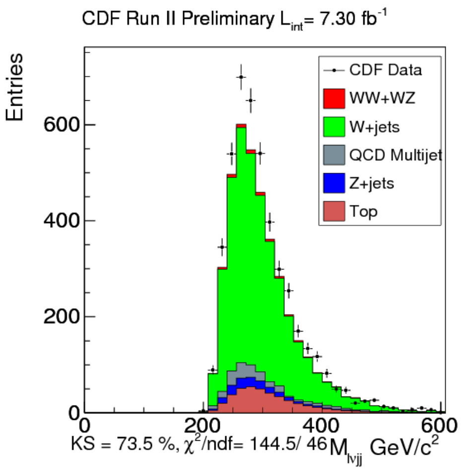
The background-subtracted $\Delta R$ distribution, however, is very interesting. It is practically zero for $\Delta R<2.25$, then rises sharply to a broad maximum before falling to zero again at $\Delta R\simeq 3.5$. This behavior, and a somewhat similar one we predict for $\Delta\chi$ are the main subject of this section. We will show that the threshold form of the $\Delta R$ and $\Delta\chi$ distributions provide direct measures of the velocity of the dijet system in the subprocess center-of-mass frame that are independent of measuring $p/E$ and, thus, are independent checks on the two-resonance topology of the dijet’s production mechanism.⁴⁴ 4 Recall that $\Delta\chi$ is defined in the $\rho_{T}$ rest frame, while $\Delta R$ is defined in the lab frame. If one wishes to remove the effect of $p_{T}(\rho_{T})$ on $\Delta R$, it should be defined in the $\rho_{T}$ frame. One might think that the corresponding $\Delta R_{\ell\ell}$ and $\Delta\chi_{\ell\ell}$ distributions from $Z\to\ell^{+}\ell^{-}$ would be similarly valuable. Unfortunately, because the dileptons come from real $Z$’s and our cuts make the background $Z$’s like the signal ones, $\Delta R_{\ell\ell}$ and $\Delta\chi_{\ell\ell}$ are indistinguishable from their backgrounds.

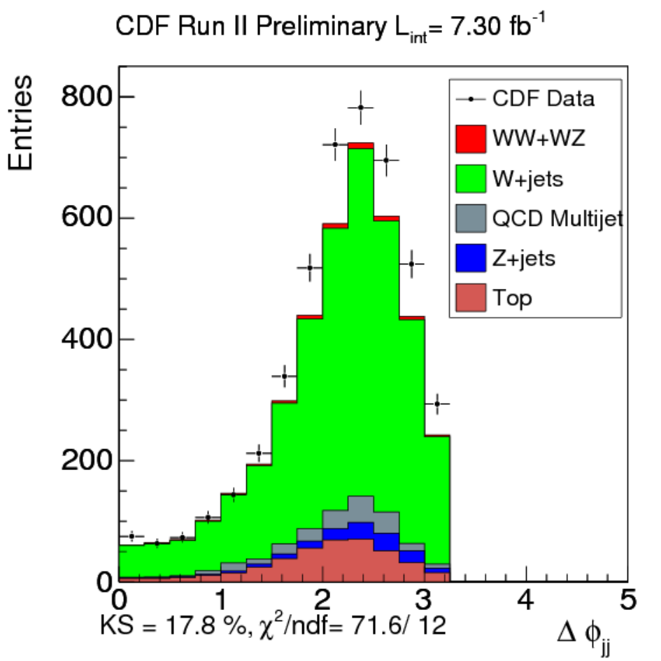
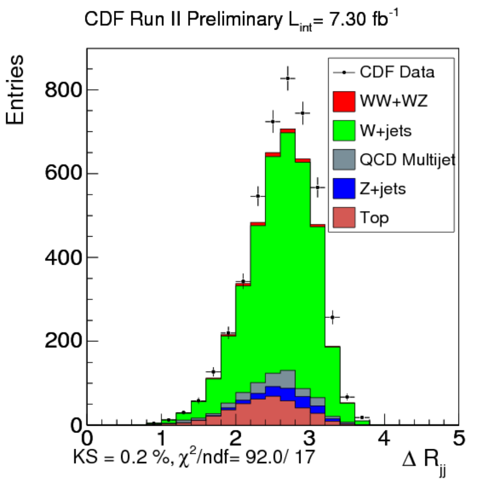
For our analysis, we assume the jets from $\pi_{T}$ decay are massless. We have examined the effect of including jet masses and found them to be unimportant. We will remark briefly on them at the end of this section. We first consider the dominant $\rho_{T}$ contribution to $W/Z\pi_{T}$ production, commenting on the $a_{T}$ contribution also at the end.

Define the angles $\theta$, $\theta^{*}$ and $\phi^{*}$ as follows: Choose the $z$-axis as the direction of the event’s boost; this is usually the direction of the incoming quark in the subprocess c.m. frame. In the $\rho_{T}$ rest frame, $\theta$ is the polar angle of the $\pi_{T}$ velocity ${\boldsymbol{v}}$, the angle it makes with the $z$-axis. Define the $xz$-plane as the one containing the unit vectors $\hat{\boldsymbol{z}}$ and $\hat{\boldsymbol{v}}$, so that $\hat{\boldsymbol{v}}=\hat{\boldsymbol{x}}\sin\theta+\hat{\boldsymbol{z}}\cos\theta$, and $\hat{\boldsymbol{y}}=\hat{\boldsymbol{z}}\times\hat{\boldsymbol{x}}$. Define a starred coordinate system in the $\pi_{T}$ rest frame by making a rotation by angle $\theta$ about the $y$-axis of the $\rho_{T}$ frame. This rotation takes $\hat{\boldsymbol{z}}$ into $\hat{\boldsymbol{z}}^{*}=\hat{\boldsymbol{v}}$ and $\hat{\boldsymbol{x}}$ into $\hat{\boldsymbol{x}}^{*}=\hat{\boldsymbol{x}}\cos\theta-\hat{\boldsymbol{z}}\sin\theta$. In this frame, let $\hat{\boldsymbol{p}}_{1}^{*}$ be the unit vector in the direction of the jet (parton) making the smaller angle with the direction of $\hat{\boldsymbol{v}}$. This angle is $\theta^{*}$; the azimuthal angle of ${\boldsymbol{p}}_{1}^{*}=-{\boldsymbol{p}}_{2}^{*}$ is $\phi^{*}$:

Note that, since $\pi_{T}\rightarrow\bar{q}q$ is isotropic in its rest frame, the distribution $d\sigma(\bar{q}q\rightarrow\rho_{T}\rightarrow Wjj)/d(\cos\theta^{*})=\sigma/2$, where $\sigma$ is the total subprocess cross section.

It is easier to consider the $d\sigma/d(\Delta\chi)$ distribution first. For massless jets,

The minimum value of $\Delta\chi$ occurs when $\theta^{*}=\pi/2$ (i.e., ${\boldsymbol{v}}\perp{\boldsymbol{p}}_{1}^{*}$), and so

From Eq. (2), it is easy to see that

i.e., the $\Delta\chi$ distribution has an inverse-square-root singularity at $\Delta\chi=(\Delta\chi)_{\rm min}=2\cos^{-1}(v)=2.23$ for our input masses, and falls sharply above there. This is illustrated in Fig. 5 where we plot this distribution for the primary partons and for the reconstructed jets. The low-side tail for the jets is an artifact of their reconstruction.

To understand this singularity better, it follows from Eq. (2) that $\Delta\chi$ may be expanded about $\cos\theta^{*}=0$ as

where $a$ is a positive $v$-dependent coefficient. Then, near $\cos\theta^{*}=0$, i.e., the $\Delta\chi$ threshold,

It is the simple one-variable Taylor expansion of $\Delta\chi$ in Eq. (5) that has caused this singularity.

The discussion of $d\sigma/d(\Delta R)$ for the LSTC signal shares some features with $d\sigma/d(\Delta\chi)$, though it it is qualitatively different. The $\Delta R$ distribution also vanishes below a threshold, $(\Delta R)_{\rm min}$, which is equal to $(\Delta\chi)_{\rm min}=2\cos^{-1}(v)$. This remarkable feature, derived in the appendix, can be understood simply as a consequence of the fact that the minimum of $\Delta R$ occurs when both jet rapidities vanish. In that case, $\Delta R=\Delta\phi=\Delta\chi$.

At threshold, however, the $\Delta R$ distribution is $\propto\sqrt{\Delta R-(\Delta\chi)_{\rm min}}$, not the inverse square root. As illustrated in Fig. 5, it rises sharply from threshold into a broad feature before decreasing. The measure of the $\pi_{T}$ velocity $v$ is given by the onset of the rise, not its peak. This is the behavior seen in the CDF data in Fig. 4, where the rise starts very near $2\cos^{-1}(v)=2.23$ for our input masses. Both the $\Delta\chi$ and $\Delta R$ distributions measure the $\pi_{T}$ velocity $v$ and, therefore, provide confirmations of the $\rho_{T}\rightarrow W\pi_{T}$ hypothesis which are independent of the background under the $M_{Wjj}$ resonant peak and of uncertainty in the $\kern 2.5pt\raise 0.77496pt\hbox{$/$}\kern-7.5ptE_{T}$ resolution as well.

The reason for this qualitative difference between the two distributions is that $d\sigma/\Delta\chi$ involves a one-dimensional trade of $\cos\theta^{*}$ for $\Delta\chi$, whereas $\Delta R$ is parametrized in terms of the three angles $\theta,\theta^{*},\phi^{*}$ in an intricate way, with all three being integrated over to account for the constraint defining $\Delta R$. In contrast to what happens in the $\Delta\chi$ case, the Jacobian singularity at the threshold is “antidifferentiated” twice, hence its comparatively lower strength. Using a Fadeev-Popov-like trick, the $\Delta R$ distribution can be written

The function $f(\cos\theta,\cos\theta^{*},\cos\phi^{*})$ is shown in the appendix to have its absolute minimum at $\cos\theta=\cos\theta^{*}=\cos\phi^{*}=0$, for which its value is equal to $(\Delta\chi)_{\rm min}$. Near its minimum it is locally parabolic and its Taylor expansion is

The positive $v$-dependent coefficients $b_{\theta},b_{\theta^{*}}$ and $b_{\phi^{*}}$ are also given in the appendix, Eq. (27). For $\Delta R$ close to $(\Delta\chi)_{\rm min}$, this expansion can be used to approximate Eq. (7). In a similar way as for the $\Delta\chi$ distribution, integrating first over $\cos\theta^{*}$ generates the appearance of a Jacobian inverse square root singularity $\propto[2(\Delta R-(\Delta\chi)_{\rm min})-(b_{\theta}\cos^{2}\theta+b_{\phi^{*}}\cos^{2}\phi^{*})]^{-1/2}$. The two remaining integrations over $\cos\theta$ and $\cos\phi^{*}$ were trivial in the $\Delta\chi$ case as the integrand did not depend on them, but this is not so for $\Delta R$ which involves a double integration over a restricted angular phase space defined by

Performing the integral in Eq. (7) near $(\Delta R)_{\rm min}=(\Delta\chi)_{\rm min}$ yields a result $\propto\sqrt{\Delta R-(\Delta\chi)_{\rm min}}$.

We have examined the effect of finite jet masses (as opposed to jet reconstruction and energy resolution) on the threshold values of the $\Delta R$ and $\Delta\chi$ distributions and the extraction of the $\pi_{T}$ velocity $v$ from them. Our jets (which include $b$-jets) have masses $\mathrel{\hbox to0.0pt{\raise 2.20013pt\hbox{$<$}\hss}{\lower 2.20013pt\hbox{$\sim$}}}10\,{\rm GeV}$. Assuming, for simplicity, equal jet masses and denoting by $u=\sqrt{1-4M_{\rm jet}^{2}/M_{\pi_{T}}^{2}}$ the jet velocity in the $\pi_{T}$ rest frame, the corrected $(\Delta\chi)_{\rm min}(u)$ is

This is less than the massless $(\Delta\chi)_{\rm min}$ by half a percent for $M_{\rm jet}=15\,{\rm GeV}$.

Finally, as noted, the $a_{T}$ accounts for about 25–30% of $W\pi_{T}$ production. This decay gives a $\pi_{T}$ velocity of 2.00 in the $a_{T}$ rest frame and $(\Delta\chi)_{\rm min}=2.00$. The effect is clearly visible in the $\Delta\chi$ and $\Delta R$ distributions for the primary parton in Fig. 5, but is washed out by the low-end tails for the reconstructed jets. We believe that the low and high-end tails are due to the two $\pi_{T}$ jets fragmenting to three jets and the two leading jets being closer or farther apart than the original pair.

As a reminder, we assumed $M_{\rho_{T}}=290\,{\rm GeV}$, $M_{a_{T}}=1.1M_{\rho_{T}}=320\,{\rm GeV}$, $M_{\pi_{T}}=160\,{\rm GeV}$ and $\sin\chi=1/3$ to describe the CDF dijet excess. The Tevatron cross section is $2.2\,{\rm pb}$. At the LHC, these parameters give $\sigma(W\pi_{T})=7.9\,{\rm pb}$ ($1.7\,{\rm pb}$ for $W\rightarrow e\nu,\,\mu\nu$). About 70% of the LHC rate is due to the $\rho_{T}$; the $\rho_{T}$ and $a_{T}$ interference is very small. For such close masses, it is not possible to resolve the two resonances in the $M_{Wjj}$ spectrum.

This past summer, the ATLAS Collaboration published dijet spectra for $1.02\,{\rm fb}^{-1}$ of $Wjj$ data with exactly two jets and with two or more jets passing selection criteria [35]. The ATLAS cuts, designed to be as close to CDF’s as possible, were: one isolated electron with $E_{T}>25\,{\rm GeV}$ or muon with $p_{T}>20\,{\rm GeV}$ and rapidity $|\eta_{\ell}|<2.5$; $\kern 2.5pt\raise 0.77496pt\hbox{$/$}\kern-7.5ptE_{T}>25\,{\rm GeV}$ and $M_{T}(W)>40\,{\rm GeV}$; two (or more) jets with $p_{T}>30\,{\rm GeV}$ and $|\eta_{j}|<2.8$; and $p_{T}(jj)>40\,{\rm GeV}$ and $\Delta\eta<2.5$ for the two leading jets. The $M_{jj}$ distribution for the two-jet data is shown in Fig. 6. There is no evidence of CDF’s dijet excess near $150\,{\rm GeV}$ nor even of the standard model $WW/WZ$ signal near $80\,{\rm GeV}$. This is what we anticipated in Ref. [6] because of the great increase in $Wjj$ backgrounds at the LHC relative to the Tevatron. On the other hand, it is noteworthy and encouraging for future prospects that the ATLAS background simulation appears to fit the data well.

In Fig. 6 we also show an updated version of our simulation of the LSTC $M_{jj}$ signal and backgrounds at the LHC for $\int{\cal L}dt=1.0\,{\rm fb}^{-1}$. ATLAS’s cuts were used except that we required $p_{T}(\ell)>30\,{\rm GeV}$.⁵⁵ 5 Backgrounds were generated at matrix-element level using ALPGENv213 [36], then passed to Pythiav6.4 for showering and hadronization. We use CTEQ6L1 parton distribution functions and a factorization/renormalization scale of $\mu=2M_{W}$ throughout. For the dominant $W+$jets background we generate $W+2j$ (excl.) plus $W+3j$ (inc.) samples, matched using the MLM procedure [37] (parton level cuts are imposed to ensure that $W+0,1$ jet events cannot contribute). After matching, the overall normalization is scaled to the NLO $W+jj$ value, calculated with MCFMv6 [38]. After passing through Pythia, final state particles are combined into $(\eta,\phi)$ cells of size $0.1\times 0.1$, and the energy in each cell smeared with $\Delta E/E=1.0/\sqrt{E/{{\rm GeV}}}$. The energy of each cell rescaled to make it massless. Isolated photons and leptons ($e,\mu$) are removed, and all remaining cells with energy greater than $1\,{\rm GeV}$ are clustered into jets using FastJet (anti-kT algorithm, $R=0.4$) [39]. Finally, the quadratic ambiguity in the $W$ reconstruction was resolved by choosing the solution with the smaller $p_{z}(\nu)$. This tighter cut and our inability to include the data-driven QCD background account for our lower event rate compared to ATLAS. Despite this, the agreement between the two is quite good. In particular, our simulation shows that the CDF/ATLAS cuts cannot reveal the LSTC interpretation of the CDF signal at the LHC for any reasonable luminosity.⁶⁶ 6 Models of the CDF signal that are $gg$-initiated or involve large coupling to heavier quarks, e.g., Ref. [26, 31], are likely excluded by the ATLAS data.

To improve the signal-to-background, we examined a variety of cuts motivated by $\rho_{T}\rightarrow W\pi_{T}$ kinematics. Cuts quite similar to those we proposed in Ref. [5] typically cause the background to peak very near the dijet resonance. To get the signal off the peak (and more like the original CDF $M_{jj}$ excess [1]), we used the following cuts: lepton $p_{T}>30\,{\rm GeV}$ and rapidity $|\eta_{\ell}|<2.5$, $\kern 2.5pt\raise 0.77496pt\hbox{$/$}\kern-7.5ptE_{T}>25\,{\rm GeV}$, $M_{T}(W)>40\,{\rm GeV}$ and $p_{T}(W)>60\,{\rm GeV}$; exactly two jets with $p_{T1}>40\,{\rm GeV}$, $p_{T2}>30\,{\rm GeV}$, and $|\eta_{j}|<2.8$; and $p_{T}(jj)>45\,{\rm GeV}$, $\Delta\eta<1.2$; and $Q=M_{Wjj}-M_{jj}-M_{W}<100\,{\rm GeV}$. The $M_{jj}$ and $M_{Wjj}$ distributions are shown in Fig. 7 for $\int{\cal L}dt=5\,{\rm fb}^{-1}$. Counting events in the range $120<M_{jj}<170\,{\rm GeV}$ gives $S/\sqrt{B}=6.5$ but only $S/B=0.050$ for this luminosity. Likewise, the $\Delta R$ and $\Delta\chi$ signals are very small and not useful. This is not promising. Perhaps with 20–$30\,{\rm fb}^{-1}$ a convincing signal could be seen in the $Wjj$ data, but it would require a very good understanding of the backgrounds.

Observation of $\rho_{T}^{\pm},a_{T}^{\pm}\rightarrow Z\pi_{T}^{\pm}$, the isospin partner of the $W\pi_{T}^{0}$ decay mode, will be an important confirmation of CDF’s $Wjj$ signal. At the LHC, we predict $\sigma(\rho_{T}^{\pm},a_{T}^{\pm}\rightarrow Z\pi_{T}^{\pm})=2.5\,{\rm pb}$, lower than $\sigma(\rho_{T}^{\pm},a_{T}^{\pm}\rightarrow W\pi_{T}^{0})=3.4\,{\rm pb}$ because of the reduced phase space, $\propto p^{3}$. Then, $\sigma(\rho_{T}^{\pm},a_{T}^{\pm}\rightarrow Z\pi_{T}\rightarrow\ell^{+}\ell^{-}jj)=155\,{\rm fb}$ for $\ell=e$ and $\mu$. This is about 10% of the total $W\pi_{T}\rightarrow\ell\nu_{\ell}jj$ signal. We might, therefore, expect that $\sim 10$ times the luminosity needed for the $W\pi_{T}$ signal would be required for the same sensitivity to $Z\pi_{T}$. Actually, because there is no QCD multijet background nor $\kern 2.5pt\raise 0.77496pt\hbox{$/$}\kern-7.5ptE_{T}$ resolution to pollute the $Zjj$ data, the situation is better than this.

Figure 8 shows the $Z\pi_{T}$ signal and its background, almost entirely from $Z+{{\rm jets}}$, for $\int{\cal L}dt=20\,{\rm fb}^{-1}$. The cuts used here are: two electrons or muons of opposite charge with $p_{T}>30\,{\rm GeV}$, $|\eta_{\ell}|<2.5$, $60<M_{\ell^{+}\ell^{-}}<100\,{\rm GeV}$ and $p_{T}(Z)>50\,{\rm GeV}$; exactly two jets with $p_{T}>30\,{\rm GeV}$ and $|\eta_{j}|<2.8$; $p_{T}(jj)>40\,{\rm GeV}$, $\Delta\eta<1.75$ and $Q=M_{Zjj}-M_{jj}-M_{Z}<60\,{\rm GeV}$. This $Q$-cut is very important in reducing the background.⁷⁷ 7 $\rho_{T},a_{T}\rightarrow WZ\rightarrow\ell^{+}\ell^{-}jj$ is included in this simulation, but it is removed by the $Q$-cut. These give $S/\sqrt{B}=6.0$ and $S/B=0.13$ for the dijet signal in $120<M_{jj}<170\,{\rm GeV}$. The figure also shows the $M_{Zjj}$ distribution; it has $S/\sqrt{B}=5.8$ and $S/B=0.11$ for $250<M_{Zjj}<320\,{\rm GeV}$. These signal-to-background rates and the position of the dijet signal on the falling backgrounds are similar to those in Ref. [2]. Therefore, if our interpretation of the CDF dijet excess is correct, both $\pi_{T}\to jj$ and $\rho_{T}\to\ell^{+}\ell^{-}jj$ should be observable in the data to be collected at the LHC in 2012.

Figure 9 shows the $\Delta R$ and $\Delta\chi$ distributions for $\rho_{T},a_{T}\rightarrow Z\pi_{T}\rightarrow\ell^{+}\ell^{-}jj$. The skyscraper-shaped $\Delta\chi$ distribution is interesting. The background peaks at $\Delta\chi\simeq 2.3$, and appears rather symmetrical about this point except that its high side falls more rapidly above $2.7$ because $(\Delta\chi)_{\rm max}=\pi$. The signal’s $\Delta\chi$ distribution sits atop the skyscraper, concentrated in about 175 events in a Chrysler Building-like spire⁸⁸ 8 http://en.wikipedia.org/wiki/Chrysler$\textunderscore$Building at $\Delta\chi=2.2$–2.3, whereas the theoretical $(\Delta\chi)_{\rm min}=2\cos^{-1}(v)=2.31$ for $\rho_{T}\to Z\pi_{T}$. This is just as expected when the effects of jet reconstruction and $a_{T}\to Z\pi_{T}$ are taken into account; see Fig. 5. If the actual $\Delta\chi$ data, with our cuts, has the shape of our simulation, we believe the signal spire excess can be observed. Similar remarks apply to the shape and observability of the slightly broader $\Delta R$ distribution in Fig. 9.

Finally, the decay channel $\rho_{T}^{\pm},a_{T}^{\pm}\to W^{\pm}Z$ furnishes another important check on the LSTC hypothesis provided that $\sin\chi\mathrel{\hbox to0.0pt{\raise 2.20013pt\hbox{$>$}\hss}{\lower 2.20013pt\hbox{$\sim$}}}1/4$. The dominant contribution, $\rho_{T}\to W_{L}Z_{L}$, has an angular distribution $\propto\sin^{2}\theta$ so that the production is fairly central. We expect $\sigma(\rho_{T},a_{T}\to WZ)/\sigma(\rho_{T},a_{T}\to W\pi_{T}^{0})\simeq(p(Z)/p(\pi_{T}))^{3}\,\tan^{2}\chi$. The Pythia rates are roughly consistent with this. For our input masses and $\sin\chi=({\textstyle{\frac{1}{4}}},{\textstyle{\frac{1}{3}}},{\textstyle{\frac{1}{2}}})$, we obtain

for $\ell=e,\mu$.

The $\rho_{T},a_{T}\to\ell^{+}\ell^{-}\ell^{\pm}\nu_{\ell}$ mode has been discussed in Refs. [18, 19]. It has the advantages of cleanliness and freedom from jet uncertainties (except $\kern 2.5pt\raise 0.77496pt\hbox{$/$}\kern-7.5ptE_{T}$ resolution). Standard-model $WZ$ production at the LHC peaks at $M_{WZ}=300\,{\rm GeV}\simeq M_{\rho_{T}}$ and this is the dominant background to the $3\ell\nu$ signal. The DØ collaboration searched for this channel for the standard LSTC parameters including $\sin\chi=1/3$, and excluded it at 95% C.L. up to $M_{\rho_{T}}\simeq 400\,{\rm GeV}$ so long as the $\rho_{T}\to W\pi_{T}$ channel is closed [40]. The CMS Collaboration recently reported a search for a sequential standard model $W^{\prime}$ and for $\rho_{T},a_{T}\to WZ\to 3\ell\nu$ using $1.15\,{\rm fb}^{-1}$ of $7\,{\rm TeV}$ data [41]. The $M_{WZ}$ spectrum and $M_{\rho_{T}}$ vs. $M_{\pi_{T}}$ exclusion plot are shown in Fig. 10. Standard LSTC parameters, including $\sin\chi=1/3$ were used for this plot. Extrapolating it rules out ($M_{\rho_{T}}=290\,{\rm GeV},\,M_{\pi_{T}}=180\,{\rm GeV}$) at 95%. It appears that 5–$10\,{\rm fb}^{-1}$ will be sufficient to exclude our CDF/LSTC mass point of $(290,160)\,{\rm GeV}$ for $\sin\chi\mathrel{\hbox to0.0pt{\raise 2.20013pt\hbox{$>$}\hss}{\lower 2.20013pt\hbox{$\sim$}}}1/3$.

The dominant background to $\rho_{T},a_{T}\to WZ\to\ell^{+}\ell^{-}jj$ is $Z+{\rm jets}$. As can be inferred from Fig. 6 for $Wjj$ production with ATLAS/CDF cuts, the signal will sit at the top of the $M_{jj}$ spectrum. This is what makes the dijet signal in $WW/WZ\to\ell\nu jj$ so difficult to see. On the plus side, since the LSTC and standard model diboson processes have very similar production characteristics, the two signals can be seen with the same cuts and will coincide. We simulated this mode and found what may be a promising set of cuts to extract the $W\to jj$ signal. The basic cuts used for the $Zjj$ signal in Sec. 4 were adopted except that we required $p_{T}(Z)>100\,{\rm GeV}$, $p_{T}(jj)>70\,{\rm GeV}$ and $110<Q=M_{Zjj}-M_{W}-M_{Z}<150\,{\rm GeV}$. The mass distributions for $\sin\chi=1/3$ are shown in Fig. 11 for $\int{\cal L}dt=20\,{\rm fb}^{-1}$. The LSTC signal more than doubles the number of standard model $W\to jj$ events in the $M_{jj}$ distribution and it appears that the dijet signal should be observable with such a data set. Including the standard diboson events gives $S/\sqrt{B}=4.1$ and $S/B=0.10$ for $60<M_{jj}<100\,{\rm GeV}$. The $M_{Zjj}$ signal is problematic, but it may be possible to combine its significance with that for $\rho_{T},a_{T}\to Z\pi_{T}\to\ell^{+}\ell^{-}jj$. The $\Delta R$ and $\Delta\chi$ distributions are in Fig. 12. The narrow LSTC signal and the diboson contribution both peak very near $(\Delta\chi)_{\rm min}=2\cos^{-1}(v_{W})=1.21$ and they should be observable as well.

We are grateful to K. Black, T. Bose, P. Catastini, V. Cavaliere, C. Fantasia and M. Mangano for valuable conversations and advice. This work was supported by Fermilab operated by Fermi Research Alliance, LLC, U.S. Department of Energy Contract DE-AC02-07CH11359 (EE and AM) and in part by the U.S. Department of Energy under Grant DE-FG02-91ER40676 (KL). KL’s research was also supported in part by Laboratoire d’Annecy-le-Vieux de Physique Theorique (LAPTh) and the CERN Theory Group and he thanks LAPTh and CERN for their hospitality.

References

- [1] CDF Collaboration, T. Aaltonen et. al., “Invariant Mass Distribution of Jet Pairs Produced in Association with a W boson in ppbar Collisions at sqrt(s) = 1.96 TeV,” Phys. Rev. Lett. 106 (2011) 171801, 1104.0699.
- [2] CDF Collaboration http://www-cdf.fnal.gov/physics/ewk/2011/wjj/73.html.
- [3] D0 Collaboration, V. M. Abazov, “Bounds on an anomalous dijet resonance in W+jets production in ppbar collisions at sqrts =1.96 TeV,” Phys. Rev. Lett. 107 (2011) 011804, 1106.1921.
- [4] A. Annovi, “Physics Beyond the Standard Model, talk at Lepton-Photon 2011, Mumbai, India.” 2011.
- [5] E. J. Eichten, K. Lane, and A. Martin, “Technicolor at the Tevatron,” Phys. Rev. Lett. 106 (2011) 251803, 1104.0976.
- [6] E. Eichten, K. Lane, and A. Martin, “Testing CDF’s Dijet Excess and Technicolor at the LHC,” 1107.4075.
- [7] B. Holdom, “Raising the sideways scale,” Phys. Rev. D24 (1981) 1441.
- [8] T. W. Appelquist, D. Karabali, and L. C. R. Wijewardhana, “Chiral hierarchies and the flavor changing neutral current problem in technicolor,” Phys. Rev. Lett. 57 (1986) 957.
- [9] K. Yamawaki, M. Bando, and K.-i. Matumoto, “Scale invariant technicolor model and a technidilaton,” Phys. Rev. Lett. 56 (1986) 1335.
- [10] T. Akiba and T. Yanagida, “Hierarchic chiral condensate,” Phys. Lett. B169 (1986) 432.
- [11] E. Eichten and K. D. Lane, “Dynamical Breaking of Weak Interaction Symmetries,” Phys. Lett. B90 (1980) 125–130.
- [12] K. D. Lane and E. Eichten, “Two Scale Technicolor,” Phys. Lett. B222 (1989) 274.
- [13] D0 Collaboration Collaboration, V. Abazov et. al., “Search for techniparticles in e+jets events at D0,” Phys.Rev.Lett. 98 (2007) 221801, hep-ex/0612013.
- [14] CDF Collaboration Collaboration, T. Aaltonen et. al., “Search for Technicolor Particles Produced in Association with a W Boson at CDF,” Phys.Rev.Lett. 104 (2010) 111802, 0912.2059.
- [15] K. Lane and A. Martin, “An Effective Lagrangian for Low-Scale Technicolor,” Phys. Rev. D80 (2009) 115001, 0907.3737.
- [16] K. Lane and S. Mrenna, “The collider phenomenology of technihadrons in the technicolor Straw Man Model,” Phys. Rev. D67 (2003) 115011, hep-ph/0210299.
- [17] E. Eichten and K. Lane, “Low-scale technicolor at the Tevatron and LHC,” Phys.Lett. B669 (2008) 235–238, 0706.2339.
- [18] G. Brooijmans et. al., “New Physics at the LHC: A Les Houches Report. Physics at Tev Colliders 2007 – New Physics Working Group,” 0802.3715.
- [19] G. Brooijmans et. al., “New Physics at the LHC. A Les Houches Report: Physics at TeV Colliders 2009 - New Physics Working Group,” 1005.1229.
- [20] T. Sjostrand, S. Mrenna, and P. Skands, “PYTHIA 6.4 physics and manual,” JHEP 05 (2006) 026, hep-ph/0603175.
- [21] C. Kilic and S. Thomas, “Signatures of Resonant Super-Partner Production with Charged-Current Decays,” Phys. Rev. D84 (2011) 055012, 1104.1002.
- [22] Q.-H. Cao et. al., “W plus two jets from a quasi-inert Higgs doublet,” JHEP 08 (2011) 002, 1104.4776.
- [23] C.-H. Chen, C.-W. Chiang, T. Nomura, and Y. Fusheng, “A light charged Higgs boson in two-Higgs doublet model for CDF anomaly,” 1105.2870.
- [24] J. Fan, D. Krohn, P. Langacker, and I. Yavin, “A Higgsophilic s-channel Z’ and the CDF W+2J Anomaly,” Phys. Rev. D84 (2011) 105012, 1106.1682.
- [25] D. K. Ghosh, M. Maity, and S. Roy, “R parity violating supersymmetric explanation for the CDF Wjj excess,” Phys. Rev. D84 (2011) 035022, 1107.0649.
- [26] J. F. Gunion, “A two-Higgs-doublet interpretation of a small Tevatron excess,” 1106.3308.
- [27] M. R. Buckley, D. Hooper, J. Kopp, and E. Neil, “Light Z’ Bosons at the Tevatron,” Phys. Rev. D83 (2011) 115013, 1103.6035.
- [28] J. Hewett and T. Rizzo, “Dissecting the Wjj Anomaly: Diagnostic Tests of a Leptophobic Z’,” 1106.0294v1.
- [29] R. Harnik, G. D. Kribs, and A. Martin, “Quirks at the Tevatron and Beyond,” Phys. Rev. D84 (2011) 035029, 1106.2569.
- [30] B. A. Dobrescu and G. Z. Krnjaic, “Weak-triplet, color-octet scalars and the CDF dijet excess,” 1104.2893v1.
- [31] A. E. Nelson, T. Okui, and T. S. Roy, “A unified, flavor symmetric explanation for the t-tbar asymmetry and Wjj excess at CDF,” Phys. Rev. D84 (2011) 094007, 1104.2030.
- [32] F. Yu, “A Z’ Model for the CDF Dijet Anomaly,” Phys. Rev. D83 (2011) 094028, 1104.0243.
- [33] K. Cheung and J. Song, “Baryonic Z’ Explanation for the CDF Wjj Excess,” Phys. Rev. Lett. 106 (2011) 211803, 1104.1375.
- [34] E. Eichten, K. D. Lane, and J. Womersley, “Finding low scale technicolor at hadron colliders,” Phys.Lett. B405 (1997) 305–311, hep-ph/9704455.
- [35] ATLAS Collaboration, “Invariant mass distribution of jet pairs produced in association with a leptonically decaying boson using of ATLAS data.” ATLAS-CONF-2011-097.
- [36] M. L. Mangano, M. Moretti, F. Piccinini, R. Pittau, and A. D. Polosa, “ALPGEN, a generator for hard multiparton processes in hadronic collisions,” JHEP 07 (2003) 001, hep-ph/0206293.
- [37] M. Mangano http://mlm.web.cern.ch/mlm/talks/lund-alpgen.pdf, 2004.
- [38] J. M. Campbell, R. K. Ellis, and C. Williams, “Vector boson pair production at the LHC,” JHEP 07 (2011) 018, 1105.0020.
- [39] M. Cacciari and G. P. Salam, “Dispelling the myth for the jet-finder,” Phys. Lett. B641 (2006) 57–61, hep-ph/0512210.
- [40] D0 Collaboration, V. M. Abazov et. al., “Search for a resonance decaying into WZ boson pairs in collisions,” Phys. Rev. Lett. 104 (2010) 061801, 0912.0715.
- [41] CMS Collaboration, “Search for the W’ (or techn-rho) to WZ.” CMS PAS EXO-11-041.