Iterative Approximate Byzantine Consensus
in Arbitrary Directed Graphs
Thanks: This report is a modified version of a previous technical report (Nitin Vaidya, Lewis Tseng, and Guanfeng Liang. Iterative Approximate Byzantine Consensus
in Arbitrary Directed Graphs. CoRR, abs/1201.4183, January 19 2012. http://arxiv.org/abs/1201.4183)
1 Introduction
In this paper, we explore the problem of iterative approximate Byzantine consensus in arbitrary directed graphs. In particular, we prove a necessary and sufficient condition for the existence of iterative Byzantine consensus algorithms. Additionally, we use our sufficient condition to examine whether such algorithms exist for some specific graphs.
Approximate Byzantine consensus [5] is a natural extension of original Byzantine Generals (or Byzantine consensus) problem [9]. The goal in approximate consensus is to allow the fault-free nodes to agree on values that are approximately equal to each other. There exist iterative algorithms for the approximate consensus problem that work correctly in fully connected graphs [5, 12] when the number of nodes exceeds , where is the upper bound on the number of failures. In [6], Fekete studies the convergence rate of approximate consensus algorithms. Ben-Or et al. develop an algorithm based on Gradcast to solve approximate consensus efficiently in a fully connected network [3].
There have been attempts at achieving approximate consensus iteratively in partially connected graphs. In [8], Kieckhafer and Azadmanesh examined the necessary conditions in order to achieve “local” convergence and performed a case study on global convergence in some special graphs. Later, they extended their work to asynchronous systems [2]. In [1], Azadmanesh et al. showed how to build a special network, called Partially Fully Connected Network, in which global convergence is achieved. Srinivasan and Azadmanesh studied the application of iterative approximate consensus in data aggregation, and developed an analytical approach using Markov chains [13, 14].
In [16], Sundaram and Hadjicostis explored Byzantine-fault tolerant distributed function calculation in an arbitrary network assuming a broadcast model. Under the broadcast model, every transmission of a node is received by all its neighbors. Hence, faulty nodes can send false data, but they have to send exactly the same piece of data to all their neighbors. They proved that distributed function calculation is possible if network connectivity is at least . Their algorithm maintains more “history” (a sequence of previous states) than the iterative algorithms considered in this paper.
In [18], Zhang and Sundaram studied the sufficient conditions for iterative consensus algorithm under “f-local” fault model. They also provided a construction of graphs satisfying the sufficient conditions.
LeBlanc and Koutsoukos [10] address a continuous time version of the Byzantine consensus problem in complete graphs. Recently, for the broadcast model, LeBlanc et al. have independently developed necessary and sufficient conditions for -fault tolerant approximate consensus in arbitrary graphs [17]; in [11] they have developed some sufficient conditions for correctness of a class of iterative consensus algorithms.
To the best of our knowledge, characterization of tight necessary and sufficient conditions for iterative approximate consensus in arbitrary directed graphs in the presence of Byzantine faults under point-to-point model is still an open problem. Iterative approximate consensus algorithms without any fault tolerance capability (i.e., ) in arbitrary graphs have been explored extensively. The proof of convergence presented in this paper is inspired by the prior work on non-fault-tolerant algorithms [4].
2 Preliminaries
2.1 Network Model
The network is modeled as a simple directed graph , where is the set of nodes, and is the set of directed edges between nodes in . We use the terms “edge” and “link” interchangeably. We assume that , since the consensus problem for is trivial. If a directed edge , then node can reliably transmit to node . For convenience, we exclude self-loops from , although every node is allowed to send messages to itself. We also assume that all edges are authenticated, such that when a node receives a message from node (on edge ), it can correctly determine that the message was sent by node . For each node , let be the set of nodes from which has incoming edges. That is, . Similarly, define as the set of nodes to which node has outgoing edges. That is, . By definition, and . However, we emphasize that each node can indeed send messages to itself. The network is assumed to be synchronous.
2.2 Failure Model
We consider the Byzantine failure model, with up to nodes becoming faulty. A faulty node may misbehave arbitrarily. Possible misbehavior includes sending incorrect and mismatching messages to different neighbors. The faulty nodes may potentially collaborate with each other. Moreover, the faulty nodes are assumed to have a complete knowledge of the state of the other nodes in the system and a complete knowledge of specification of the algorithm.
2.3 Iterative Approximate Byzantine Consensus
We consider iterative Byzantine consensus as follows:
- •
Up to nodes in the network may be Byzantine faulty.
- •
Each node starts with an input, which is assumed to be a single real number.
- •
Each node maintains state , with denoting the state of node at the end of the -th iteration of the algorithm. denotes the initial state of node , which is set equal to its input. Note that, at the start of the -th iteration (), the state of node is .
- •
The goal of an approximate consensus algorithm is to allow each node to compute an output in each iteration with the following two properties:
- –
Validity: The output of each node is within the convex hull of the inputs at the fault-free nodes.
- –
Convergence: The outputs of the different fault-free nodes converge to an identical value as .
- –
- •
Output constraint: For the family of iterative algorithms considered in this paper, output of node at time is equal to its state .
The iterative algorithms will be implemented as follows:
- •
At the start of -th iteration, , each node sends on all its outgoing links (to nodes in ).
- •
Denote by the vector of values received by node from nodes in at time . The size of vector is .
- •
Node updates its state using some transition function as follows, where is part of the specification of the algorithm:
Since the inputs are real numbers, and because we impose the above output constraint, the state of each node in each iteration is also viewed as a real number.
The function may be dependent on the network topology. However, as seen later, for convergence, it suffices for each node to know .
Observe that, given the state of the nodes at time , their state at time is independent of the prior history. The evolution of the state of the nodes may, therefore, be modeled by a Markov chain (although we will not use that approach in this paper).
We now introduce some notations.
- •
Let denote the set of Byzantine faulty nodes, where . Thus, the set of fault-free nodes is . 11 1 For sets and , contains elements that are in but not in . That is, .
- •
. is the largest state among the fault-free nodes (at time ). Recall that, due to the output constraint, the state of node at the end of iteration (i.e., ) is also its output in iteration .
- •
. is the smallest state among the fault-free nodes at time (we will use the phrase “at time ” interchangeably with “at the end of -th iteration”).
With the above notation, we can restate the validity and convergence conditions as follows:
- •
Validity: , and
- •
Convergence:
The output constraint and the validity condition together imply that the iterative algorithms of interest do not maintain a “sense of time”. In particular, the iterative computation by the algorithm, as captured in functions , cannot explicitly take the elapsed time (or ) into account.22 2 In a practical implementation, the algorithm may keep track of time, for instance, to decide to terminate after a certain number of iterations. Due to this, the validity condition for algorithms of interest here becomes:
| (1) |
In the discussion below, when we refer to the validity condition, we mean (1).
For illustration, below we present Algorithm 1 that satisfies
the output constraint.
The algorithm has been proved to achieve validity
and convergence in fully connected
graphs with [5, 12]. We will later address correctness of this
algorithm in arbitrary graphs.
Here, we assume that each node has at least incoming links. That is . Later, we will show that there is no iterative Byzantine consensus if this condition does not hold.
Algorithm 1
Steps that should be performed by each node in the
-th iteration are as follows. Note that the faulty nodes may
deviate from this specification.
Output of node at time is .
- 1.
Transmit current state on all outgoing edges.
- 2.
Receive values on all incoming edges (these values form vector of size ).
- 3.
Sort the values in in an increasing order, and eliminate the smallest values, and the largest values (breaking ties arbitrarily). Let denote the identifiers of nodes from whom the remaining values were received, and let denote the value received from node . Then, . By definition, . Note that if is fault-free, then . Define
(2) where
The “weight” of each term on the right side of (2) is , and these weights add to 1. Also, . For future reference, let us define as:
(3)
3 Necessary Condition
For an iterative Byzantine approximate consensus algorithm satisfying the output constraint, the validity condition, and the convergence condition to exist, the underlying graph must satisfy a necessary condition proved in this section. We now define relations and that are used frequently in our proofs.
Definition 1
For non-empty disjoint sets of nodes and ,
iff there exists a node that has at least incoming
links from nodes in , i.e., .
iff is not true.
Theorem 1
Let sets form a partition33 3 Sets are said to form a partition of set provided that (i) and when . of , such that
- •
,
- •
, and
- •
Then, at least one of the two conditions below must be true.
- •
- •
Proof:
The proof is by contradiction. Let us assume that a correct iterative consensus algorithm exists, and and . Thus, for any , , and , , Figure 1 illustrates the sets used in this proof.

Also assume that the nodes in (if is non-empty) are all faulty, and the remaining nodes, in sets , are fault-free. Note that the fault-free nodes are not necessarily aware of the identity of the faulty nodes.
Consider the case when (i) each node in has input , (ii) each node in has input , such that , and (iii) each node in , if is non-empty, has an input in the range .
At the start of iteration 1, suppose that the faulty nodes in (if non-empty) send to nodes in , send to nodes in , and send some arbitrary value in to the nodes in (if is non-empty). This behavior is possible since nodes in are faulty. Note that . Each fault-free node , sends to nodes in value in iteration 1.
Consider any node . Denote . Since , . Node will then receive from the nodes in , and values in from the nodes in , and from the nodes in .
Consider four cases:
- •
and are both empty: In this case, all the values that receives are from nodes in , and are identical to . By validity condition (1), node must set its new state, , to be as well.
- •
is empty and is non-empty: In this case, since , from ’s perspective, it is possible that all the nodes in are faulty, and the rest of the nodes are fault-free. In this situation, the values sent to node by the fault-free nodes (which are all in are all , and therefore, must be set to as per the validity condition (1).
- •
is non-empty and is empty: In this case, since , it is possible that all the nodes in are faulty, and the rest of the nodes are fault-free. In this situation, the values sent to node by the fault-free nodes (which are all in are all , and therefore, must be set to as per the validity condition (1).
- •
Both and are non-empty: From node ’s perspective, consider two possible scenarios: (a) nodes in are faulty, and the other nodes are fault-free, and (b) nodes in are faulty, and the other nodes are fault-free.
In scenario (a), from node ’s perspective, the non-faulty nodes have values in whereas the faulty nodes have value . According to the validity condition (1), . On the other hand, in scenario (b), the non-faulty nodes have values and , where ; so , according to the validity condition (1). Since node does not know whether the correct scenario is (a) or (b), it must update its state to satisfy the validity condition in both cases. Thus, it follows that .
Observe that in each case above for each node . Similarly, we can show that for each node .
Now consider the nodes in set , if is non-empty. All the values received by the nodes in are in , therefore, their new state must also remain in , as per the validity condition.
The above discussion implies that, at the end of the first iteration, the following conditions hold true: (i) state of each node in is , (ii) state of each node in is , and (iii) state of each node in is in . These conditions are identical to the initial conditions listed previously. Then, by induction, it follows that for any , , and . Since and contain fault-free nodes, the convergence requirement is not satisfied. This is a contradiction to the assumption that a correct iterative algorithm exists.
Corollary 1
Let be a partition of , such that , and and are non-empty. Then, either or .
Proof:
The proof follows by setting in Theorem 1.
While the two corollaries below are also proved in prior literature [7], we derive them again using the necessary condition above.
Corollary 2
The number of nodes must exceed for the existence of a correct iterative consensus algorithm tolerating failures.
Proof:
The proof is by contradiction. Suppose that , and consider the following two cases:
- •
: Suppose that is a partition of such that , and . Note that and are non-empty, and .
- •
: Suppose that is a partition of , such that and . Note that .
In both cases above, Corollary 1 is applicable. Thus, either or . For to be true, must contain at least nodes. Similarly, for to be true, must contain at least nodes. Therefore, at least one of the sets and must contain more than nodes. This contradicts our choice of and above (in both cases, size of and is ). Therefore, must be larger than .
Corollary 3
When , for each node , , i.e., each node has at least incoming links.
Proof:
The proof is by contradiction. Suppose that for some node , . Define set . Partition into two sets and such that and . Define . Thus, , and . Therefore, since and , . Also, since , .
This violates Corollary 1.
4 Useful Lemmas
Definition 2
For disjoint sets , denotes the set of all the nodes in that each have at least incoming links from nodes in . More formally,
With a slight abuse of notation, when , define .
Definition 3
For non-empty disjoint sets and , set is said to propagate to set in steps, where , if there exist sequences of sets and (propagating sequences) such that
- •
, , , and, for , .
- •
for ,
- *
,
- *
, and
- *
- *
Observe that and form a partition of , and for , . Also, when set propagates to set , length above is necessarily finite. In particular, is upper bounded by , since set must be of size at least for it to propagate to .
Lemma 1
Assume that satisfies Theorem 1. Consider a partition of such that and are non-empty, and . If , then set propagates to set .
Proof:
Since are non-empty, and , by Corollary 1, we have .
The proof is by induction. Define and . Thus and . Note that and are non-empty.
Induction basis: For some ,
- •
for , , and ,
- •
either or ,
- •
for , , and
Since , the induction basis holds true for .
Induction: If , then the proof is complete, since all the conditions specified in Definition 3 are satisfied by the sequences of sets and .

.
Now consider the case when . By assumption, , for . Define and . Our goal is to prove that either or . If , then the induction is complete. Therefore, now let us assume that and prove that . We will prove this by contradiction.
Suppose that . Define subsets as follows: , and . Figure 2 illustrates the sets used in this proof. Due to the manner in which ’s and ’s are defined, we also have . Observe that form a partition of , where are non-empty, and the following relationships hold:
- •
, and
- •
Rewriting and , using the above relationships, we have, respectively,
and
This violates the necessary condition in Theorem 1. This is a contradiction, completing the induction.
Thus, we have proved that, either (i) , or (ii) . Eventually, for large enough , will become , resulting in the propagating sequences and , satisfying the conditions in Definition 3. Therefore, propagates to .
Lemma 2
Assume that satisfies Theorem 1. For any partition of , where are both non-empty, and , at least one of the following conditions must be true:
- •
propagates to , or
- •
propagates to
Proof:
Consider two cases:
- •
: Then by Lemma 1, propagates to , completing the proof.
- •
: In this case, consider two sub-cases:
- –
propagates to : The proof in this case is complete.
- –
does not propagate to : Thus, propagating sequences defined in Definition 3 do not exist in this case. More precisely, there must exist , and sets and , such that:
- *
and , and
- *
for ,
- o
,
- o
, and
- o
.
- o
- *
and .
The last condition above violates the requirements for to propagate to .
Now , , and form a partition of . Since , by Lemma 1, propagates to .
Since , , and propagates to , it should be easy to see that propagates to . The proof is presented in the Appendix B for completeness.
- *
- –
5 Sufficiency
We prove that the necessary condition in Theorem 1 is sufficient. In particular, we will prove that Algorithm 1 satisfies validity and convergence conditions when the necessary condition is satisfied.
In the discussion below, assume that graph satisfies Theorem 1, and that is the set of faulty nodes in the network. Thus, the nodes in are fault-free. Since Theorem 1 holds for , all the subsequently developed corollaries and lemmas in Sections 3 and 4 also hold for .
Proof:
Consider the -th iteration, and any fault-free node . Consider two cases:
- •
: In (2), note that is computed using states from the previous iteration at node and other nodes. By definition of and , for all fault-free nodes . Thus, in this case, all the values used in computing are in the range . Since is computed as a weighted average of these values, is also within .
- •
: By Corollary 3, , and therefore, . When computing set , the largest and smallest values from are eliminated. Since at most nodes are faulty, it follows that, either (i) the values received from the faulty nodes are all eliminated, or (ii) the values from the faulty nodes that still remain are between values received from two fault-free nodes. Thus, the remaining values in () are all in the range . Also, is in , as per the definition of and . Thus is computed as a weighted average of values in , and, therefore, it will also be in .
Since , , the validity condition (1) is satisfied.
Lemma 3
Consider node . Let . Then, for ,
Specifically, for fault-free ,
Proof:
In (2), for each , consider two cases:
- •
Either or : Thus, is fault-free. In this case, . Therefore, .
- •
is faulty: In this case, must be non-zero (otherwise, all nodes are fault-free). From Corollary 3, . Then it follows that, in step 2 of Algorithm 1, the smallest values in contain the state of at least one fault-free node, say . This implies that . This, in turn, implies that
Thus, for all , we have . Therefore,
| (4) |
Since weights in Equation 2 add to 1, we can re-write that equation as,
| (5) | |||||
For non-faulty , , therefore,
| (6) |
Lemma 4
Consider node . Let . Then, for ,
Specifically, for fault-free ,
The lemma below uses parameter defined in (3).
Lemma 5
At time (i.e., at the end of the -th iteration), suppose that the fault-free nodes in can be partitioned into non-empty sets such that (i) propagates to in steps, and (ii) the states of nodes in are confined to an interval of length . Then,
| (7) |
Proof:
Since propagates to , as per Definition 3, there exist sequences of sets and , where
- •
, , , for , , and
- •
for ,
- *
,
- *
, and
- *
- *
Let us define the following bounds on the states of the nodes in at the end of the -th iteration:
| (8) | |||||
| (9) |
By the assumption in the statement of Lemma 5,
| (10) |
Also, and . Therefore, and .
The remaining proof of Lemma 5 relies on derivation of the three intermediate claims below.
Claim 1
For , for each node ,
| (11) |
Proof of Claim 1: The proof is by induction.
Induction basis: For some , , for each node , (11) holds. By definition of , the induction basis holds true for .
Induction: Assume that the induction basis holds true for some , . Consider . Observe that and form a partition of ; let us consider each of these sets separately.
- •
- •
Set : Consider a node . By definition of , we have that . Thus,
In Algorithm 1, values ( smallest and largest) received by node are eliminated before is computed at the end of -th iteration. Consider two possibilities:
- –
Value received from one of the nodes in is not eliminated. Suppose that this value is received from fault-free node . Then, by an argument similar to the previous case, we can set in Lemma 3, to obtain,
- –
Values received from all (there are at least ) nodes in are eliminated. Note that in this case must be non-zero (for , no value is eliminated, as already considered in the previous case). By Corollary 3, we know that each node must have at least incoming edges. Since at least values from nodes in are eliminated, and there are at least values to choose from, it follows that the values that are not eliminated44 4 At least one value received from the nodes in is not eliminated, since there are incoming edges, and only values are eliminated. are within the interval to which the values from belong. Thus, there exists a node (possibly faulty) from whom node receives some value – which is not eliminated – and a fault-free node such that
(12) Then by setting in Lemma 3 we have
- –
Thus, we have shown that for all nodes in ,
This completes the proof of Claim 1.
Claim 2
For each node ,
| (13) |
Proof of Claim 2:
Notice that by definition, . Then the proof follows by setting in the above Claim 1.
By a procedure similar to the derivation of Claim 2 above, we can also prove the claim below. The proof of Claim 3 is presented in the Appendix for completeness.
Claim 3
For each node ,
| (14) |
Now let us resume the proof of the Lemma 5. Note that . Thus,
| (15) | |||||
and
| (16) | |||||
| (17) | |||||
| (18) | |||||
| (19) |
This concludes the proof of Lemma 5.
Theorem 3
Suppose that satisfies Theorem 1. Then Algorithm 1 satisfies the convergence condition.
Proof:
Our goal is to prove that, given any , there exists such that
| (20) |
Consider -th iteration, for some . If , then the algorithm has already converged, and the proof is complete, with .
Now consider the case when . Partition into two subsets, and , such that, for each node , , and for each node , . By definition of and , there exist fault-free nodes and such that and . Thus, sets and are both non-empty. By Lemma 2, one of the following two conditions must be true:
- •
Set propagates to set . Then, define and . The states of all the nodes in are confined within an interval of length .
- •
Set propagates to set . Then, define and . In this case, states of all the nodes in are confined within an interval of length .
In both cases above, we have found non-empty sets and such that (i) is a partition of , (ii) propagates to , and (iii) the states in are confined to an interval of length . Suppose that propagates to in steps, where . By Lemma 5,
| (21) |
Since and , .
Let us define the following sequence of iteration indices55 5 Without loss of generality, we assume that . Otherwise, the statement is trivially true due to the validity shown in Theorem 2.:
- •
,
- •
for , , where for any given was defined above.
By repeated application of the argument leading to (21), we can prove that, for ,
| (22) |
For a given , by choosing a large enough , we can obtain
and, therefore,
| (23) |
For , by validity of Algorithm 1, it follows that
This concludes the proof.
6 Applications
In this section, we use the results in the previous sections to examine whether iterative approximate Byzantine consensus algorithm exists in some specific networks.
6.1 Core Network
Graph is said to be undirected iff implies that . We now define a class of undirected graphs, named core network.
Definition 4
Core Network: A graph consisting of nodes is said to be a core network if the following properties are satisfied: (i) it includes a clique formed by nodes in , such that , as a subgraph and, (ii) each node has links to all the nodes in . That is, (i) and , and (ii) , and , and .
It is easy to show that a core network satisfies the necessary condition in Theorem 1. Therefore, Algorithm 1 achieves approximate consensus in such network. We conjecture that a core network with has the smallest number of edges possible in any undirected network of nodes for which an iterative approximate consensus algorithm exists.
6.2 Hypercube
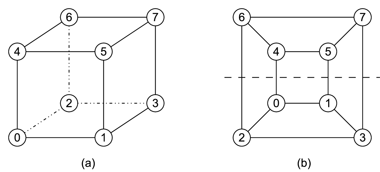
If the conensus algorithms are not required to satisfy the consatraints imposed on iterative algorithms in this paper, then it is known that conensus can be achieved in undirected graphs with connectivity [12]. However, connectivity of by itself is not sufficient for iterative algorithms of interest in this paper. For example, a -dimensional binary hypercube is an undirected graph consisting of nodes and has connectivity . However, a cut of this graph that removes edges along any one dimension fails to satisfy the necessary condition in Theorem 1, since each node has exactly one edge that belongs to the cut. Thus, each node in one part of the partition is neighbor to fewer than nodes in the other part, for any . Figure 3 illustrates such a partition for a 3-dimensional binary cube. Each undirected link in the figure represents two directed edges, namely, and .
6.3 Chord Network
A chord network is a directed graph defined as follows. This network is similar but not identical to the network in [15].
Definition 5
Chord network: A graph consisting of nodes is said to be a chord network if (i) , (ii) , iff , where . That is, for each node , .
The case when and results in a fully connected graph, which trivially satisfies Theorem 1. The following results can be shown for two other specific chord networks:
- •
When and , the chord network does not satisfy Theorem 1.
Let . Then the counter example is as follows:
Let node be faulty. Then consider and . This partition fails Theorem 1. Obviously, , since . However, , since and , which have size less than . Notice that this example also illustrate that connectivity of by itself is not sufficient in an directed and symmetric network.
- •
The Chord network with and satisfies Theorem 1.
7 Asynchronous Networks
The above results can be generalized to derive necessary and sufficient condition for (totally) asynchronous network under which the algorithm defined in [5] would work correctly. In essence, the primary change is that the requirement of incoming links in the definition of needs to be replaced by links. This implies that for each node when and , number of nodes, must exceed . The above results can also be generalized to the (partially) asynchronous model defined in Section 7 of [4] that allows for message delay of up to iterations.
Full details of the above generalizations will be presented in a future technical report.
8 Conclusion
This paper proves a necessary and sufficient condition for the existence of iterative approximate consensus algorithm in arbitrary directed graphs. As a special case, our results can also be applied to undirected graphs. We also use the necessary and sufficient condition to determine whether such iterative algorithms exist for certain specific graphs.
In our ongoing research, we are exploring extensions of the above results by relaxing some of the assumptions made in this work.
References
- [1] A.H. Azadmanesh and H. Bajwa. Global convergence in partially fully connected networks (pfcn) with limited relays. In Industrial Electronics Society, 2001. IECON ’01. The 27th Annual Conference of the IEEE, volume 3, pages 2022 –2025 vol.3, 2001.
- [2] M. H. Azadmanesh and R.M. Kieckhafer. Asynchronous approximate agreement in partially connected networks. International Journal of Parallel and Distributed Systems and Networks, 5(1):26–34, 2002. http://ahvaz.unomaha.edu/azad/pubs/ijpdsn.asyncpart.pdf
- [3] Michael Ben-Or, Danny Dolev, and Ezra N. Hoch. Simple gradecast based algorithms. CoRR, abs/1007.1049, 2010.
- [4] Dimitri P. Bertsekas and John N. Tsitsiklis. Parallel and Distributed Computation: Numerical Methods. Optimization and Neural Computation Series. Athena Scientific, 1997.
- [5] Danny Dolev, Nancy A. Lynch, Shlomit S. Pinter, Eugene W. Stark, and William E. Weihl. Reaching approximate agreement in the presence of faults. J. ACM, 33:499–516, May 1986.
- [6] A. D. Fekete. Asymptotically optimal algorithms for approximate agreement. In Proceedings of the fifth annual ACM symposium on Principles of distributed computing, PODC ’86, pages 73–87, New York, NY, USA, 1986. ACM.
- [7] Michael J. Fischer, Nancy A. Lynch, and Michael Merritt. Easy impossibility proofs for distributed consensus problems. In Proceedings of the fourth annual ACM symposium on Principles of distributed computing, PODC ’85, pages 59–70, New York, NY, USA, 1985. ACM.
- [8] R. M. Kieckhafer and M. H. Azadmanesh. Low cost approximate agreement in partially connected networks. Journal of Computing and Information, 3(1):53–85, 1993.
- [9] Leslie Lamport, Robert Shostak, and Marshall Pease. The Byzantine generals problem. ACM Trans. on Programming Languages and Systems, 1982.
- [10] Heath LeBlanc and Xenofon Koutsoukos. “Consensus in Networked Multi-Agent Systems with Adversaries,” 14th international conference on Hybrid systems: computation and control (HSCC), 2011.
- [11] (via personal communication with H. LeBlanc, January 19, 2012) Heath J. LeBlanc and Xenofon Koutsoukos. “Low Complexity Resilient Consensus in Networked Multi-Agent Systems with Adversaries,” to appear at 15th international conference on Hybrid systems: computation and control (HSCC), 2012.
- [12] Nancy A. Lynch. Distributed Algorithms. Morgan Kaufmann, 1996.
- [13] Satish M. Srinivasan and Azad H. Azadmanesh. Data aggregation in partially connected networks. Comput. Commun., 32:594–601, March 2009.
- [14] Satish M. Srinivasana and Azad H. Azadmanesh. Exploiting markov chains to reach approximate agreement in partially connected networks. In Symposium on Performance Evaluation of Computer and Telecommunication Systems, 2007.
- [15] I. Stoica, R. Morris, D. Liben-Nowell, D.R. Karger, M.F. Kaashoek, F. Dabek, and H. Balakrishnan. Chord: a scalable peer-to-peer lookup protocol for internet applications. Networking, IEEE/ACM Transactions on, 11(1):17 – 32, Feb. 2003.
- [16] S. Sundaram and C.N. Hadjicostis. Distributed function calculation via linear iterative strategies in the presence of malicious agents. Automatic Control, IEEE Transactions on, 56(7):1495 –1508, July 2011.
- [17] (via personal communication with S. Sundaram, January 18, 2012) Heath LeBlanc, Haotian Zhang, Shreyas Sundaram, and Xenofon Koutsoukos. “Consensus of Multi-Agent Networks in the Presence of Adversaries Using Only Local Information,” submitted to HiCoNs 2012.
- [18] Haotian Zhang and Shreyas Sundaram. Robustness of Information Diffusion Algorithms to Locally Bounded Adversaries. In CoRR, volume abs/1110.3843, 2011. http://arxiv.org/abs/1110.3843
Appendix A Proof of Claim 3
For each node ,
Proof:
Similar to the proof of claim 2, we will first prove the following claim:
Claim 4
For , for each node ,
| (24) |
Proof of Claim 4: The proof is by induction.
Induction basis: For some , , for each node , (24) holds. By definition of , the induction basis holds true for .
Induction: Assume that the induction basis holds true for some , . Consider . Observe that and form a partition of ; let us consider each of these sets separately.
- •
- •
Set : Consider a node . By definition of , we have that . Thus,
In Algorithm 1, values ( smallest and largest) received by node are eliminated before is computed at the end of -th iteration. Consider two possibilities:
- –
Value received from one of the nodes in is not eliminated. Suppose that this value is received from fault-free node . Then, by an argument similar to the previous case, we can set in Lemma 4, to obtain,
- –
Values received from all (there are at least ) nodes in are eliminated. Note that in this case must be non-zero (for , no value is eliminated, as already considered in the previous case). By Corollary 3, we know that each node must have at least incoming edges. Since at least values from nodes in are eliminated, and there are at least values to choose from, it follows that the values that are not eliminated are within the interval to which the values from belong. Thus, there exists a node (possibly faulty) from whom node receives some value – which is not eliminated – and a fault-free node such that
(25) Then by setting in Lemma 4 we have
- –
Thus, we have shown that for all nodes in ,
This completes the proof of Claim 4.
Now, we are able to prove Claim 3.
Proof of Claim 3:
Notice that by definition, . Then the proof follows by setting in the above Claim 4.
Appendix B Completing the proof of Lemma 2
The last line in the proof of Lemma 2 claims that:
“Since , , and propagates to , it should be easy to see that propagates to .”
We now prove the correctness of this claim.
Proof:
Recall that and form a partition of .
Let us define and . Thus, propagates to . Suppose that and are the propagating sequences in this case, with and forming a partition of .
Let us define and . Note that form a partition of . Now, and . Also, and form a partition of . Figure 4 illustrates some of the sets used in this proof.

- •
Define , and Also, , and .
Since and are a partition of , the nodes in belong to one of these two sets. Note that . Also, . Therefore, it follows that .
Thus, we have shown that, . Then it follows that .
- •
For , let us define and . Then following an argument similar to the above case, we can inductively show that, and . Due to the assumption on the length of the propagating sequence above, . Thus, there must exist , such that and, for , .
The sequences and form propagating sequences, proving that propagates to .
Appendix C Proof of Lemma 4
Proof:
In (2), for each , consider two cases:
- •
Either or : Thus, is fault-free. In this case, . Therefore, .
- •
is faulty: In this case, must be non-zero (otherwise, all nodes are fault-free). From Corollary 3, . Then it follows that, in step 2 of Algorithm 1, the largest values in contain the state of at least one fault-free node, say . This implies that . This, in turn, implies that
Thus, for all , we have . Therefore,
| (26) |
Since weights in Equation 2 add to 1, we can re-write that equation as,
| (27) | |||||
For non-faulty , , therefore,
| (28) |