Squeezing in driven bimodal Bose-Einstein Condensates: Erratic driving versus noise
Abstract
We study the interplay of squeezing and phase randomization near the hyperbolic instability of a two-site Bose-Hubbard model in the Josephson interaction regime. We obtain results for the quantum Zeno suppression of squeezing far beyond the previously found short time behavior. More importantly, we contrast the expected outcome with the case where randomization is induced by erratic driving with the same fluctuations as the quantum noise source, finding significant differences. These are related to the distribution of the squeezing factor, which has log-normal characteristics: hence its average is significantly different from its median due to the occurrence of rare events.
pacs
03.65.Xp, 03.75.Mn, 42.50.XaI Introduction
The effect of stochastic driving on unitary evolution has been a central theme of modern quantum mechanics. It is well established that quantum decay can be suppressed by frequent interventions, or measurements, or by the introduction of noise, via the Quantum Zeno Effect (QZE) [1, 2, 3, 4, 5, 6, 7, 8, 9, 10, 11, 12]. The modelling of the “interventions” as arising from a deterministic or from a noisy source are often used interchangeably [5, 6, 7, 8, 9]. This partially reflects the paradigm that the Langevin picture and the Master equation picture of the dynamics are equivalent.
Recent work considered the QZE suppression of interaction-induced squeezing in bimodal Bose-Einstein condensates [13, 14]. Since matter-wave squeezing is the key to the realization of atom interferometers below the standard quantum limit [15, 16, 17, 18, 19, 20], it is highly desirable to gain better understanding of its interplay with noise. Noise was shown to arrest the squeezing and build-up of many-body correlations in the large, multi-particle system, prepared with all particles occupying the odd superposition of the two-modes. In the Josephson regime [21] this preparation constitutes a hyperbolic saddle point, leading to a rapid squeezing [22, 23]. It was shown that the degree of squeezing and the associated phase diffusion [24, 25, 26, 27, 28, 29] could be controlled by a noisy modulation of the coupling between the modes, up to a full arrest via a Bose-stimulated QZE [13, 14].
In this work we attain two principle goals. (i) We extend the analytic understanding of the QZE suppression of squeezing to time-scales which are orders of magnitude longer than these of Ref. [13, 14], obtaining good agreement with numerical simulations. (ii) We challenge the fundamental paradigm of replacing quantum noise by deterministic erratic driving. Erratic driving can have non-trivial statistics, hence its typical results do not have to agree with the average behavior. This is demonstrated in our system by an important caveat resulting from the interplay of the nonlinear squeezing dynamics and the diffusive randomization by driving. While the early evolution under the influence of either noisy or erratic driving corresponds to the QZE of Ref. [13, 14], significant differences arise at later times. These differences are explained by a statistical analysis: As the squeezing is hyperbolic, while the driving induces diffusion, the resulting stretch distribution has log-normal characteristics, with rare events separating its mean from its median. The outcome of a typical erratic driving scenario is likely to reflect the median, and might be significantly different from the outcome of a full Feynman-Vernon averaging that is required for the description of quantum noise. Using semiclassical reasoning [30] we derive analytic expressions for the median and for the mean single-particle coherence, given the known normal statistics of the squeezing parameter.
In Section II we present the model driven Bose-Hubbard system, the pertinent initial conditions, and the relation between the squeezing parameter and the observed fringe visibility for Gaussian squeezed states. The coherence dynamics with and without noise are presented in Section III. The concept of erratic driving and its statistical analysis are introduced in Section IV and a short summary is provided in Section V.
II Modelling
We consider the dynamics generated by the two-mode Bose-Hubbard Hamiltonian (BHH) [21, 22, 23, 30] with an additional driving source,
| (1) |
where , , and . The and are bosonic annihilation and creation operators, respectively. The particle number operator in mode is . The total particle number is conserved. The dimensionless interaction parameter is . We note that the undriven two-mode BHH is known in nuclear physics as the Lipkin-Meshkov-Glick model [31, 32], and it has been also used to describe interacting spin systems [33] and magnetic molecules [34]. Our interest lies in the Josephson regime where [21], hence in the classical limit is a hyperbolic point. The driving source induces a fluctuating field which corresponds to the modulation of the barrier in a double-well realization of the two-mode BHH. We assume that this perturbation has a zero average and a short correlation time, such that upon averaging over time,
| (2) |
Hence the averaged dynamics is described by a Master equation which includes a term that generates angular diffusion around the axis:
| (3) |
where is the -particle density matrix. We preform numerical simulations of two possible scenarios: (a) Dynamics that is generated by the master equation; (b) Dynamics that is generated by a typical realization of [35]. Formally, the mixed state obtained in (a) can be regarded as the average over the pure states obtained in (b), provided that all possible realizations of are included.

One body coherence.– We consider an initial coherent preparation that is centered at the hyperbolic point . This corresponds to an -particle occupation of the anti-symmetric superposition of the two modes [22, 23]. The one-body coherence of the evolving state is characterized by the length of the Bloch vector . The symmetry of the Hamiltonian (1) and the initial preparation implies that so that the length of the Bloch vector is just the fringe visibility of an experimental multiple-shot interferometric measurement.
The Wigner function of the assumed coherent state preparation resembles a Gaussian centered at and having the angular width that corresponds to the minimum uncertainty of . A squeezed state is obtained by stretching along orthogonal major axes. The Wigner-Weyl representation of is , with corresponding expressions for and . Accordingly, the length of the Bloch vector for a squeezed state is
| (4) | |||||
| (5) |
where is the angular spreading. This is equivalent to a Gaussian squeezed state approximation, where the factorization is exact, allowing for the replacement of by . For the dynamical squeezing under study, this approximation is valid as long as . Thus, the error decreases for large and short evolution times.
III Loss of single-particle coherence due to squeezing
In the absence of noise the BHH (1) induces pure squeezing of the initial preparation at the Josephson rate , while the angle between the squeezing axes is twice the value of [13, 14]. Accordingly, the total angular variance of the Wigner function around the hyperbolic point grows initially as , leading to the loss of single-particle coherence as
| (6) |
As shown in Fig. 1a, Eq. (6) provides a good approximation for the numerically observed decay, beyond the previously used linearized form [13, 14].
IV Effect of noise
Here we would like to re-consider the scenario that has been analyzed in [13, 14]. Using the analogy to the standard QZE, the result that has been obtained there was an exponential decay
| (7) |
As seen in Fig. 1b, while this expression is accurate for the first few Josephson periods, it fails on longer time-scales. Long time accuracy may be improved using the semi-classical strategy of the previous paragraph. Thus, instead of applying the QZE sequence of projections directly to as done in [13, 14], we apply it here to the angular variance . One may visualize a sequence of squeezing intervals of duration wherein grows as before being reset by the noise. In the limit where , the spreading within each interval is quadratic in time, so that . Consequently
| (8) |
Comparison of Eq. (7) and Eq. (8) to the full numerical evolution (Fig. 1b) demonstrates great improvement over the short time result of Ref. [13, 14]. The simple exponential of Eq. (7) is only valid for where it can be approximated by a linear function. In comparison, Eq. (8) is valid for , after which decreases significantly below unity and the Gaussian approximation no longer holds.

V Erratic Driving vs. Noise
While Eq. (6) and Eq. (8) dramatically improve our quantitative understanding of the many-body QZE, far beyond the previously studied regime, our main focus here is to challenge the paradigm of replacing quantum noise by deterministic erratic driving. Erratic driving means that the Hamiltonian is time dependent due to some deterministic but fluctuating . An experimentalist can repeat one experiment many times with exactly the same , and determine the final quantum state. The experimentalist can also repeat the experiment with different realizations of and accumulate statistics.
By contrast, a noisy process as described by Eq. (3) can be viewed as arising from realizations that are induced by a bath. These realizations are not under experimental control: the individual cannot be reproduced from run to run. The best measurement the experimentalist can do already yields a density matrix , which we may call the average. In effect, it is Nature, rather than the experimentalist, who averages over . While the experimentalist considers individual realizations of , Nature averages over all realizations.
It is thus clear that in the case of erratic driving we should consider the statistics of , while in the case of a noisy driving only the averaged (i.e., the of the mixed state) has a physical meaning, as implied by the master equation.
Alternatively, erratic driving is aiming to emulate quantum noise by realizations that sample the ensemble of all possible paths. The naive expectation would be that for a reasonably large number of such realizations one would obtain a typical value which coincides with the true average. However, we show below that due to the interplay of Gaussian randomization and hyperbolic amplification, rare events which are missed by erratic driving play an important role in determining the final (typical) outcome of the squeezing in the presence of noise. Consequently, erratic driving sampling will typically differ substantially from the ideal average, even when the number of realizations is large.

VI Effect of erratic driving
Fig. 2 displays the time dependence of for a few representative realizations of erratic driving, out of a large sample of 2000 random scenarios. The mean, median, 25th and 75th percentiles, and the true average (from the master equation simulation) are indicated as well. As shown, the sample mean taken over the entire ensemble deviates from the “true” master equation result, and lies between the median and the true average.
In order to explain the observed difference between erratic driving and noise, we perform a statistical analysis of the evolving ensemble of squeezed states under erratic driving. In Fig. 3a we show the distribution of the squeezing axis direction and the degree of squeezing, with two extreme states. Each Gaussian squeezed state is represented by a pair of points along its long principle axis. The distance between the points is , which is two times the square root of the long axis variance. The latter obtained by the diagonalization of the variance matrix with . The empty internal ring corresponds to the minimal coherent state variance. We note that the principle axis direction is completely randomized with rare events of repeated stretching (the distant points).
The resulting distribution is log-wide as shown in Fig. 3d, with its median significantly smaller than its average. This log-normal statistics is explained as follows: for a given realization of the wavepacket undergoes a sequence of squeezing operations. Dividing the time into intervals of size , one realizes that the squeezing operations are uncorrelated, and can be regarded as a random sequence of stretching and un-stretching steps. Accordingly, the accumulated squeezing parameter is a sum of uncorrelated variables, and according to the central limit theorem it should have a normal distribution. From Eq. (5) it follows that will have log-wide distribution.
We can deduce the effective squeezing parameter for each realization from its single-particle coherence by inverting Eq. (5). The time evolution of the deduced distribution is shown in Fig. 3b, and a representative cross section is plotted in Fig. 3c. As expected, after a short transient of unfolding the squeezing parameter distribution takes a Gaussian form, for which we find the mean and variance . The obtained and are plotted as a function of time in Fig. 4, along with three representative insets for the distribution.
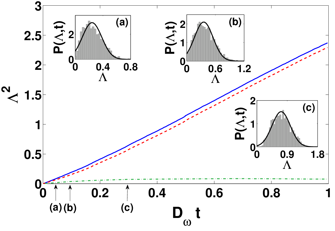
Having characterized the distribution by its and , we can now go back and deduce the expected values for the median and the average of . The median value is obtained by substitution of the prevalent squeezing parameter into Eq. (5),
| (9) |
whereas the mean value is found by averaging,
| (10) | |||||
As shown in Fig. 2, substitution of and from Fig. 4 into Eq. (9) and Eq. (10) gives excellent agreement with the median and true average of the distribution.
To conclude, small sampling errors of the normal distribution correspond to miss-sampling of the tail of the log-wide distribution of the spreading , whose median is distinct from its average. Since the average is strongly affected by the tails, we end up producing large errors. However, the miss-sampled tails can be properly deduced from a Gaussian approximation for the squeezing-parameter distribution, so as to overcome the sampling issue and get a prediction for the true average. We note that without performing this procedure, the average obtained by an experimentalist over many realizations of erratic driving is likely to reflect the median, which is the typical value, rather than the true average of the distribution.
VII Summary
We have studied the process of squeezing around the hyperbolic fixed point of the two site Bose-Hubbard model, in the presence of intense noise. We have greatly extended the quantitative understanding of the observed Quantum Zeno effect [13, 14] and investigated one of the principle paradigms in the theory of quantum noise, namely the replacement of an ideal quantum bath by deterministic erratic driving. We have shown that the interplay of diffusive quantum noise and hyperbolic squeezing results in log-wide statistical distributions of variances and fringe visibilities, so that their mean is different than their typical value. Consequently, we find that the fringe-visibility dynamics in a typical erratic driving scenario will differ from that obtained by coupling to an ideal quantum bath.
Acknowledgments.– We thank James Anglin for fruitful discussions. This research was supported by the Israel Science Foundation (grant Nos. 346/11 and 29/11) and by grant No. 2008141 from the United States-Israel Binational Science Foundation (BSF).
References
- [1] L. A. Khalfin, JETP Lett. 8, 65 (1968).
- [2] B. Misra and E. C. G. Sudarshan, J. Math. Phys. Sci. 18, 756 (1977).
- [3] Wayne M. Itano, D. J. Heinzen, J. J. Bollinger, and D. J. Wineland, Phys. Rev. A. 41, 2295 (1990).
- [4] S. Haroche and J.-M. Raimond, Exploring the Quantum: Atoms, Cavities, and Photons (Oxford, 2006).
- [5] A. G. Kofman and G. Kurizki, Nature (London) 405, 546 (2000).
- [6] A. G. Kofman and G. Kurizki, Phys. Rev. Lett. 87, 270405 (2001).
- [7] A. G. Kofman and G. Kurizki, Phys. Rev. Lett. 93, 130406 (2004).
- [8] G. Gordon and G. Kurizki, Phys. Rev. Lett. 97, 110503 (2006).
- [9] G. Gordon, N. Erez and G. Kurizki, J. Phys. B 40, S75 (2007).
- [10] A. M. Lane, Phys. Lett. 99A, 359 (1983).
- [11] A. G. Kofman and G. Kurizki, Phys. Rev. A 54, R3750 (1996).
- [12] P. Facchi and S. Pascazio, Prog. Phys. 49, 941 (2001).
- [13] Y. Khodorkovsky, G. Kurizki, and A. Vardi, Phys. Rev. Lett. 100, 220403 (2008); Phys. Rev. A 80, 023609 (2009).
- [14] C. Khripkov and A. Vardi, Phys. Rev. A 84, 021606(R) (2011).
- [15] C. M. Caves, Phys. Rev. D 23, 1693 (1981).
- [16] B. Yurke, S. L. McCall, and J. R. Klauder, Phys. Rev. A 33, 4033 (1986).
- [17] M. J. Holland and K. Burnett, Phys. Rev. Lett. 71, 1355 (1993).
- [18] M. Kitagawa and M. Ueda, Phys. Rev. A 47, 5138 (1993).
- [19] C. Gross, T. Zibold, E. Nicklas, J. Esteve, and M. K. Oberthaler, Nature 464, 7292 (2010).
- [20] M. F. Riedel, P. Böhi, Y. Li, T. W. Hänsch, A. Sinatra, and P. Treutlein, Nature bf 464, 1170 (2010).
- [21] R. Gati and M. Oberthaler, J. Phys. B 40, R61 (2007).
- [22] A. Vardi and J. R. Anglin, Phys. Rev. Lett. 86, 568 (2001); J. R. Anglin and A. Vardi, Phys. Rev. A 64, 013605 (2001);.
- [23] E. Boukobza, M. Chuchem, D. Cohen, and A. Vardi, Phys. Rev. Lett. 102, 180403 (2009).
- [24] Y. Castin and J. Dalibard, Phys. Rev. A 55, 4330 (1997).
- [25] M. Lewenstein and L. You, Phys. Rev. Lett. 77, 3489 (1996).
- [26] E. M. Wright, D. F. Walls and J. C. Garrison Phys. Rev. Lett. 77, 2158 (1996).
- [27] M. Javanainen and M. Wilkens, Phys. Rev. Lett. 78, 4675 (1997).
- [28] M. Greiner, M. O. Mandel, T. Hänsch, and I. Bloch Nature 419, 51 (2002).
- [29] A. Widera, S. Trotzky, P. Cheinet, S. Fölling, F. Gerbier, I. Bloch, V. Gritsev, M. D. Lukin, and E. Demler, Phys. Rev. Lett. 100, 140401 (2008).
- [30] M. Chuchem, K. Smith-Mannschott, M. Hiller, T. Kottos, A. Vardi, and D. Cohen, Phys. Rev. A 82, 053617(2010).
- [31] H. J. Lipkin, N. Meshkov, and A. J. Glick, Nucl. Phys. 62, 188 (1965); P.
- [32] Ribeiro, J. Vidal, and R. Mosseri, Phys. Rev. Lett. 99, 050402 (2007); P; Ribeiro, J. Vidal, and R. Mosseri, Phys. Rev. E 78, 021106 (2008).
- [33] R. Botet and R. Julien, Phys. Rev. B 28, 3955 (1983).
- [34] D. A. Garanin, X. Martines Hidalgo, and E. M. Chudnovsky, Phys. Rev. B 57, 13639 (1998).
- [35] In the numerical calculation, we discretize the time, dividing it into short steps of duration . The noise is realized by introducing a random rotation at the end of each step. This random walk process corresponds to erratic driving with the diffusion coefficient .