The elusive Heisenberg limit in quantum enhanced metrology

The typical quantum metrology scenario is as follows (see Fig. 1a). An ensemble of $N$ quantum systems undergo in parallel the same transformation $\Lambda_{\varphi}$, which depends on an unknown physical parameter $\varphi$. The output state is measured and the outcome is used to compute an estimate $\tilde{\varphi}$ of the parameter $\varphi$ as summarised below

The task is to find the optimal (possibly highly entangled) input state $\rho^{N}$ and the most effective measurement strategy in order to minimize the estimation error $\Delta\varphi_{N}$. Note that since the decoherence process is assumed to act independently on each of the probes, the global channel is described by the tensor product $\Lambda_{\varphi}^{\otimes N}$.

We pursue the estimation problem by restricting our attention to estimators which are unbiased in the neighbourhood of some fixed parameter value, for which the quantum Cramér-Rao bound holds

where $F_{Q}$ is the quantum Fisher information (QFI) [9]. Maximization of QFI over input states $\rho^{N}$ sets the limit on the achievable quantum enhanced precision:

The states that maximize the QFI and yield the HS for decoherence-free unitary channels are typically highly entangled: the GHZ state in the case of atomic spectroscopy [40], and the N00N state in the case of optical interferometry [41]. In the presence of decoherence, the optimal input states do not have an intuitive form and the maximization of the QFI (with rising $N$) becomes hard even numerically [30, 29, 20].

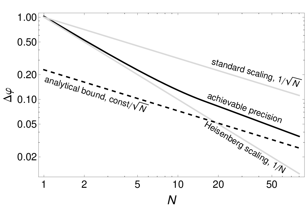
The typical behaviour of the estimation uncertainty in the presence of decoherence is depicted in the log-log scale in Fig. 2, showing that asymptotically in $N$ the quantum gain amounts to a constant factor improvement over the standard $1/\sqrt{N}$ scaling achievable with independent probes. The key result of this paper is to provide a method for a general and simple calculation of this constant factor improvement.

To understand the idea of CS, we need to think of quantum channels in a geometrical way [42]. A quantum channel is a completely positive, trace preserving map acting on density matrices. The space of all such transformations is convex: if $\Lambda,\Lambda^{\prime}$ are two channels, then $p\Lambda+(1-p)\Lambda^{\prime}$ can be realised by randomly applying $\Lambda$ or $\Lambda^{\prime}$ with probabilities $p$ and $1-p$. The channels that cannot be decomposed into a convex combination of different channels (e.g. the unitary transformations) are called extremal. Note that while all interior points of the space of quantum channels are non-extremal, the boundary contains both the extremal as well as some non-extremal channels.

We say that the family $\Lambda_{\varphi}$ is classically simulated [38] if each channel is written as a classical mixture of the form

where the unknown parameter enters only through the probability distribution $p_{\varphi}$ of a random variable $X$ that indicates which channel to pick from the set $\left\{\Lambda_{x}\!\right\}$ (see Fig. 1b). If $X_{1},\dots,X_{N}$ are independent hidden random variables used to generate the parallel channels we can rewrite the estimation problem as

Since conditionally on the values of $X_{i}$ the output state does not carry any information about $\phi$, the estimation precision in the above scenario is at most equal to that of the classical problem of estimating $\phi$ given $N$ independent samples from the distribution $p_{\phi}$

Hence, using the classical Cramér-Rao bound (CRB) [43] we obtain a lower bound on the uncertainty of the original problem (1)

where $F_{\textrm{cl}}$ is the classical Fisher information; see Methods for an alternative derivation.

Provided that $p_{\varphi}(x)$ satisfies regularity conditions required in the derivation of CRB [43], the SS of precision follows immediately. Moreover, any particular classical simulation yields an explicit SS bound on precision. If many CSs are possible, we obtain the tightest SS bound for $\Delta\varphi_{N}$ by choosing the “worst” decomposition yielding minimal $F_{\textrm{cl}}[p_{\varphi}]$, as shown below. On the other hand, HS is possible only when the above conditions are not satisfied. This happens in the decoherence-free case where $\Lambda_{\varphi}$ are unitary channels which are extremal points of the SQC and the only admissible $p_{\varphi}$ in (4) is the Dirac delta distribution being zero on all channels except $\Lambda_{\varphi}$. This yields $F_{\textrm{cl}}\!=\!\infty$, makes the bound trivial and leaves the possibility of HS, which is consistent with results of decoherence-free metrology.

The QFI at a given $\varphi_{0}$ depends only on the output state and its first derivative at $\varphi_{0}$. This implies that any family of channels $\tilde{\Lambda}_{\varphi}$ which “locally coincides” with the original one, i.e.

achieves the same maximum QFI in (3). It is therefore enough to consider the local classical simulations, i.e. any mixtures reproducing the channel and its first derivative at given $\varphi_{0}$. As proven in Supplementary Methods, Section I, the CS with the smallest $F_{\textrm{cl}}$ can be constructed using two channels, $\left\{\Lambda_{+},\Lambda_{-}\right\}$, that lie on the tangent line to the “channel trajectory” at the two outermost points situated on the boundary of the set of channels, see Fig 3. The local CS around $\phi_{0}$ reads explicitly

with

Making use of Eq. (5) applied to the binary probability distribution $p_{\varphi}^{\pm}$, we obtain

To calculate the above bound it suffices to find the “distances” $\varepsilon_{\pm}$ of the channel from the boundary measured along the tangent line. For extremal channels $\varepsilon_{\pm}=0$ and the bound is not useful. For non-extremal channels, the above construction will yield a finite $F_{\textrm{cl}}$ provided that $\varepsilon_{\pm}>0$, i.e. $\Lambda_{\varphi_{0}}$ can be decomposed into a mixture of channels lying on the tangent. Channels which have this additional property will be called $\varphi$-non-extremal. They obey the standard precision scaling, and include all full rank channels (i.e. channels lying in the interior of the SQC) [39, 38]. An explicit method for calculating $\varepsilon_{\pm}$ and hence the bound for a general quantum channel is described in the Methods section.

Even though the CS method is very general, there are interesting examples of $\varphi$-extremal decoherence models for which CS does not apply. In this case one can resort to the more powerful but less intuitive CE method.

The action of the quantum channel $\Lambda_{\varphi}$ can be described via its Kraus representation [44]:

with Kraus operators satisfying $\sum_{i}\!K_{i}(\varphi)^{\dagger}K_{i}(\varphi)\!=\!\openone$. Although this representation is not unique, different sets of linearly independent Kraus operators are related by unitary transformations

where $\mathbf{u}(\varphi)$ is a unitary matrix depending on $\varphi$.

An equivalent definition of the QFI has been proposed [39, 37]

where the minimization is performed over all $\varphi$ differentiable purifications of the output state

For pure input state, different purifications correspond to different equivalent Kraus representations of the channel, as in Eq. (8). For many quantum metrological models [37] one can make an educated guess of a purification and derive excellent input independent analytical bounds providing the correct asymptotic scaling of precision. Nevertheless, the method may be cumbersome especially when the channel description involves many Kraus operators.

A simpler bound can be derived by exploiting the intuitive observation that allowing the channel to act in a trivial way on an extended space, can only improve the precision of estimation, i.e.

This leads to an upper bound on $\mathcal{F}_{N}$, which goes around the input state optimization, yielding [39]:

where $\left\|\cdot\right\|$ denotes the operator norm, the minimization is performed over all equivalent Kraus representations of $\Lambda_{\varphi}$, and

where $\dot{\tilde{K}}_{i}(\varphi)\!=\!\partial_{\varphi}\tilde{K}_{i}(\varphi)$. For any given $\varphi=\varphi_{0}$, equation  (10) involves only $\tilde{K}_{i}$ and its first derivatives at $\varphi_{0}$. Moreover, the bound is insensitive to changing the Kraus representations with a $\varphi$ independent $\mathbf{u}$. Therefore, it is enough to parameterize equivalent Kraus representations in Eq. (8) with a hermitian matrix $\mathbf{h}$ which is generator of $\mathbf{u}(\varphi)=\exp[-\mathrm{i}\mathbf{h}(\varphi-\varphi_{0})]$. This reduces the optimization problem (10) to a minimization over $\mathbf{h}$.

Since the SS of precision holds when $\mathcal{F}_{N}$ scales linearly with $N$, the bound (10) implies that a sufficient condition for SS is to find $\mathbf{h}$ for which $\beta_{\tilde{K}}=0$, or equivalently[39]:

Here we go a step further and show that in this case we can obtain a quantitative SS bound

where the minimisation runs over $\mathbf{h}$ satisfying (12), and can be formulated as a semi-definite program, as described in the Methods section.

Moreover, it turns out that the bound resulting from finding the global minimum in Eq. (13) is at least as tight as the one derived using the CS method based on Eq. (5) (see Supplementary Methods, Section II) proving superiority of the CE over the CS method.

All examples of channels presented below are of the form $\Lambda_{\varphi}[\rho]\!=\!\Lambda\!\left[U_{\varphi}\rho U_{\varphi}^{\dagger}\right]$, i.e. a concatenation of a unitary rotation encoding the estimate parameter $\varphi$ and an $\varphi$-independent decoherence process. Consequently, $K_{i}(\varphi)\!=\!K_{i}U_{\varphi}$, where $K_{i}(\varphi)$, $K_{i}$ are the Kraus operators of $\Lambda_{\varphi}$ and $\Lambda$ respectively. The most relevant models in quantum enhanced metrology belong to this class, but the methods presented may be applied to more general models as well.

In what follows, we adopt the standard notation where $\openone$ is the $2\times 2$ identity matrix and $\left\{\sigma_{i}\right\}_{i=1}^{3}$ are the Pauli operators. We focus on two-level probe systems (qubits) sensing a phase shift modeled using a unitary $U\!(\varphi)=\exp[(\mathrm{i}\sigma_{3}\varphi)/2]$ — rotation of the Bloch ball around the $z$ axis. In the case of atomic clocks’ frequency calibration $\varphi\!=\!\delta\omega\!\cdot\!t$ with $\delta\omega$ being the detuning between the frequency of the atomic transition and the frequency of driving field, while $t$ the time of evolution. Even though in practice the parameter to be estimated is $\delta\omega$, we will consider that to be $\varphi$, in order to have a unified notation for atomic and optical models. In the case of a two mode optical interferometer, $U\!(\varphi)$ is the operator acting on a single photon state, accounting for the accumulated relative phase shift $\varphi$ between the two arms of the interferometer.

We apply the methods to four decoherence processes encountered in quantum enhanced metrology: two-level atom dephasing, depolarisation, spontaneous emission and the photon loss inside the interferometer. These examples will provide us with the full picture of the applicability of the methods discussed in the paper, as their cover all distinct cases from the point of view of the geometry of SQC.

Depolarization. Two level atom depolarization describes an isotropic loss of coherence and may be visualized by a uniform Bloch ball shrinking, see Fig. 4a, where $0\!\leq\!\eta\!<\!1$ is the final Bloch ball radius. Its description involves four Kraus operators

which makes it an example of a channel lying in the interior of the SQC. Using CS method we infer the SS of precision, and calculate the “distances” from the boundary of the SQC $\varepsilon_{\pm}\!=\!\sqrt{(1-\eta)(1+3\eta)}/(2\eta)$ (see Methods) resulting in the bound given in left column of Tab. 1a. Applying the CE method it is possible to further improve the bound and the result of the semi-definite optimization is shown in the right column of Tab. 1a. The only non zero elements of the corresponding optimal $\mathbf{h}$ are $\mathbf{h}_{03}=\mathbf{h}_{30}=\sqrt{(1-\eta)(1+3\eta)}/c$ and $\mathbf{h}_{12}=-\mathbf{h}_{21}=-\mathrm{i}(1+\eta)/c$ where $c=2(1-\eta)(1+2\eta)$. To our best knowledge, the bound has not been derived before.

Dephasing. Dephasing is a decoherence model of two-level atoms subject to fluctuating external magnetic/laser fields. In graphical representation, it corresponds to shrinking of the Bloch ball in $x,y$ directions with $z$ direction intact, see Fig. 4b. The canonical Kraus operators read [44]

where $0\!\leq\!\eta\!<\!1$ is the dephasing parameter. As it involves only two Kraus operators, it is not a full-rank channel and lies on the boundary of the SQC. It is, however, a non-extremal and more importantly non-$\varphi$-extremal channel allowing for the CS construction with $\varepsilon_{\pm}\!=\!\sqrt{1-\eta^{2}}/\eta$ (see Methods), yielding the bound given in Tab. 1b.

Most importantly, the above bound, is exactly the same as the one derived by Escher et al.[37] or by the CE method, where the minimum in Eq. (13) corresponds to $\mathbf{h}\!=\!\sigma_{1}/(2\sqrt{1-\eta^{2}})$. This proves that despite its simplicity the CS method may sometimes lead to bounds that are equally tight as the ones derived with much more advanced methods even for channels lying on the boundary of the SQC.

Spontaneous emission. The well known two-level atom spontaneous emission model is described by the Kraus operators

with $0\!\leq\!\eta\!<\!1$. Interestingly, for all $\eta$ this channel is extremal [45], which means that the CS is not applicable. Nevertheless, the CE method of Eq. (13), can be easily employed.

Substituting $K_{i}(\varphi)$ into Eq.(12) we find that the generator $\mathbf{h}$ is fixed to $\mathbf{h}=\frac{1}{2(1-\eta)}(\sigma_{z}-\eta\openone)$, Consequently, there is no need for minimization over $\mathbf{h}$ and from Eq. (13) we automatically obtain an SS bound listed in Tab. 1c which to our knowledge has not been reported in the literature before.

Lossy interferometer. In order to model loss in an optical interferometer, a third orthogonal state at the output, — vacuum — resulting from a loss of a photon, needs to be introduced. The decoherence channel on a single probe (single photon) is a map from a two to a three dimensional system:

where $\eta$ is the power transmission coefficient for the light traveling through each of the two arms. Although the corresponding channel $\Lambda_{\varphi}$ is non-extremal, it is unfortunately $\varphi$-extremal and CS cannot be used. Still, CE method can be easily applied. The optimal bound (see Tab. 1d) corresponds to $\mathbf{h}$ with non-zero elements $\mathbf{h}_{00}\!=-\mathbf{h}_{11}=\!\frac{1}{2(1-\eta)}$. This bound is asymptotically equally tight to the best bounds known in the literature [37, 35, 36] proving again that CE method despite its simplicity is able to provide powerful results in a straightforward manner.

In optical interferometric applications it is common to use states of light with an unbounded number of photons such as coherent or squeezed states. At a first glance it is not obvious that the model considered in the paper covers these situations. Formally speaking the bound we have derived applies to input states with a total number of photons fixed to $N$. Notice, however, that in every optical experiment what is measured in the end are photon numbers. If all phase reference beams are taken into account we can regard quantum states of light as incoherent mixtures of states occupying different total photon number sectors [46, 47]. From the point of view of metrology the QFI is then bounded from above by the weighted sum of QFIs for each of these sectors [30]. Within each sector we can easily apply our bound and since the bound is linear in $N$ the effective bound will simply correspond to replacing $N$ with $\bar{N}$ — mean number of photons in all relevant beams used in the experiment — and as such can be automatically applied to experiments involving coherent and squeezed light.

In order to demonstrate the practical relevance of the bound it is instructive to compare its predictions with the actual quantum enhancement observed recently in the GEO600 gravitational wave detector [17]. A detailed theoretical analysis of the setup from the perspective of the derived bounds is underway. Still, by reducing the essential features of the setup to a simple Mach-Zehnder interferometer, we can give a preliminary estimate on how far is the actual experiment from the optimal performance. For the reported overall optical transmission $\eta=0.62$ the theoretically predicted maximal quantum enhancement amounts to a $\sqrt{1-\eta}=0.62$ factor reduction in estimation uncertainty compared with the classical $1/\sqrt{\eta N}$ limit. The reported experimentally observed reduction was a factor of $0.67$ which is an indication that the experiment operates close to the fundamental quantum limit and any significant improvement is possible only if the optical loss is further reduced.

Assessing the impact of decoherence on the maximum possible quantum enhancement is a crucial element in developing quantum techniques for metrological applications. The tools developed in the paper allow for a direct calculation of bounds on the precision enhancement for arbitrary parameter estimation model where the decoherence process acts independently on each of the probes and may be represented with a finite number of Kraus operators. While the CE method is more powerful and for the most relevant metrological models yields in the asymptotic limit of large number of probes the tightest bounds known in the literature, the CS method may fail to provide equally tight bounds but provides an intuitive geometric insight into the absence of asymptotic HS in the presence of decoherence. From the derived bounds it is clear that if the HS was to be preserved for large number of probes $N$ the level of decoherence would have to decrease with increasing $N$ roughly as $(1-\eta)\approx 1/N$. This gives an estimate on the regime in which the quantum enhancement is quadratic as compared to the regime of constant factor improvement. This is clearly seen in Fig. 3 where this transition appears around $N\approx 1/(1-\eta)=20$ for $\eta=0.95$. Since in most metrology applications $N$ is larger by several order of magnitude, we expect that the SS scaling provides a reliable bound for the optimal estimation precision.

An important question that was not addressed in the paper is the saturability of the bounds. Clearly the CS method does not provide tight bounds in general as we have observed e.g. for depolarization channel. As to the CE method we are not able to prove that the bounds we have derived are saturable in the asymptotic limit. We should stress however, that these are lower bounds on estimation uncertainties and an upper bound can always be found by choosing a particular estimation method. Therefore if a particular strategy performs close to the derived bound, we can certify that it is near the fundamental quantum limit, as illustrated by the results of GEO600 experiment.

Note that even though the minimization over purification method[37] yields in principle a tight bound, in practice there is no effective algorithm to find a global minimum and the only way to convince oneself that the one has hit the global minimum is again to show that the theoretical lower bound on estimation uncertainty coincides with the performance of a particular estimation strategy.

The methods discussed were focused on deriving useful bounds in the asymptotic regime of large number of probes. Still, the bounds are valid (though weaker) for any value $N$. We leave it for a future work to improve the bounds for finite $N$ which seems to be possible by using the CE method and relaxing the $\beta_{\tilde{K}}=0$ constraint.

Proof of the classical simulation bound. In order to simplify the reasoning, let us focus on the classical simulations that are constructed using discrete sets of quantum channels, $\left\{\Lambda_{i}\right\}$. Then, the considered channel’s action of Eq. (4) can be rewritten as a $\varphi$-independent map acting on a larger input space [38]

where $\sigma_{\varphi}\!=\!\sum_{i}\,p_{\varphi,i}\left|e_{i}\right>\!\!\left<e_{i}\right|$ represents a diagonal state in a basis, in which $\Phi$ is defined via $\Phi[\varrho]\!=\!\sum_{i}\Lambda_{i}\!\otimes\!E_{i}\,[\varrho]$ with $E_{i}[\sigma]=\left<e_{i}\right|\sigma\left|e_{i}\right>$. In order to prove (5), we write the QFI for the $N$ parallel use of the channel and bound it from above, i.e.

exploiting the monotonicity of the QFI under any parameter independent quantum map[48], here $\Phi^{\otimes N}$.

Calculation of the classical simulation bound. The geometry of the space of channels and more specifically the $\varphi$-extremality are best viewed by using the Choi-Jamiołkowski isomorphism [49, 50]. Given a quantum channel $\Lambda\!:\mathcal{L}(\mathcal{H}_{\textrm{in}})\!\mapsto\!\mathcal{L}(\mathcal{H}_{\textrm{out}})$ acting from the space of density matrices on $\mathcal{H}_{\textrm{in}}$ to density matrices on $\mathcal{H}_{\textrm{out}}$, one defines $P_{\Lambda}\!=\!\Lambda\otimes\mathbb{I}\,[\left|\Phi\right>\!\left<\Phi\right|]$, where $\left|\Phi\right>\!=\!\sum_{i=1}^{\dim\mathcal{H}_{\textrm{in}}}|i\rangle\!\otimes\!|i\rangle$ is a maximally entangled state in $\mathcal{H}_{\textrm{in}}\otimes\mathcal{H}_{\textrm{in}}$. $\Lambda$ is a physical channel (i.e. trace preserving, completely positive map) iff $P_{\Lambda}$ is a positive semi-definite operator, satisfying $\textrm{Tr}_{\mathcal{H}_{\textrm{out}}}\!\{P_{\Lambda}\}\!=\!\openone$. If $\{K_{i}\}_{i}$ are the Kraus operators of the $\Lambda$ channel, we can write explicitly $P_{\Lambda}=\sum_{i}|K_{i}\rangle\langle K_{i}|$, where $|K_{i}\rangle=K_{i}\otimes\openone|\Phi\rangle$.

We can now say that, the channel $\Lambda_{\varphi}$ is not $\varphi$-extremal, if it is possible to find a non-zero $\varepsilon$, for which $P_{\Lambda_{\varphi}}\pm\varepsilon\,\partial_{\varphi}\!P_{\Lambda_{\varphi}}\geq 0$. See Supplementary Methods, Section III for an alternative formulation of the $\varphi$-extremality condition and its relation to the well known non-extremality condition due to Choi [50]. In practice, if we want to make most out of the bound in Eq. (7), we need to find the maximum values of $\varepsilon_{\pm}$, for which $P_{\Lambda_{\varphi}}\pm\varepsilon_{\pm}\,\partial_{\varphi}P_{\Lambda_{\varphi}}$ are still positive semi-definite operators. This is a simple eigenvalue problem and therefore the bound can be obtained immediately.

Taking the dephasing model as an example, the Choi-Jamiołkowski isomorphism of the corresponding $\Lambda_{\varphi}$ channel $P_{\Lambda_{\varphi}}\!=\!\sum_{i=1}^{2}|K_{i}U_{\varphi}\rangle\langle K_{i}U_{\varphi}|$ has a simple form:

It is easy to check that $P_{\Lambda_{\varphi}}\!\!+\!\varepsilon\,\partial_{\varphi}P_{\Lambda_{\varphi}}\!\geq\!0$ provided $|\varepsilon|\!\leq\!\sqrt{1-\eta^{2}}/\eta$, hence using Eq. (7) we arrive at the bound given in Table 1.

Channel extension method as a semi-definite program. Here we show that the minimization problem in Eq. (13) can be formulated as a simple semi-definite program. Let the channel $\Lambda_{\varphi}$ be a map from a $d_{1}$ to a $d_{2}$ dimensional Hilbert spaces with Kraus representation involving $k$ linear independent Kraus operators ($d_{2}\times d_{1}$ matrices). Consider the following block matrix:

where $\openone_{d}$ is a $d\times d$ identity matrix. Positive semi-definiteness of the matrix $A$ is equivalent to the condition

Minimizing the operator norm $\|\alpha_{\tilde{K}}\|$ is thus equivalent to minimizing $t$ subject to $A\geq 0$. Taking into account Eq. (12) the problem takes the form:

Since $\dot{\tilde{K}}_{i}=\dot{K}_{i}-\sum_{j}\mathrm{i}\mathbf{h}_{ij}K_{j}$ the matrix $A$ is linear in $\mathbf{h}$ and the problem is thus a semi-definite program with the resulting minimal $t$ being the minimal operator norm $\|\alpha_{\tilde{K}}\|$. For the purpose of this paper we have implemented the program using the CVX package for Matlab [51].

References

- [1] Giovannetti, V., Lloyd, S. & Maccone, L. Advances in quantum metrology. Nature Photon. 5, 222–229 (2011).
- [2] Maccone, L. & Giovannetti, V. Quantum metrology: Beauty and the noisy beast. Nature Phys. 7, 376–377 (2011).
- [3] Paris, M. G. A. Quantum estimation for quantum technology. Int. J. Quant. Inf. 7, 125–137 (2009).
- [4] Banaszek, K., Demkowicz-Dobrzanski, R. & Walmsley, I. A. Quantum states made to measure. Nature Photon. 3, 673–676 (2009).
- [5] Dirac, P. A. M. The Principles of Quantum Mechanics (Oxford University Press, 1958).
- [6] Kahn, J. & Guţă, M. Local Asymptotic Normality for Finite Dimensional Quantum Systems. Commun. Math. Phys. 289, 597–652 (2009).
- [7] Giovannetti, V., Lloyd, S. & Maccone, L. Quantum-enhanced measurements: beating the standard quantum limit. Science 306, 1330–1336 (2004).
- [8] Giovannetti, V., Lloyd, S. & Maccone, L. Quantum metrology. Phys. Rev. Lett. 96, 010401 (2006).
- [9] Braunstein, S. L. & Caves, C. M. Statistical distance and the geometry of quantum states. Phys. Rev. Lett. 72, 3439–3443 (1994).
- [10] Berry, D. W. & Wiseman, H. M. Optimal states and almost optimal adaptive measurements for quantum interferometry. Phys. Rev. Lett. 85, 5098–5101 (2000).
- [11] Zwierz, M., Pérez-Delgado, C. A. & Kok, P. General optimality of the heisenberg limit for quantum metrology. Phys. Rev. Lett. 105, 180402 (2010).
- [12] Mitchell, M. W., Lundeen, J. S. & Steinberg, A. M. Super-resolving phase measurements with a multi-photon entangled state. Nature 429, 161–164 (2004).
- [13] Eisenberg, H. S., Hodelin, J. F., Khoury, G. & Bouwmeester, D. Multiphoton path entanglement by nonlocal bunching. Phys. Rev. Lett. 94, 090502 (2005).
- [14] Nagata, T., Okamoto, R., O’Brien, J. L., Sasaki, K. & Takeuchi, S. Beating the standard quantum limit with four entangled photons. Science 316, 726–729 (2007).
- [15] Resch, K. J. et al. Time-reversal and super-resolving phase measurements. Phys. Rev. Lett. 98, 223601 (2007).
- [16] Higgins, B. L. et al. Demonstrating heisenberg-limited unambiguous phase estimation without adaptive measurements. New J. Phys. 11, 073023 (2009).
- [17] LIGO Collaboration. A gravitational wave observatory operating beyond the quantum shot-noise limit. Nature Phys. 7, 962–965 (2011).
- [18] Goda, K. et al. A quantum-enhanced prototype gravitational-wave detector. Nature Phys. 4, 472–476 (2008).
- [19] D. J. Wineland, W. M. I., J. J. Bollinger & Moore, F. L. Spin squeezing and reduced quantum noise in spectroscopy. Phys. Rev. A 46, R6797–R6800 (1992).
- [20] Huelga, S. F. et al. Improvement of frequency standards with quantum entanglement. Phys. Rev. Lett. 79, 3865–3868 (1997).
- [21] Meyer, V. et al. Experimental demonstration of entanglement-enhanced rotation angle estimation using trapped ions. Phys. Rev. Lett. 86, 5870–5873 (2001).
- [22] Leibfried, D. et al. Toward heisenberg-limited spectroscopy with multiparticle entangled states. Science 304, 1476–1478 (2004).
- [23] Wasilewski, W. et al. Quantum noise limited and entanglement-assisted magnetometry. Phys. Rev. Lett. 104, 133601 (2010).
- [24] Koschorreck, M., Napolitano, M., Dubost, B. & Mitchell, M. W. Sub-projection-noise sensitivity in broadband atomic magnetometry. Phys. Rev. Lett. 104, 093602 (2010).
- [25] Higgins, B. L., Berry, D. W., Bartlett, S. D., Wiseman, H. M. & Pryde, G. J. Entanglement-free heisenberg-limited phase estimation. Nature 450, 393–396 (2007).
- [26] Demkowicz-Dobrzanski, R, Multi-pass classical vs. quantum strategies in lossy phase estimation. Laser Phys. 20, 1197-1202 (2010).
- [27] Boixo, S, Flammia, S. T., Caves, S. T. & Geremia, J. M. Generalized Limits for Single-Parameter Quantum Estimation. Phys. Rev. Lett 98, 090401 (2007).
- [28] Napolitano, M., Koschorreck, M., Dubost, B., Behbood, M., Sewell, R. J. & Mitchell, M. W. Interaction-based quantum metrology showing scaling beyond the Heisenberg limit. Nature 471, 486–489 (2011).
- [29] Dorner, U. et al. Optimal quantum phase estimation. Phys. Rev. Lett. 102, 040403 (2009).
- [30] Demkowicz-Dobrzański, R. et al. Quantum phase estimation with lossy interferometers. Phys. Rev. A 80, 013825 (2009).
- [31] Shaji, A. & Caves, C. M. Qubit metrology and decoherence. Phys. Rev. A 76, 032111 (2007).
- [32] Andrè, A., S0rensen, A. S. & Lukin, M. D. Stability of atomic clocks based on entangled atoms. Phys. Rev. Lett. 92, 230801 (2004).
- [33] Meiser, D. & Holland, M. J. Robustness of heisenberg-limited interferometry with balanced fock states. New J. Phys. 11, 033002 (2009).
- [34] Kacprowicz, M., Demkowicz-Dobrzanski, R., Wasilewski, W., Banaszek, K. & Walmsley, I. A. Experimental quantum enhanced phase-estimation in the presence of loss. Nature Photon. 4, 357–360 (2010).
- [35] Kołodyński, J. & Demkowicz-Dobrzański, R. Phase estimation without a priori phase knowledge in the presence of loss. Phys, Rev. A 82, 053804 (2010).
- [36] Knysh, S., Smelyanskiy, V. N. & Durkin, G. A. Scaling laws for precision in quantum interferometry and the bifurcation landscape of the optimal state. Phys. Rev. A 83, 021804(R) (2011).
- [37] Escher, B. M., de Matos Filho, R. L. & Davidovich, L. General framework for estimating the ultimate precision limit in noisy quantum-enhanced metrology. Nature Phys. 7, 406–411 (2011).
- [38] Matsumoto, K. On metric of quantum channel spaces. arXiv 1006.0300v1 (2010).
- [39] Fujiwara, A. & Imai, H. A fibre bundle over manifolds of quantum channels and its application to quantum statistics. J. Phys. A: Math. Theor. 41, 255304 (2008).
- [40] Bollinger, J. J. ., Itano, W. M., Wineland, D. J. & Heinzen, D. J. Optimal frequency measurements with maximally correlated states. Phys. Rev. A 54, R4649–R4652 (1996).
- [41] Dowling, J. P. Correlated input-port, matter-wave interferometer: Quantum-noise limits to the atom-laser gyroscope. Phys, Rev. A 57, 4736–4746 (1998).
- [42] Bengtsson, I. & Zyczkowski, K. Geometry of quantum states: an introduction to quantum entanglement (Cambridge Univeristy Press, 2006).
- [43] Kay, S. M. Fundamentals of Statistical Signal Processing: Estimation Theory (Prentice Hall, 1993).
- [44] Nielsen, M. A. & Chuang, I. L. Quantum Computing and Quantum Information (Cambridge University Press, 2000).
- [45] Ruskai, M. B., Szarek, S. & Werner, E. An Analysis of Completely-Positive Trace-Preserving Maps on 2x2 Matrices. Lin. Alg. Appl. 347, 159–187 (2002).
- [46] Molmer, K. Optical coherence: A convenient fiction. Phys. Rev. A 55, 3195 (1996).
- [47] Jarzyna, M. & Demkowicz-Dobrzanski, R., Quantum interferometry with and without an external phase reference. Phys. Rev. A 85, 011801(R) (2012).
- [48] Fujiwara, A. Quantum channel identification problem. Phys. Rev. A 63, 042304 (2001).
- [49] Jamiolkowski, A. Linear transformations which preserve trace and positive semidefiniteness of operators. Rep. Math. Phys 3, 275–278 (1972).
- [50] Choi, M.-D. Completely positive linear maps on complex matrices. Lin. Algebr. Appl. 10, 285–290 (1975).
- [51] Grant M. & Boyd. S CVX: Matlab software for disciplined convex programming, http://cvxr.com/cvx/ (2011).