Radiation Transfer in the Cavity and Shell of Planetary Nebulae
Abstract
We develop an approximate analytical solution for the transfer of line-averaged radiation in the hydrogen recombination lines for the ionized cavity and molecular shell of a spherically symmetric planetary nebula. The scattering problem is treated as a perturbation, using a mean intensity derived from a scattering-free solution. The analytical function was fitted to H and H data from the planetary nebula NGC6537. The position of the maximum in the intensity profile produced consistent values for the radius of the cavity as a fraction of the radius of the dusty nebula: 0.21 for H and 0.20 for H. Recovered optical depths were broadly consistent with observed optical extinction in the nebula, but the range of fit parameters in this case is evidence for a clumpy distribution of dust.
Keywords:
stars: AGB and post-AGB – stars: evolution – Infrared: stars — (ISM:) planetary nebulae: general – ISM: jets and outflows – ISM: molecules –1 Introduction
Shells with internal cavities are found in almost all PNe [Balick & Frank 2002]. Such shells and cavities are related to the shaping of PNe by stellar winds. Low and intermediate mass stars lose their mass at a very high rate, forming a circumstellar envelope. Fast stellar winds from the central stars of PNe overtake the slower, denser, AGB ejecta, resulting in interaction of the fast and slow stellar wind components [Kwok, Purton & Fitzgerald 1978]. The fast wind sweeps the slow wind, and leaves a cavity inside. Cavities are also found in supernova remnants, [Dwek et al. 1987, Lagage et al. 1996] but these structures are more complicated [Bilikova et al. 2007]. Shell-cavity dimorphism is also found in LBV stars and in AGN.
In one of the well studied bipolar planetary nebulae, NGC 6537, the core consists of bright arcs tracing a shell surrounding an elongated cavity [Matsuura et al. 2005]. Arcs are bright in H and other recombination lines, and extinction maps derived from H and H suggests the presence of dust grains in the arcs. Matsuura et al. [Matsuura et al. 2005] suggested that little dust exists in the cavity. Deriving accurate dust density from H and H line maps is not straightforward, as the light from the central star is scattered within the arcs. In these arcs, both dust grains and gas are mixed together. Therefore, we developed a radiative transfer code to resolve cavity and shells for PNe, which includes scattered light in a shell.
A self-consistent radiative transfer code for this mixture has been developed by Ercolano, Barlow & Storey [Ercolano, Barlow & Storey 2005]. They have used a Monte Carlo method. Here, we use an analytical solution, with some approximations, and concentrate on the configuration of cavities and shells around them. The aim of the paper is therefore to obtain detailed physical insight through a simplified analytical model, which can complement the more complex information from numerical solutions.
2 The Model of NGC6537
In this section, we describe the physical and radiative transfer models that are used in our analysis of NGC 6573. Although certain parameters are definitely specific to this object, taken from Matsuura et al. [Matsuura et al. 2005], much of the model is generally applicable to any planetary nebula of similar geometry, and in a similar state of evolution.
2.1 Physical Model of the Nebula
We assume that the nebula NGC6537 is accurately spherically symmetric. The layout of the various radial zones of the object is summarised in Fig. 1. The central star is a white dwarf of negligible solid angle, both from an observer’s point of view, and from the modeller’s: no rays in the radiative transfer model are considered to start or end on the stellar surface.
The central star emits sufficient vacuum ultraviolet radiation to ionize a surrounding cavity. Ions in this cavity undergo frequent recombination and photoionization cycles, and it is the main source of H and H line radiation. For NGC6537 specifically, the observed flux ratio , where these fluxes are averages over the appropriate spectral-line bandwidth. From this ratio, we adopt radially constant values of the electron temperature, K, and electron number density, cm-3.
Surrounding the Hii cavity is a neutral shell, composed mainly of molecular material. This shell contains dust, which we assume, for the case of NGC6537, to have a mass fraction of . Most of the shell material is, of course, in the form of molecular hydrogen. The shell produces approximately two magnitudes of visual extinction in NGC6537, derived from the measured excess, . The shell is spatially resolved, and the extinction varies from magnitudes at the centre to magnitudes at off centre.
At present, we leave the form of the density profile as an unknown function in both the cavity and shell zones of the nebula.

2.2 Radiative Transfer Model
The volume element D in Fig. 1 has volume . If we let this be unit volume, then the radiated power per unit frequency and solid angle in the H line is
| (1) |
where is the ‘laboratory’ line-centre frequency of the H line, and is the Einstein coefficient for spontaneous emission. The subscripts refer to the principal quantum numbers of atomic hydrogen, so is the number density of H-atoms in the upper state of the transition. With an isothermal approximation, the lineshape function, is not a function of radius, but may be a function of direction if there are significant radial motions in the cavity or shell. Given these definitions, a similar expression may be written down for the emission coefficient of H:
| (2) |
We assume complete velocity redistribution, so that absorption lineshape functions are identical to those specified above for emission.
The radiative transfer equation is
| (3) | |||||
where is a unit vector along the ray of specific intensity . Opacity is provided by radius-dependent absorption coefficients, , , for the line and continuum, respectively, and the continuum scattering coefficient, . Kirchoff’s Law allows the continuum emission from dust to be written as , whilst the line emission coefficient is , and will be one of the specific forms in eq.(1) or eq.(2) for the appropriate transition. The final term on the right-hand side of eq.(3), equal to , is the scattering integral assuming isotropic, elastic scattering, and is the angle-averaged intensity.
We expand the left-hand side of eq.(3) in spherical polar coordinates (for example Peraiah [Peraiah 2002]). This introduces where is the angle between the direction of ray propagation and the radial direction. On the right, we combine the continuum absorption and scattering into an extinction coefficient, , and assume that the line absorption is negligible when compared to that in the continuum. The transfer equation with these modifications is
| (4) | |||||
We now integrate eq.(4) over the spectral-line bandwidth appropriate to either the H or the H line. We assume that this bandwidth is adequate to cover all the line radiation in the two hydrogen lines studied, regardless of all Doppler shifts within the source. In this connexion, we note that the velocity extent of the line due to the bulk motion of expansion is of order 20 km s-1, whilst the thermal Doppler width is 21.4 km s-1, with equal to the kinetic temperature in the ionized cavity in units of K. An unknown microturbulent width must be added in quadrature to the latter figure. It is therefore reasonable to suppose that even the extreme red- and blue-shifted portions of the line are significantly blended by the thermal and microturbulent lineshape. In other words, the combination of a low terminal expansion velocity and a large thermal plus microturbulent line width allows us to neglect velocity field induced Doppler shifts that would otherwise complicate the analysis considerably. Let the spectral-line bandwidth be , and the line-integrated intensity is given by
| (5) |
A similar equation to eq.(5) relates the angle-averaged intensities and . If we assume also that the functions , , and vary only very slightly over , these functions can be removed from the filter integral when it is applied to eq.(4). The result is
| (6) | |||||
where . The only frequency-dependent part of is the appropriate lineshape function (see eq.(1) and eq.(2)). We assume that the filter width is sufficient for the normalisation condition of the lineshape to hold, so that the integral in eq.(6) is either,
| (7) |
or the equivalent expression for H.
Finally, we re-write eq.(6) in separate forms appropriate to the cavity, and to the shell, respectively. In the cavity, we make the approximation that there is no dust, and that other processes, such as free-free and bound-free emission, make a negligible contribution to the radiation flux within the filter bandwidths used, for example Matsuura et al. [Matsuura et al. 2005]. The cavity therefore acts effectively as a pure source of line radiation, and the radiation transfer equation in this zone is,
| (8) |
By contrast, the shell, which is rich in dust, and where almost all the hydrogen is molecular, does not emit any H or H line radiation, is a site of continuum absorbtion, scattering and thermal emission by dust. The shell transfer equation is therefore,
| (9) | |||||
We now proceed to solve eq.(8) and eq.(9) in turn, coupling the solutions via boundary conditions. The solution is presented in several stages, and we outline these briefly here. In Section 3, we solve eq.(8) for the specific intensity of line radiation in the cavity, and this solution is angle-averaged in Section 4 yielding a mean intensity in the cavity as a function of radius. This quantity is not required for later calculations, so Section 4 is only included for completeness. In Section 5, we solve eq.(9) for radiative transfer in the shell: initially the specific intensity is obtained for dust extinction only, but a scattering source is then re-introduced as a perturbation. The cavity and shell solutions, for the specific intensity of a ray that may pass through both zones, are combined in Section 6. Section 7 is devoted to developing a mean intensity in the shell, as a function of radius, by angle-averaging the unperturbed solution from Section 6. This angle-averaged intensity is used to develop explicit forms for the scattering perturbation in Section 8. The remaining sections are concerned with observational properties of the solution, and fits to HST data for NGC6537.
3 The Cavity Solution

The layout of a typical ray passing through the cavity zone of the nebula is depicted in Fig. 2. The model cavity has no inner radius. All rays enter the cavity from the surrounding shell with some boundary value of the specific intensity. This value may differ from ray to ray, and, at present, we leave this value as an unknown. The emission coefficient depends on the radius only through the number density of H atoms in the upper level of the appropriate Balmer line from eq.(7). We make the approximation that these number densities are constants in the cavity, on the grounds that the cavity gas is in pressure equilibrium because of its high sound speed, and that we have already assumed a constant temperature in this region. We ignore the effect of overpressured regions near the edge of the cavity where the ionized medium is juxtaposed against the surrounding shell [Perinotto et al. 2004]. Therefore, we can re-cast eq.(8) as
| (10) |
where is the constant emission coefficient. The left-hand side of eq.(10) is the spherical polar expansion of the dot product, , but an alternative representation is as the derivative, , taken along the ray characteristic. An alternative way of writing eq.(10) is therefore,
| (11) |
which has the simple linear solution,
| (12) |
where is the unknown intensity with which the ray enters the cavity from the shell. The problem now consists only of re-expressing the distance along the characteristic, , in terms of the independent variables and . To obtain such a relation, we apply the sine rule to the triangle in Fig. 2, which is bounded by , and , yielding,
| (13) |
Now both and are constants, so it follows from the first equality in eq.(13) that
| (14) |
is a constant along the characteristic. Applying the cosine rule to the same triangle yields a quadratic equation in . The geometry of Fig. 2 requires the positive root, so that the distance along the characteristic is,
| (15) |
Using the result in eq.(14), and the definition of , we obtain . The constant expression under the square root reduces to , so the characteristic distance is . The intensity along the characteristic is therefore,
| (16) |
which is the required cavity solution for constant emission coefficient. It is trivial to prove, from eq.(16) that it satisfies eq.(10).
4 Mean Intensity in the Cavity
To obtain the angle-averaged intensity, , we need to integrate over a number of different rays, which all meet at one point, where the radius, , is a constant. At this point, is the final angle along its path, and can be used in the required solid angle integral. However, now is a variable, as we are integrating over many rays, and needs to be expressed in terms of , or . The situation is summarised in Fig. 3.

Results from the cavity solution, which still apply to Fig. 3, are that and . We use the first of these relations to eliminate from the second. The expression for can in turn be used to write the cavity solution, eq.(16) in the form,
| (17) |
noting that is the only variable on the right-hand side of eq.(17).
The solid angle integral for the mean intensity, with the integration over the azimuthal angle already carried out is
| (18) |
After substitution of eq.(17) into eq.(18), and a partial evaluation of the resulting integral, we find,
| (19) |
where , and is the angle average of . The result is a standard integral in terms of the arcsinh function, and after converting this to logarithmic form, the angle-averaged intensity is
| (20) |
We note that the apparent infinity in eq.(20) at disappears when this equation is replaced by a suitable expansion for the case . The small radius form is,
| (21) |
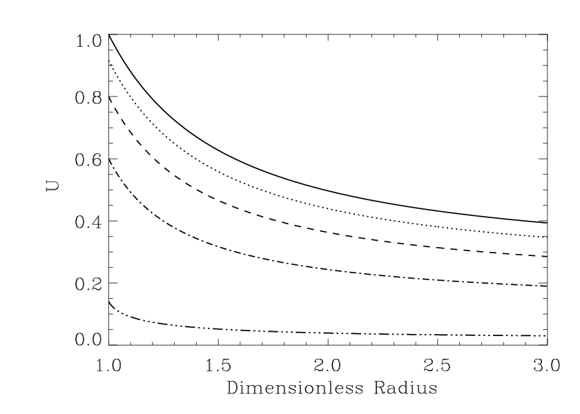
We plot, in Fig. 4, the function from eq.(20), as a function of the dimensionless radius .

5 The Shell Solution
We re-write the shell transfer equation as
| (22) |
where is an arbitrary function of the radius, which incorporates the continuum emission and line scattering. We change the left-hand side of eq.(22), as in the cavity solution, to describe a solution along the ray characteristic. The equation can then be put in standard first-order linear form as
| (23) |
Equation 23 may be integrated by the standard method of integrating factors. The boundary condition at is that the specific intensity enters the shell from interstellar space with the intensity , assumed equal to a typical value for Galactic starlight. The extinction coefficient at this same position is zero, regardless of its variation within the shell. With this condition imposed, eq.(23) has the formal solution,
| (24) | |||||
The ray distance, , is related to the radius and direction cosine by a modified form of the relation which appears in eq.(16). If the shell has an outer radius , then
| (25) |
where, for the moment, we ignore the presence of the cavity. With this same caveat, is a constant along a given ray if is the angle with which the ray enters the shell from interstellar space. Defining , we can express in terms of the radius as , which may be substituted into eq.(25) to yield a relation between and with no other variables involved. This relation, with the radius as the subject, is
| (26) |
The expression for the radius in eq.(26) can be used to expand the radius in terms of in eq.(24), provided that functional forms for and are known.
5.1 Shell Solution with Power-Law Density
To progress beyond eq.(24) we require some analytical approximation for the behaviour of the radius-dependent functions. We start with the extinction, . We assume that this depends on the radius only through the number density of the shell dust, so that the functional form is the same for both the absorption and scattering contributions. Further, we assume a density dependence which follows the inverse square behaviour of the singular isothermal sphere. Therefore, we suppose that the extinction in the shell behaves as
| (27) |
where is the maximum value of the extinction coefficient, found just outside the cavity boundary. With the help of eq.(26), we can write the extinction as a function of rather than . Integrals of the type which appear in eq.(24) can now be written in the form,
| (28) |
Introducing the new variables and , eq.(28) may be written as the standard integral,
| (29) |
which has the solution (as an indefinite integral),
| (30) |
Equation 24 contains two definite forms of eq.(30). The first of these has limits of to , and can be re-written, with the help of addition formulae for the arctangent from Gradshteyn & Ryzhik [Gradshteyn & Ryzhik 1965], as
| (31) |
where the is to be included only for ray distances such that , and the group . The second definite integral form from eq.(24) has the limits to , and it is convenient to write it without combining the arctangents, since the part with can be removed from the integral over . Overall, the shell solution can now be written,
| (32) | |||||
where
| (33) |
and the functional form of remains to be determined.
5.2 Scattering as a perturbation
If we ignore continuum emission in the shell, the unknown function, in eq.(32) reduces to line scattering alone, which depends on the angle-averaged mean intensity, . It is then possible, in principle, to average eq.(32) over solid angle, leading to an integro-differential equation for . However, owing to the difficulty in attempting to solve such an equation analytically, we resort to the simpler procedure of treating the scattering term as a perturbation. For this approximation to be very good, the scattering contribution to the extinction should be small, so that is a small parameter for all radii. This is unlikely to be true for real dust. For example, silicate dust modelled by Ossenkopf, Henning & Mathis [Ossenkopf, Henning & Mathis 1992] has an optical efficiency for scattering which is consistently 2-3 times that for absorption over optical wavelengths. However, we still adopt the perturbative approach as the only viable method of obtaining an approximate analytical solution. In this procedure, we first solve the radiative transfer equation in the shell, asuming that line extinction is the only contribution to the right-hand side of eq.(22). This means that we can set in eq.(32), and take as the zero-order solution in the shell,
| (34) | |||||
which is just the first term of eq.(32), with and eliminated in favour of , and with the help of the relation (see eq.(14), which still holds in the shell). It is tedious, but straightforward, to show that eq.(34) is indeed a solution of eq.(22), for the case where . Equation 34 cannot be used alone, as along any path through the nebula, a ray may encounter a sequence of shell, cavity, and again shell conditions. We therefore need to determine some functional form for for the case where a ray leaves the cavity and re-enters the shell, forming a combined solution along a ray.
As scattering is now to be treated as a perturbation, it can be computed from a mean intensity which is derived from the zeroth-order combined solution. An equation for a perturbation in the intensity, , can be constructed from eq.(9) by expanding the specific intensity as , and then subtracting off the equation in the zeroth-order estimate, . The result is,
| (35) |
where we have assumed that continuum emission makes a negligible contribution, so that . So, mathematically, the equation in the perturbation may be treated in the same way as the shell equation, eq.(22). The formal solution for therefore looks like eq.(24) with the scattering term replacing the unknown function . The perturbation solution is therefore given by
| (36) | |||||
where the function is given by eq.(30). It is important to note that there are three possible versions of eq.(36): A ray which avoids the cavity has and a lower limit of on the remaining integral. A ray which enters the cavity has two shell segments. In the first, and , but the upper limit is the value of the path where the ray enters the cavity. The perturbation is then constant in the cavity, forming a finite value of for the second shell segment, where is now the path length where the ray leaves the cavity.
6 The Combined Solution Along a Ray
Given the approximations made in the previous section, it is now possible to combine the cavity and shell solutions for a single ray. The geometry of the combined solution is set out in Fig. 5. As we are ignoring, as this stage, rays which pass solely through the shell, each effective ray has three segments: the first is an absorptive passage through the shell. However, if the input background at is very weak, we can ignore this segment, and treat the specific intensity of the ray at the cavity boundary, as zero.

The second segment of the ray path, between points Q and Q’ in Fig. 5, passes through the cavity. Here the specific intensity is assumed to increase through spontaneous emission in the line, according to the cavity solution, eq.(16). In particular, we want an expression for the specific intensity at Q’, where the cavity solution becomes the input value for the shell solution, which takes over as the third segment of the ray path, which continues until point Z is reached, and the ray passes into the vacuum.
At the point X in Fig. 5, which is as radius , the ray has travelled a distance through the shell, and it makes an angle with the radial vector. At this point, the solution will be the shell solution, with an input specific intensity from the cavity.
Analysis of the triangle MOQ shows that the cavity segment of the ray path has length . The total distance from point P to point M is, from the triangle MOP, equal to . Therefore, the ‘pre-cavity’ distance (from P to Q) is . The additional distance along the ray from M to X is . The total distance along the ray from P to X is therefore , just as in the shell solution, eq.(25). From these results, we find that the distance in Fig. 5 is given by
| (37) |
and by applying the sine rule to the triangle OPQ, the angles and are related by
| (38) |
which can be used to eliminate from eq.(37), yielding
| (39) |
The limiting (maximum) value of , for a ray which just enters the cavity, occurs when , when .
6.1 Input Solution to the Shell
As we are assuming that the specific intensity at point Q in Fig. 5 is effectively zero, the input solution for the shell is just the cavity solution evaluated at Q’. When this is done, the cavity solution, eq.(16) applies, with replacing . We take this solution with , and , obtaining . With the help of eq.(38), this expression becomes
| (40) |
which is the background for the solution in the shell beyond point Q’.
6.2 Combined Solution in the Shell
As the limits of integration are modified for the combined solution, we generate the shell solution from the indefinite integral, eq.(30). The upper limit is the distance along the ray path, , but the lower limit is now, from Fig. 5, . The result for the extinction integral is
| (41) | |||||
When eq.(25) has been applied, and eq.(41) has been re-expressed entirely in terms of , the result is,
| (42) | |||||
The first arctangent can be converted to a simpler form, as an arcsine, via the relation
| (43) |
which is taken from Gradshteyn & Ryzhik [Gradshteyn & Ryzhik 1965]. The second arctangent in eq.(42) can be written as the reciprocal of the form which appears in eq.(43) by defining the new variable . An additional relation linking arctangents [Gradshteyn & Ryzhik 1965] for the case where , which is true of , is
| (44) |
and this relation allows us to use eq.(43) directly on the second arctangent in eq.(42). A third relation from Gradshteyn & Ryzhik, allows us to re-write eq.(42) as,
| (45) |
It is now a simple matter to write out the combined solution for a ray by inserting eq.(45) into the shell solution, eq.(24), with given by eq.(40). With and fully expanded in terms of , the result is
| (46) | |||||
which is valid for . For plotting, we re-write eq.(46) in the form
| (47) |
an equation in two parameters, , and the optical depth parameter, . The latter parameter becomes equal to the radial optical depth of the shell in the limit where . The independent variable is . This last definition implicitly introduces a third parameter, the upper bound on , equal to . We note that eq.(47) reduces to a sensible limiting form, that is
| (48) |
for the case where . In Fig. 6 we show the function for five values of between its minimum value of zero, and maximum of 1. We set the optical depth parameter to be (see Section 10) to agree approximately with the visual extinction of magnitudes near the centre of NGC6537, and we plot the dimensionless radius out to .
7 Mean Intensity in the Shell
The approximation discussed in Section 6.1 - that rays that do not cross the cavity contribute zero specific intensity - excludes all rays with negative values of . Rays with non-zero specific intensity are limited to a subset of those with positive values of , more precisely to those with . With the additional restriction that any radius where is computed has , the situation here is similar to that shown in Fig. 3. The function to be averaged is the combined solution specific intensity in the zeroth-order (no scattering) approximation, given by eq.(46). The above considerations allow us to write a formal integral for the mean intensity, recalling that :
| (49) | |||||
We simplify eq.(49) via a series of substitutions. The first of these is to let the impact parameter be ; we also define the new constant parameters, , and . These definitions transform eq.(49) to,
| (50) | |||||
noting that and are always . Given this condition, we can expand the inverse sines in eq.(50) in terms of Gauss hypergeometric functions (for example, Abramowitz & Stegun [Abramowitz & Stegun 1965]). For complex argument ,
| (51) |
where the power series forming the Gauss hypergeometric function, , is absolutely convergent within, and on, the unit circle for the arguments in eq.(51) [Gradshteyn & Ryzhik 1965]. The substitution of eq.(51) into eq.(50) has the beneficial consequence of cancelling within the exponential, and leaving everywhere except for the product . This suggests the substitution , yielding,
| (52) | |||||
At this point, we expand the hypergeometric series which appear in eq.(52). For the case here, where the first two arguments are the same, the power series [Abramowitz & Stegun 1965] is
| (53) | |||||
in the case of general , , and for the specific case of and , we find,
| (54) |
Substitution of eq.(54) in eq.(52) leads to the expression
| (55) | |||||
which is as far as it is possible to proceed without making further approximations.
7.1 Approximate Forms
Although the series in eq.(55) is convergent for all relevant values of , convergence is rather slow when is close to , the condition for a ray in glancing contact with the cavity. However, the contribution of large to the integral is limited by the term in front of the exponential which tends to zero as (for the particular case of , see below). The physical reason for this is that rays at large angle have relatively short paths through the cavity, and correspondingly small specific intensities on entry to the shell.
Although values of which are close to (positions close to the shell/cavity boundary) can force the leading term in eq.(55) to , this is not a problem because, in this situation, the argument of the exponential approaches zero, the whole exponential to , and integration of the leading term alone is sufficient for moderate accuracy. We evaluate eq.(55) to two levels of accuracy in . In the zero-order approximation, we abandon all but the first term in the series, but this does not depend on , and can therefore be removed from the integral, leaving,
| (56) |
On evaluation of the integral in eq.(56), and reverting to the original radius variable, , we obtain the zero-order approximation to the mean intensity:
| (57) |
We note that at the cavity/shell boundary, where , the reduction of eq.(57) agrees with the cavity solution, eq.(20), evaluated at the same radius. Both equations yield .
It is also possible to obtain an analytic integral for a first order approximation, keeping the term in in the series in eq.(55). The integral in the first-order case is a standard form in Gradshteyn & Ryzhik [Gradshteyn & Ryzhik 1965]. With the parameters specific to the current problem, the integral is
| (58) | |||||
where . The first function, , on the right-hand side of eq.(58) is an Euler beta-function, whilst the second is a confluent hypergeometric series in two variables, and . Further standard formulae allow the beta-function to be expressed as a ratio of factorials that reduces to , so that the mean intensity to first order in is
| (59) |

We plot, in Fig. 7, the mean intensity in the shell as a function of dimensionless radius, , computed from the exact integral, eq.(50), and both approximations (eq.(57) and eq.(59)). For the value of the optical depth parameter used ( = 1.38, see Section 6.2), we see that even the zeroth-order formula is an excellent approximation. The graphs in Fig. 7 should be seen as an extension of that in Fig. 4 to values of and to in the case where the input background is negligible.
8 Perturbation Solution in the Shell
We now proceed to solve eq.(36) with the mean intensity in the scattering term given by eq.(57): it is too complicated to use the more accurate eq.(59). There are various forms of eq.(36) which should be used for the appropriate zone of the source. For a ray which penetrates the cavity, we initially consider the case where this ray has entered the shell, but has not yet reached the cavity. Assuming a negligible input intensity from the vacuum, we have the boundary condition that and , and therefore the problem for this ray, and zone, reduces to solving the integral,
| (60) |
The most useful form for the function , which appears in the integrating factor, for this zone is
| (61) |
which is derived from eq.(31), with a lower limit of and an upper limit of , followed by transformations similar to those used in working from eq.(43) to eq.(46). Note in particular that for a ray in this case, is an acute angle, but is obtuse, and the respective limits of these angles for a radial ray are zero and .
We substitute for the scattering coefficient, , by assuming that it has the same functional dependence as the absorption (see Section 5.1). The mean intensity is given by eq.(57). It is perfectly possible to express all these functions in terms of the distance, , along the ray, but the integral in eq.(60) appears easier when working in terms of radius. Letting the integral be , we have
| (62) | |||||
where as before, , , and the limits are given by
| (63) |
and
| (64) |
which reduces to for a ray entering the shell from the vacuum, and reaching the edge of the cavity, where . If we divide eq.(62) by the top line, which is independent of , we can carry out an integration by parts. The integrated part is
| (65) |
which removes the problematic square-root term. The result of this integration is,
| (66) | |||||
where the function , now entirely composed of logarithms and rational functions of , is defined by
| (67) |
and is given by
| (68) |
Note that the argument of the exponential in eq.(68) is different from that in eq.(62) because the original integral, that is the lower line of eq.(62), was multiplied by a factor of in order to obtain in eq.(66).
To calculate an approximation to the integral in eq.(66), we expand the argument of the exponential, noting that . The first term in the power-series expansion of the arcsine cancels with , and the next term is in which we ignore, such that
| (69) |
which is independent of , and can be moved outside the integral, which has now been reduced to the integration of the function from eq.(67). The integration of breaks down into six integrals, five of which can be solved in terms of elementary functions and the sixth in terms of the Riemann function [Gradshteyn & Ryzhik 1965]. A full form for the solution, , appears in Appendix A.
8.1 Rays which avoid the cavity
A ray which does not enter the cavity obeys the same propagation equation, eq.(60), but has a different upper limit on the distance, . Instead of integrating to the cavity boundary, we integrate to the mid-point, where the radial vector in perpendicular to the direction of the ray. At this point, the value of , and the corresponding radius is . We can therefore still use eq.(62), eq.(63) and eq.(64), but noting that the expression in eq.(64) now reduces to , rather than . The integrations and approximations which follow still apply, providing we use the new value of .
8.2 Outward bound rays
Provided that we are interested only in emergent rays, we can use the symmetry of the nebula to simplify matters greatly here. The integral along the ray, , is indentical, whether we are integrating inward to the midpoint (or cavity), or outward again towards the edge of the nebula. These integrals become formally the same because when we convert from to as the integration variable, we must use different roots of the expression
| (70) |
with the negative root required for the inward segment, and the positive root holding for the outward ray. The result is that the integrals over radius are identical. The form of eq.(60) which applies to outward rays is
| (71) |
where is now either the midpoint, for a ray which avoids the cavity, or the outward cavity boundary. We assume in eq.(71) that there is negligible scattering within the cavity. The input, , is just the inbound solution, evaluated at the midpoint or the inbound cavity boundary. If we define,
| (72) |
then we can re-write eq.(71) as
| (73) | |||||
noting that any constants in the exponentials have been cancelled between the term outside the integrals, and the inside. The equivalence of the integrals, , has been used, from the symmetry argument above. We can now write down two versions of eq.(73). The first is for a ray which avoids the cavity, where and on emerging from the cavity. In this case,
| (74) |
For the other case, where the ray crosses the cavity, the first value changes to ; the second remains the same, so we have,
| (75) |
where the integral is given in Appendix A (with appropriate limits).

In Fig. 8, we plot the emergent specific intensity for scattering, over the full range of entry angles to the nebula. The value of is the largest path length through the shell material for each angle. The same optical depth parameter for extinction, , has been used as in Fig. 6 and Fig. 7. The ratio of the outer (shell) radius to the inner (cavity) radius is : this has not been used as a formal parameter before, but the same value was also adopted for the above figures. The ratio of the scattering coefficient to the extinction coefficient has, rather arbitrarily, been set to . For the perturbative method to be accurate, this value should really be small, but is unlikely to be so for typical dust models (see discussion in Section 5.2). This parameter anyway acts as a simple scaling factor which does not change the shape of the function in Fig. 8. The normalising factor of is the same as in the other specific intensity plot, Fig. 6.
The marked cusp in the curve in Fig. 8 is at the expected angle, , where the ray switches from paths which enter the cavity to paths which do not. The path at this angle also corresponds to the maximum distance travelled through the shell material. The solution at smaller angles than that corresponding to the cusp comes from eq.(75); at larger angles, eq.(74) has been used.
9 Solution for Emergent rays
To use the symmetry property of the integral , we have already evaluated the perturbation, as an emergent quantity above. In general, the complete solution, for a given emergent ray, is given by,
| (76) |
where . For a ray which crosses the cavity, comes from a form of eq.(46) where and , whilst is given by eq.(75). Overall,
| (77) |
A ray which does not cross the cavity has only the contribution, and is given by eq.(74) without modification.
9.1 The observer’s view of the model
To an observer with perfect angular resolution, an emergent ray of given exit angle, , characterises a circular strip of a spherical surface. This strip has area , where is the polar angle measured from the line of sight towards the limb of the nebula. The observer cannot see this surface as a whole, but only a 2-D projection of it. The projected area of the strip is
| (78) |
It is straightforward to see that for any given strip, the polar angle is identical to the entry/exit angle of the ray, , which has allowed values between and . The observer with perfect angular resolution will therefore be able to pick out a small piece of a given (projected) strip, and will measure the associated specific intensity, , as a brightness. For a nebula of radius , at a distance from the observer, the measured brightness at an angle from the centre of the nebula, as seen by the observer, corresponds to exit angle . The brightness itself can be found by subsitituting this angle into either eq.(77) or eq.(74).
The other extreme observer’s view is that of a telescope with a beam that is much larger than the nebula. In this case, the specific intensity cannot be measured directly, and a flux, averaged over the whole object, is obtained instead. To a very good approximation, this flux is given by
| (79) |
where, as previously, the functional form of , is taken from eq.(77) or eq.(74), depending on whether or not the ray at angle traverses the cavity.
10 Fits to NGC6537
The function summarised in eq.(76) and eq.(77) was fitted to observational data describing the brightness variation of the H and H spectral lines as functions of angular position across the nebula. The fits were made with respect to four variable parameters in the theoretically-derived function: , the ratio of the cavity radius to the overall radius of the nebula; , the ratio of the scattering to extinction coefficients in the continuum; , the optical depth parameter, and an overall intensity-axis scale factor, , allowing a fit to normalized observational data. The optimum fit for each observational data set was taken to be that with the minimum value of the -statistic,
| (80) |
for a data set with entries of the form , and the four free parameters introduced above. Details of the treatment of the observational data, and of the fitting function, are described below.
10.1 Data from NGC6537
Data were extracted from Hubble Space Telescope H and H images [Matsuura et al. 2005]. Seven straight-line slices were taken through the nebula, each at a different angle on the sky. For each slice, data were recorded for both H and H, and for each slice and spectral line, data were organised into pairs consisting of a coordinate position along the slice, and a corresponding specific intensity. The following operations were applied to convert these data into a form suitable for fitting: For each slice and line, two pixel positions were found for the emission peaks, corresponding to the intersections of the slice with the cavity boundary. The coordinate origin was then shifted to the mid-point of the peak positions, and the absolute value of the slice coordinate taken, transforming the data to a pair of radial brightness profiles measured from an origin at the approximate centre of the nebula. An approximate correction for the aspherical nature of the nebula was imposed by re-scaling the radial axis such that the origin to peak distance was the same for all radial profiles. The outer radius of the nebula was taken to be the smallest maximum value on the new scale, and the remaining profiles truncated to the same distance. Finally, the new radial coordinate was re-scaled once more to the range , with corresponding to the now common outer radius. We note that the H data covered a larger angular range on average than the H data, leading to a larger value of in H by a factor of , and a different radial scaling for the two lines.
For individual radial profiles, the specific intensities were scaled such that the peak brightness was set to . Mean profiles for each spectral line were also constructed by averaging over all the un-normalized individual brightness profiles (on the normalised radial scale for each line defined above), and then normalising the averaged brightnesses to a peak height of .
In the averaged profiles, the standard errors resulting from the averaging process far exceeded the formal measurement errors in the observational data. The former were calculated at the peak position to be for H and for H, as fractions of the mean peak height. The latter were only of order and , respectively. For the normalised data sets, with peak heights of we assumed absolute uncertainties at all radial points to be equal to those at the respective peaks: for H and for H. The same absolute errors were assumed for the fits to the individual radial profiles. Values of were for H and for H.
10.2 Parameter ranges
The parameter has the formal range , but a much smaller realistic range can be selected for any radial profile by observing the position of the scattering peak (see also Fig. 8). Both the optical depth parameter, , and the scale-factor, , have the possible range . The most problematic parameter is , the ratio of the continuum scattering to extinction coefficients. The scattering has been treated as a perturbation in Section 8, so strictly speaking only the range is available to . However, from dust models, we expect the ratio of the scattering to absorption cross-sections to be of order (corresponding to ) in the optical region, as already discussed in Section 5.2. We have therefore fitted each profile twice: once for a true perturbation, with limited to the range , and once with the range , with the upper limit dictated by computed dust parameters. For each spectral line, we have fitted the averaged profile, and one selected individual profile. The fitting parameters for H and H have been taken to be entirely independent in this preliminary study.
10.3 Results of fitting
In Fig. 9 we show the results of the fits where the allowed range of is . The upper graphs are fits to H data, and the lower graphs, to H. For each line, the left-hand panels are fits to the averaged profile, whilst the right-hand panels show fits to a selected individual profile. Note that the individual H-fit (bottom right) is the only case in which the best fit fell in the perturbation range. A general difficulty with fits to averaged data is the broadening of the scattering peak in the averaging process, a consequence of the asphericity of the nebula that has only been approximately mitigated by the rescaling operations described in Section 10.1. A full table of the fitting parameters and quality estimates appears in Table 1.

| Line/Type | ||||||
|---|---|---|---|---|---|---|
| H/Avg | ||||||
| H/Avg | ||||||
| H/Ind | ||||||
| H/Ind | ||||||
| H/Avg | ||||||
| H/Avg | ||||||
| H/Ind |
Figure 10 shows the fits in which was restricted to the perturbation range, . Only in the case of the fit to the selected H profile was the best overall fit found in the perturbation range, and this fit has already been shown in Figure 9. We note that this particular fit has rather peculiar parameters (see Table 1), with a much larger optical depth parameter (and much smaller scattering parameter, ) than the others.

The easiest parameter to compare with observations is . Values of are markedly different for the two spectral lines, but this is simply a consequence of the greater angular extent of the data (larger ) for H. When corrected to the value of for H, by multiplying by , the values of for H, in the order they appear in Table 1, are and . These values are then consistent with those found for H. For the purposes of the optical-depth comparison (see below), it is useful to calculate uncorrected values of for both lines, yielding 0.79 for H and 0.87 for H.
We now consider the results for the optical depth parameter. In Section 2.1, the observed magnitude drops across the nebula, owing to extinction, ranged from 1.5 to 2.2 magnitudes, corresponding to intensity ratios of 0.251 and 0.132 along a line of sight. The respective optical depths are 1.38 and 2.03. We note that the fitted values of in Table 1 are of the optical depth parameter introduced at the end of Section 6.2, and that this is related to the optical depth of a radial ray passing through the full thickness of the nebula by (see eq.(48) with the limiting value of ). Fitted values of from the averaged data of 1.67 for H and 1.60 for H with the full range of then yield respective optical depths of 1.32 and 1.39. If the perturbation restriction is enforced, the optical depths are 1.90 and 1.74, results that are reasonably consistent with the observational values Note that considerably different optical depths are recovered from the selected individual profile, suggesting a locally clumpy medium.
11 Conclusion
An approximate analytical function has been derived that predicts the brightness of a spectral line, within some filter bandwidth, as a function of angular distance from the centre of a cavity/shell planetary nebula. The scattering part of this function is derived as a perturbation on the radiative transfer solution. This function has been fitted to observational data from NGC6537 in the H and H lines. The best-fit optical depth parameter in the model gives reasonable agreement with the observed optical extinction in the nebula. However, best-fit values for the scattering parameter are mostly too high to be consistent with a true perturbation. Consistent values were also found for the sizes of the cavity in both lines when the outer radius for H was applied to both spectral lines. The mean of the values of from Table 1 was , and the mean of the adjusted values for H was .
The analytical function may also have applications to other sources with a hot, largely ionized, interior, surrounded by a shell rich in dust. Examples include post-AGB stars, supernova remnants, symbiotic stars, quasars, and highly-magnetized planets in addition to the planetary nebulae discussed here.
ACKNOWLEDGMENTS
MDG acknowledges STFC (formerly PPARC) for financial support under the 2005-2010 rolling grant, number PP/C000250/1.
References
- [Abramowitz & Stegun 1965] Abramowitz M., Stegun I.M., 1965, Handbook of Mathematical Functions, Dover Publishing, New York, 8th Dover printing
- [Balick & Frank 2002] Balick B., Frank A., 2002, ARA&A, 40, 439
- [Bilikova et al. 2007] Bilikova J., Williams R.N.M., Chu Y.-H., Gruendl R.A., Lundgren B.F., 2007, AJ, 134, 2308
- [Dwek et al. 1987] Dwek E., Hauser M.G., Dinerstein H.L., Gillett F.C., Rice W.L., 1987, ApJ, 315, 571
- [Ercolano, Barlow & Storey 2005] Ercolano B., Barlow M.J., Storey P.J., 2005, MNRAS, 362, 1038
- [Gradshteyn & Ryzhik 1965] Gradshteyn I. S., Ryzhik I.M., 1965, Table of Integrals Series and Products, Academic Press, 4th edition.
- [Gray & Field 1995] Gray M. D., Field D., 1995, A&A, 298, 243
- [Kwok, Purton & Fitzgerald 1978] Kwok S., Purton C.R., Fitzgerald P.M., 1978, ApJ, 219, 125
- [Lagage et al. 1996] Lagage P.O., Claret A., Ballet J., Boulanger F., Cesarsky C.J., Cesarsky D., Fransson C., Pollock A., 1996, A&A, 315, 273
- [Matsuura et al. 2005] Matsuura M., Zijlstra A.A., Gray M.D., Molster F.J., Waters L.B.F.M., 2005, MNRAS, 363, 628
- [Ossenkopf, Henning & Mathis 1992] Ossenkopf V., Henning Th., Mathis J.S., 1992, A&A, 261, 567
- [Peraiah 2002] Peraiah A., 2002, An Introduction to Radiative Transfer, CUP, Cambridge
- [Perinotto et al. 2004] Perinotto M., Schönberner D., Steffen M., Calonaci C., 2004, A&A, 414, 993
Appendix A The Integral of
The solution shown here is for any ray. For a ray which enters the cavity, the upper limit of these integrals should be set to . For a ray which avoids the cavity, the upper limit should be . The integral of in eq.(67) breaks down into six integrals. The first two, trivially, are
| (81) |
and
| (82) |
The third can be integrated by parts, with the logarithm as the differentiated part. The result is,
| (83) | |||||
The fourth integral is the most problematic, as the result cannot be expressed in terms of elementary functions. If the integral is split, so that
| (84) | |||||
then both the expressions on the bottom line of eq.(84) conform to a standard integral [Gradshteyn & Ryzhik 1965], which is their no. 2.728 (version 2). The solution is written in terms of the function , which is discussed in detail in Section 9.55 of Gradshteyn & Ryzhik [Gradshteyn & Ryzhik 1965]. The final result is
| (85) | |||||
The fifth integral can be solved in a similar way to the simpler , integrating by parts with the logarithm as the differentiated part. The integrated part of the result can be solved by an expansion in partial fractions, and the overall expression is
| (86) | |||||
The final integral can be solved in a broadly similar manner to , and the solution is
| (87) | |||||