A Survey of Mg ii Absorption at with Magellan /
FIRE.
I: Sample and Evolution of the Mg ii Frequency
Alternate Affiliation: This paper includes data gathered
with the 6.5 meter Magellan Telescopes located at Las Campanas
Observatory, Chile
Abstract
We present initial results from the first systematic survey for Mg ii quasar absorption lines at . Using infrared spectra of 46 high-redshift quasars, we discovered 111 Mg ii systems over a path covering . Five systems have , with a maximum of —the most distant Mg ii system now known. The comoving Mg ii line density for weaker systems (Å) is statistically consistent with no evolution from to , while that for stronger systems increases three-fold until before declining again towards higher redshifts. The equivalent width distribution, which fits an exponential, reflects this evolution by flattening as before steepening again. The rise and fall of the strong absorbers suggests a connection to the star formation rate density, as though they trace galactic outflows or other byproducts of star formation. The weaker systems’ lack of evolution does not fit within this interpretation, but may be reproduced by extrapolating low redshift scaling relations between host galaxy luminosity and absorbing halo radius to earlier epochs. For the weak systems, luminosity-scaled models match the evolution better than similar models based on Mg ii occupation of evolving CDM halo masses, which greatly underpredict at early times unless the absorption efficiency of small haloes is significantly larger at early times. Taken together, these observations suggest that the general structure of Mg ii -bearing haloes was put into place early in the process of galaxy assembly. Except for a transient appearance of stronger systems near the peak epoch of cosmic star formation, the basic properties of Mg ii absorbers have evolved fairly little even as the (presumably) associated galaxy population grew substantially in stellar mass and half light radius.
Subject headings
Galaxies: evolution—Galaxies: halos—Galaxies: high-redshift—Infrared: general—intergalactic medium—quasars: absorption linesI. Introduction
Mg ii absorption line searches provide a luminosity-independent method for studying the distribution of gas in galactic haloes. While this technique has been employed for decades [70, 35, 66, 55, 64, 44, 50], using tens of thousands of sightlines [50, 51], these systematic surveys have all focused exclusively on Mg ii systems having . Only a handful of Mg ii absorption systems have been reported at redshifts based on serendipitous detections [16, 34, 28].
In this paper we present a systematic survey of intergalactic Mg ii absorption at using QSO spectra taken with FIRE (the Folded-port InfraRed Echellette) on the Magellan Baade Telescope. By characterizing the evolution of Mg ii absorption at higher redshifts we investigate the mechanisms which populate extended haloes with magnesium during the epoch when the cosmic SFR approached and passed its peak at .
Currently, two theories have been advocated to explain the properties of Mg ii absorbers at low redshifts. In one scenario, Mg ii traces cool clumps embedded in heated outflows from galaxies with high specific star formation rates. Alternatively, the distribution of Mg ii may reflect gravitational and gas accretion processes, as from dynamical mergers or cold accretion filaments.
The outflow hypothesis is supported by direct observations of blueshifted Mg ii absorption in the spectra of star forming galaxies [69]; Rubin et al. [54] have also observed this trend and established a correlation between Mg ii rest frame equivalent width and star formation rate (SFR). Moreover Bouché et al. [5] cross-correlated luminous red galaxies with 1806 Mg ii absorbing systems at from SDSS-DR3, finding an anti-correlation between Mg ii rest frame equivalent width and galaxy halo mass. This suggests that the individual Mg ii systems are not virialized, and the authors interpreted it as evidence that Mg ii systems trace star formation driven winds.
Concurrently, Zibetti et al. [74] showed with a sample of 2800 strong Mg ii absorbers () at low redshifts () that and galaxy color are correlated, with stronger Mg ii systems corresponding to the colors of blue star-forming galaxies. Follow up work [6, 40, 45, 43] supports this association of strong Mg ii systems with star forming galaxies.
Yet not all Mg ii absorbers are found around star forming galaxies. In particular, galaxy-selected Mg ii samples repeatedly show that star forming and early-type systems alike give rise to halo absorption, in proportions similar to the general field. Chen et al. [11] showed that the extent of the Mg ii halo increases with galaxy stellar mass but correlates only weakly with specific SFR for a sample of 47 weaker Mg ii (mostly with ) at . The authors interpreted this as evidence that the Mg ii absorbers reside in infalling clouds that eventually fuel star formation. In contrast to Zibetti, Chen et al. [10] see little correlation between strength and galaxy colors, a result corroborated by later research on weak absorbers [38, 30]. Kacprzak et al. [30] report a correlation between and galaxy inclination in a sample of 40 Mg ii absorption selected galaxies with and . This hints that some Mg ii absorbers may exhibit co-planar geometries and organized angular momenta, as may be found in accreting streams, satellites, and filaments, in contrast to star formation driven winds, which escape perpendicular to the disk.
The different interpretations of the above studies may be understood in terms of the selection processes used to construct each sample. Broadly speaking, galaxy surveys around QSO sightlines pre-selected for strong Mg ii absorption tend to find systems with high specific star formation rates [74, 6, 40, 45, 43]. Conversely, blind searches for Mg ii absorption along QSO sightlines serendipitously located near galaxies tend to find weaker Mg ii systems, and little correlation between Mg ii incidence and SFR [11, 10, 38].
Recently, the idea of a bimodal Mg ii absorber population has gained favor, with weaker absorbers mostly tracing distributed halo gas and stronger absorbers mostly tracing outflows [29]. This naturally explains the discrepant results between Mg ii-selected galaxies and galaxy-selected Mg ii absorbers: the two methods simply sample different ends of the Mg ii equivalent width distribution. While this explanation is simple and appealing, the existence of strong absorbers around fairly quiescent galaxies [24, 9, 23] suggests that in reality there may be significant overlap between the populations in space.
The volume-averaged SFR, halo assembly and cold accretion rates, and metal enrichment rate all vary with lookback time, but the restriction of for optical Mg ii searches means that these surveys do not sample epochs predating the SFR peak at . This inflection in the SFR density, along with the shutdown of cold accretion at low redshift, could be a useful diagnostic for evaluating the plausibility of the various mechanisms for distributing Mg ii into haloes.
While these factors motivate the study of Mg ii systems at high redshift, the endeavor has proven difficult in practice since the observed-frame transition moves into the near-infrared. In this regime, absorption line searches are hampered by blending with OH sky emission and telluric absorption, except at high resolutions where instrument sensitivity becomes an issue. We recently commissioned the FIRE infrared spectrometer on Magellan with the aim of studying C iv at ; its design characteristics also make it a powerful survey instrument for mapping Mg ii between and (and beyond as background targets are discovered). This paper describes the first results of an ongoing study of Mg ii absorption in early universe, based on an initial sample of 46 sightlines observed with FIRE.
In Section II we describe the data acquisition. In Section III we describe our analysis, including our Mg ii line identification procedure and completeness tests. In Section IV we provide our main science results, including binned and maximum likelihood fit population distributions, and compare these results to those of previous studies with lower redshift search ranges. In Section V, we discuss the implications of these results for the origin of Mg ii absorbing systems. Throughout this paper we use a CDM cosmology with , , and km s-1 Mpc-1.
II. Data Acquisition

Our sample consists of 46 quasar spectra taken with FIRE [59, 60], between 2010 June and 2011 April. This instrument is a single object, prism cross-dispersed infrared spectrometer with a spectral resolution of R=6000, or approximately 50 km/s, over the range 0.8 to 2.5 m. We observed using a 0.6” slit and with a typical seeing of 0.5”-0.8”. The wavelength coverage of FIRE set the lower redshift limit for our Mg ii absorption doublet search at in each sightline. The QSO emission redshifts, which ranged from to , typically set the upper limits (although masked telluric regions described below sometimes decreased these maximum cutoffs). Regions lying within km s-1 of each background QSO were excluded from the search path, although the effect of this cut was negligible on our derived results. Table 1 lists key observational properties of the 46 quasars. The quasars themselves were predominantly chosen from the SDSS DR7 quasar catalog [57], with an additional, somewhat heterogeneous selection of bright, well known objects from the literature.
| Object | SNRaaMedian signal-to-noise ratio per pixel across Mg ii pathlength. | |||
|---|---|---|---|---|
| Q0000-26 | 4.10 | 1.95-3.83 | 1226 | 20.7 |
| BR0004-6224 | 4.51 | 1.95-4.51 | 1764 | 8.2 |
| BR0016-3544 | 4.15 | 1.95-3.83 | 2409 | 14.0 |
| SDSS0106+0048 | 4.45 | 1.95-4.45 | 3635 | 18.9 |
| SDSS0113-0935 | 3.67 | 1.95-3.67 | 1944 | 12.8 |
| SDSS0127-0045 | 4.08 | 1.95-3.83 | 3635 | 22.5 |
| SDSS0140-0839 | 3.71 | 1.95-3.71 | 1226 | 18.2 |
| SDSS0203+0012 | 5.85 | 1.98-5.40 | 3635 | 4.0 |
| SDSS0244-0816 | 4.07 | 1.95-3.83 | 1944 | 12.9 |
| BR0305-4957 | 4.78 | 1.95-4.78 | 2409 | 28.2 |
| BR0322-2928 | 4.62 | 1.95-4.62 | 2409 | 21.1 |
| BR0331-1622 | 4.32 | 1.95-4.32 | 1944 | 15.1 |
| SDSS0331-0741 | 4.74 | 1.95-4.74 | 2177 | 6.2 |
| SDSS0332-0654 | 3.69 | 1.95-3.69 | 2409 | 5.6 |
| SDSS0344-0653 | 3.96 | 1.95-3.83 | 3022 | 6.6 |
| BR0353-3820 | 4.58 | 1.95-4.58 | 1200 | 26.7 |
| BR0418-5723 | 4.37 | 1.95-4.37 | 4200 | 8.5 |
| SDSS0818+1722 | 5.90 | 2.00-5.40 | 9000 | 10.2 |
| SDSS0836+0054 | 5.82 | 1.96-5.40 | 10187 | 15.8 |
| SDSS0842+0637 | 3.66 | 1.95-3.66 | 2409 | 9.1 |
| SDSS0935+0022 | 5.82 | 1.96-5.40 | 1817 | 11.1 |
| SDSS0949+0335 | 4.05 | 1.95-3.83 | 1817 | 13.6 |
| SDSS1020+0922 | 3.64 | 1.95-3.64 | 2409 | 15.2 |
| SDSS1030+0524 | 6.28 | 2.16-6.28 | 14400 | 5.0 |
| SDSS1037+0704 | 4.10 | 1.95-3.83 | 2726 | 8.1 |
| SDSS1110+0244 | 4.12 | 1.95-3.83 | 2409 | 18.6 |
| SDSS1135+0842 | 3.83 | 1.95-3.83 | 2409 | 17.7 |
| SDSS1249-0159 | 3.64 | 1.95-3.64 | 1817 | 18.2 |
| SDSS1305+0521 | 4.09 | 1.95-3.83 | 1363 | 8.8 |
| SDSS1306+0356 | 5.99 | 2.04-5.99 | 15682 | 6.4 |
| ULAS1319+0950 | 6.13 | 2.10-6.13 | 19275 | 5.0 |
| SDSS1402+0146 | 4.16 | 1.95-3.83 | 1902 | 15.0 |
| SDSS1408+0205 | 4.01 | 1.95-3.83 | 2409 | 9.9 |
| SDSS1411+1217 | 5.93 | 2.01-5.93 | 3600 | 8.6 |
| Q1422+2309 | 3.65 | 1.95-3.65 | 1226 | 47.2 |
| SDSS1433+0227 | 4.72 | 1.95-4.72 | 2409 | 13.4 |
| CFQS1509-1749 | 6.12 | 2.10-6.12 | 9900 | 9.7 |
| SDSS1538+0855 | 3.55 | 1.95-3.55 | 1363 | 24.2 |
| SDSS1616+0501 | 4.87 | 1.95-4.87 | 1800 | 5.2 |
| SDSS1620+0020 | 4.09 | 1.95-3.83 | 972 | 7.0 |
| SDSS1621-0042 | 3.70 | 1.95-3.70 | 1204 | 26.1 |
| SDSS2147-0838 | 4.59 | 1.95-4.59 | 2409 | 13.8 |
| SDSS2225-0014 | 4.89 | 1.95-4.89 | 7200 | 11.5 |
| SDSS2228-0757 | 5.14 | 1.95-5.14 | 3600 | 4.9 |
| SDSS2310+1855 | 6.04 | 2.06-6.04 | 14400 | 17.5 |
| BR2346-3729 | 4.21 | 1.95-3.83 | 2409 | 11.0 |
We reduced the data using a custom-developed IDL pipeline named FIREHOSE, which has been released to the community as part of the FIRE instrument package. This pipeline evolved from the optical echelle reduction software package MASE [4]. FIREHOSE contains many important modifications for IR spectroscopy, including using terrestrial OH lines imprinted on science spectra for wavelength calibration.
To correct for telluric absorption features, we obtained spectra of A0V stars at comparable observing times, airmasses and sky positions to our observed QSOs. We then performed telluric corrections and relative flux calibrations using the xtellcor software package released with the spextool pipeline [13], which employs the method of Vacca et al. [67]. Regions lying between the and bands (1.35 m to 1.48 m, excluding 3.8 to 4.3 for Mg ii systems) and the and bands (1.79 m to 1.93 m, excluding 5.4 to 5.9), were masked out of the search path. Another smaller region of path length centered on (near the - transition) showed poor telluric residuals (noticeable in Figure 1). We left this region in our Mg ii search since it was still possible to find strong systems (we found six). We report these systems in our line lists but exclude this path and associated systems from our population statistics as the sample completeness is low and variable from one sightline to the next.

The final signal-to-noise ratios per pixel for our full QSO set ranged from 4.0 to 47.2, with a median value of 12.9. Figure 1 shows the Mg ii search portions for our highest (top panel), a typical (middle panel), and a relatively poor (bottom panel) signal-to-noise spectra.
III. Analysis
III.1. Mg ii Line Identification
III.1.1 Continuum Fitting
With just 46 QSO sightlines in our sample, it would be reasonable to fit each continuum manually. However, as part of our downstream analysis we also run extensive Monte Carlo tests to characterize sample completeness. We wished to capture the effects of the continuum fitting on our completeness. Accordingly, we developed an automated algorithm for continuum fitting, to make treatment of the Monte Carlo sample both tractable, and as consistent as possible with our handling of the true data.
First, we generated an initial line mask to prevent absorption and emission features (including miscorrected skylines) from biasing the continuum. Next, we performed iterative, sigma-clipped linear fits on the masked data over small segments of the spectra (100 pixels, or 1250 km/s, wide) in order to determine a list of spline knots (with two knots drawn from each of these small segments). We then implemented a cubic spline fit through these knots to produce a continuum fit. Since knowledge of the continuum fit facilitates the creation of the initial line mask, we iterated this between two and five times before converging on a final continuum fit.
III.1.2 Matched Filter Search
After obtaining continuum-normalized spectra, we ran a matched filter search with a signal-to-noise ratio cut of 5 to determine an initial candidate list. The filter kernel consists of a pair of Gaussian profiles separated by the Mg ii spacing with FWHM ranging from 37.5 to 150 km/s. Sky subtraction residuals near OH lines are a source a noise in the infrared, so we identified and masked badly miscorrected sky lines before running this convolution to reduce the number of false positives. Even with this masking, this matched filter search typically led to 50 to 100 candidates per QSO sightline, of which only per sightline were true detections.
To mitigate the high false positive rate of the matched filter procedure, we fit each candidate doublet with a pair of Gaussian absorption profiles and subjected the resulting fit parameters to a set of consistency checks (e.g. within errors). This additional doublet fitting filter step reduced the number of false positives by a factor of 10, and left us with 256 candidates across all QSO sightlines.
III.1.3 Visual Inspection
We subjected these machine generated candidates to a visual inspection to produce the final Mg ii sample list. This interactive step lowered the final list to 110 Mg ii systems (plus one proximate system). Despite our best efforts to automate the process, we found that the poorly telluric corrected regions and abundance of sky lines mandated this visual inspection.
We also visually combed through all 46 spectra to identify systems missed by the automated line finder. We found three systems with this visual search that our automated line finding algorithm rejected. One system was a large 2.62Å system that was “too complex” (and therefore was fit poorly by a Gaussian absorption profile and consequently rejected), and the other two were smaller systems (confirmed by FeII lines) that were partially obscured by sky lines. The two smaller systems were manually added to our line list in Table 2, but were not included in statistical calculations so as not to bias our results by counting them and then overcorrecting for completeness. The large system’s equivalent width was greater than the highest value () probed in our Monte Carlo completeness tests. We are complete to such large systems, so this system was included in our statistical calculations.
III.1.4 Final Mg ii Sample

| Index # | Sightline | ||||||
|---|---|---|---|---|---|---|---|
| (Å) | (Å) | (Å) | (Å) | (km s-1) | |||
| 1 | Q0000-26 | 2.184 | 0.162 | 0.031 | 0.112 | 0.026 | 166.0 |
| 2 | Q0000-26 | 3.390 | 1.356 | 0.016 | 1.145 | 0.016 | 259.7 |
| 3 | BR0004-6224 | 2.663 | 0.260 | 0.045 | 0.140 | 0.036 | 58.0 |
| 4 | BR0004-6224 | 2.908 | 0.596 | 0.047 | 0.183 | 0.028 | 83.3 |
| 5 | BR0004-6224 | 2.959 | 0.569 | 0.063 | 0.669 | 0.047 | 108.4 |
| 6 | BR0004-6224 | 3.203 | 0.558 | 0.029 | 0.548 | 0.026 | 86.8 |
| 7 | BR0004-6224 | 3.694 | 0.236 | 0.042 | 0.234 | 0.019 | 79.6 |
| 8 | BR0004-6224 | 3.776 | 1.045 | 0.046 | 1.049 | 0.043 | 169.7 |
| 9 | BR0016-3544 | 2.783 | 0.517 | 0.027 | 0.305 | 0.026 | 101.2 |
| 10 | BR0016-3544 | 2.819 | 4.028 | 0.050 | 3.639 | 0.053 | 605.5 |
| 11 | BR0016-3544 | 2.949 | 0.157 | 0.026 | 0.144 | 0.035 | 79.6 |
| 12 | BR0016-3544 | 3.757 | 1.559 | 0.041 | 1.430 | 0.050 | 551.4 |
| 13 | SDSS0106+0048 | 3.729 | 0.842 | 0.016 | 0.673 | 0.015 | 194.9 |
| 14 | SDSS0113-0935 | 2.825 | 0.194 | 0.029 | 0.110 | 0.029 | 94.0 |
| 15 | SDSS0113-0935 | 3.544 | 0.228 | 0.037 | 0.186 | 0.035 | 133.6 |
| 16 | SDSS0113-0935 | 3.617 | 0.563 | 0.024 | 0.344 | 0.020 | 155.3 |
| 17 | SDSS0127-0045 | 2.588 | 1.602 | 0.025 | 1.164 | 0.025 | 457.8 |
| 18 | SDSS0127-0045 | 2.945 | 2.253 | 0.038 | 1.583 | 0.037 | 529.7 |
| 19 | SDSS0127-0045 | 3.168 | 0.309 | 0.024 | 0.138 | 0.016 | 198.5 |
| 20 | SDSS0127-0045 | 3.728 | 0.824 | 0.012 | 0.745 | 0.012 | 176.9 |
| 21 | SDSS0140-0839 | 2.241 | 0.405 | 0.031 | 0.686 | 0.043 | 144.4 |
| 22aaPoor telluric region | SDSS0140-0839 | 3.081 | 0.558 | 0.018 | 0.410 | 0.027 | 126.4 |
| 23 | SDSS0140-0839 | 3.212 | 0.081 | 0.014 | 0.092 | 0.014 | 126.4 |
| 24bbProximate system | SDSS0140-0839 | 3.697 | 0.604 | 0.014 | 0.308 | 0.009 | 173.3 |
| 25 | SDSS0203+0012 | 3.711 | 0.374 | 0.038 | 0.250 | 0.065 | 122.8 |
| 26aaPoor telluric region | SDSS0203+0012 | 4.313 | 0.849 | 0.093 | 0.824 | 0.080 | 198.5 |
| 27 | SDSS0203+0012 | 4.482 | 0.670 | 0.183 | 0.623 | 0.024 | 126.5 |
| 28 | SDSS0203+0012 | 4.978 | 0.886 | 0.039 | 0.791 | 0.056 | 151.6 |
| 29 | BR0305-4957 | 2.502 | 0.331 | 0.024 | 0.169 | 0.022 | 137.2 |
| 30 | BR0305-4957 | 2.629 | 1.113 | 0.018 | 0.959 | 0.023 | 220.1 |
| 31 | BR0305-4957 | 3.354 | 0.564 | 0.013 | 0.412 | 0.012 | 144.5 |
| 32 | BR0305-4957 | 3.591 | 1.373 | 0.017 | 1.207 | 0.013 | 306.5 |
| 33 | BR0305-4957 | 4.466 | 1.792 | 0.017 | 1.478 | 0.029 | 302.9 |
| 34 | BR0322-2928 | 2.229 | 0.618 | 0.020 | 0.510 | 0.021 | 112.1 |
| 35 | BR0331-1622 | 2.295 | 1.836 | 0.067 | 1.714 | 0.056 | 403.8 |
| 36 | BR0331-1622 | 2.593 | 0.223 | 0.019 | 0.185 | 0.019 | 76.0 |
| 37 | BR0331-1622 | 2.927 | 1.382 | 0.039 | 1.098 | 0.045 | 346.1 |
| 38 | BR0331-1622 | 3.557 | 0.707 | 0.033 | 0.582 | 0.033 | 130.0 |
| 39aaPoor telluric region | SDSS0332-0654 | 3.061 | 0.883 | 0.084 | 0.608 | 0.059 | 162.4 |
| 40 | BR0353-3820 | 1.987 | 3.131 | 0.030 | 2.717 | 0.026 | 508.2 |
| 41 | BR0353-3820 | 2.696 | 0.381 | 0.014 | 0.232 | 0.014 | 187.7 |
| 42 | BR0353-3820 | 2.754 | 4.599 | 0.016 | 4.325 | 0.019 | 616.3 |
| 43 | BR0418-5723 | 2.030 | 1.449 | 0.072 | 1.009 | 0.080 | 209.3 |
| 44aaPoor telluric region | BR0418-5723 | 2.978 | 1.850 | 0.072 | 2.136 | 0.099 | 263.3 |
| 45 | SDSS0818+1722 | 3.563 | 0.640 | 0.072 | 0.427 | 0.029 | 151.7 |
| 46 | SDSS0818+1722 | 4.431 | 0.457 | 0.052 | 0.138 | 0.010 | 108.4 |
| 47 | SDSS0818+1722 | 5.065 | 0.841 | 0.061 | 0.533 | 0.046 | 151.7 |
| 48 | SDSS0836+0054 | 2.299 | 0.455 | 0.022 | 0.300 | 0.021 | 130.0 |
| 49 | SDSS0836+0054 | 3.744 | 2.607 | 0.024 | 1.992 | 0.031 | 443.4 |
| 50 | SDSS0949+0335 | 2.289 | 2.852 | 0.062 | 2.408 | 0.054 | 421.8 |
| 51 | SDSS0949+0335 | 3.310 | 2.033 | 0.039 | 1.665 | 0.033 | 339.0 |
| 52 | SDSS1020+0922 | 2.046 | 0.406 | 0.045 | 0.288 | 0.047 | 112.0 |
| 53 | SDSS1020+0922 | 2.593 | 0.464 | 0.026 | 0.499 | 0.022 | 144.5 |
| 54 | SDSS1020+0922 | 2.749 | 0.652 | 0.023 | 0.518 | 0.024 | 151.7 |
| 55 | SDSS1020+0922 | 3.479 | 0.118 | 0.016 | 0.085 | 0.019 | 104.8 |
| 56 | SDSS1030+0524 | 2.188 | 0.317 | 0.017 | 0.291 | 0.017 | 133.7 |
| 57ccMissed by automated search algorithm | SDSS1030+0524 | 2.780 | 2.617 | 0.069 | 1.855 | 0.086 | 583.9 |
| 58 | SDSS1030+0524 | 4.583 | 1.857 | 0.031 | 2.139 | 0.127 | 367.7 |
| 59 | SDSS1030+0524 | 4.948 | 0.447 | 0.017 | 0.278 | 0.019 | 162.4 |
| 60 | SDSS1030+0524 | 5.130 | 0.138 | 0.013 | 0.089 | 0.023 | 76.0 |
| Index # | Sightline | ||||||
|---|---|---|---|---|---|---|---|
| (Å) | (Å) | (Å) | (Å) | (km s-1) | |||
| 61 | SDSS1110+0244 | 2.119 | 3.041 | 0.041 | 2.884 | 0.042 | 454.2 |
| 62 | SDSS1110+0244 | 2.223 | 0.205 | 0.024 | 0.121 | 0.029 | 166.0 |
| 63 | SDSS1305+0521 | 2.302 | 1.993 | 0.095 | 1.533 | 0.095 | 234.5 |
| 64 | SDSS1305+0521 | 2.753 | 0.378 | 0.040 | 0.319 | 0.037 | 140.9 |
| 65 | SDSS1305+0521 | 3.235 | 0.328 | 0.025 | 0.130 | 0.025 | 122.8 |
| 66 | SDSS1305+0521 | 3.680 | 1.781 | 0.068 | 1.583 | 0.039 | 353.4 |
| 67 | SDSS1306+0356 | 2.533 | 3.307 | 0.101 | 3.019 | 0.088 | 594.6 |
| 68 | SDSS1306+0356 | 3.490 | 0.648 | 0.031 | 0.526 | 0.044 | 169.7 |
| 69 | SDSS1306+0356 | 4.615 | 0.983 | 0.078 | 0.724 | 0.038 | 187.7 |
| 70 | SDSS1306+0356 | 4.865 | 2.798 | 0.044 | 3.049 | 0.087 | 403.7 |
| 71 | SDSS1306+0356 | 4.882 | 1.941 | 0.079 | 2.276 | 0.040 | 248.8 |
| 72 | ULAS1319+0950 | 4.569 | 0.406 | 0.062 | 0.177 | 0.029 | 101.2 |
| 73 | SDSS1402+0146 | 3.277 | 1.075 | 0.018 | 1.034 | 0.028 | 234.4 |
| 74ccMissed by automated search algorithm | SDSS1402+0146 | 3.454 | 0.341 | 0.016 | 0.112 | 0.018 | 173.3 |
| 75 | SDSS1408+0205 | 1.982 | 2.174 | 0.056 | 1.769 | 0.054 | 252.5 |
| 76 | SDSS1408+0205 | 1.991 | 0.914 | 0.041 | 0.555 | 0.042 | 126.4 |
| 77 | SDSS1408+0205 | 2.462 | 1.385 | 0.040 | 1.029 | 0.035 | 209.3 |
| 78 | SDSS1411+1217 | 2.237 | 0.627 | 0.041 | 0.334 | 0.045 | 148.0 |
| 79 | SDSS1411+1217 | 3.477 | 0.343 | 0.016 | 0.179 | 0.022 | 83.2 |
| 80 | SDSS1411+1217 | 4.929 | 0.644 | 0.023 | 0.488 | 0.018 | 317.2 |
| 81 | SDSS1411+1217 | 5.055 | 0.207 | 0.013 | 0.092 | 0.015 | 90.4 |
| 82 | SDSS1411+1217 | 5.250 | 0.330 | 0.013 | 0.190 | 0.011 | 130.1 |
| 83 | SDSS1411+1217 | 5.332 | 0.197 | 0.013 | 0.241 | 0.011 | 97.6 |
| 84ccMissed by automated search algorithm | Q1422+2309 | 3.540 | 0.169 | 0.011 | 0.115 | 0.008 | 130.0 |
| 85 | SDSS1433+0227 | 2.772 | 0.735 | 0.018 | 0.601 | 0.024 | 166.0 |
| 86aaPoor telluric region | CFQS1509-1749 | 3.128 | 0.858 | 0.093 | 0.773 | 0.043 | 220.1 |
| 87 | CFQS1509-1749 | 3.266 | 0.896 | 0.021 | 0.711 | 0.023 | 194.9 |
| 88 | CFQS1509-1749 | 3.392 | 5.585 | 0.071 | 5.082 | 0.050 | 709.8 |
| 89 | SDSS1538+0855 | 2.638 | 0.278 | 0.027 | 0.206 | 0.028 | 180.4 |
| 90 | SDSS1538+0855 | 3.498 | 0.151 | 0.011 | 0.122 | 0.014 | 173.2 |
| 91 | SDSS1616+0501 | 2.741 | 1.510 | 0.044 | 0.923 | 0.051 | 169.7 |
| 92 | SDSS1616+0501 | 3.275 | 0.600 | 0.036 | 0.494 | 0.110 | 104.8 |
| 93 | SDSS1616+0501 | 3.396 | 0.960 | 0.036 | 0.631 | 0.113 | 126.4 |
| 94 | SDSS1616+0501 | 3.450 | 0.606 | 0.033 | 0.557 | 0.053 | 115.6 |
| 95 | SDSS1616+0501 | 3.733 | 2.252 | 0.189 | 1.421 | 0.068 | 263.3 |
| 96 | SDSS1620+0020 | 2.910 | 1.130 | 0.058 | 1.063 | 0.058 | 263.3 |
| 97 | SDSS1620+0020 | 3.273 | 0.965 | 0.043 | 0.635 | 0.052 | 202.1 |
| 98 | SDSS1620+0020 | 3.620 | 1.357 | 0.065 | 1.091 | 0.042 | 320.9 |
| 99 | SDSS1620+0020 | 3.752 | 1.656 | 0.065 | 1.550 | 0.095 | 374.9 |
| 100 | SDSS1621-0042 | 2.678 | 0.176 | 0.017 | 0.135 | 0.016 | 97.6 |
| 101aaPoor telluric region | SDSS1621-0042 | 3.106 | 0.974 | 0.011 | 1.011 | 0.012 | 112.0 |
| 102 | SDSS2147-0838 | 2.286 | 0.977 | 0.040 | 0.567 | 0.033 | 158.9 |
| 103 | SDSS2228-0757 | 3.175 | 0.304 | 0.037 | 0.243 | 0.031 | 50.8 |
| 104 | SDSS2310+1855 | 2.243 | 1.441 | 0.050 | 0.781 | 0.049 | 292.1 |
| 105 | SDSS2310+1855 | 2.351 | 0.807 | 0.042 | 0.492 | 0.035 | 212.9 |
| 106 | SDSS2310+1855 | 2.643 | 0.863 | 0.036 | 0.339 | 0.059 | 173.3 |
| 107 | SDSS2310+1855 | 3.300 | 0.665 | 0.039 | 0.457 | 0.034 | 212.9 |
| 108 | BR2346-3729 | 2.830 | 1.633 | 0.049 | 1.421 | 0.037 | 238.1 |
| 109 | BR2346-3729 | 2.923 | 0.557 | 0.030 | 0.636 | 0.034 | 162.5 |
| 110 | BR2346-3729 | 3.619 | 0.412 | 0.031 | 0.240 | 0.019 | 151.6 |
| 111 | BR2346-3729 | 3.692 | 0.385 | 0.016 | 0.413 | 0.046 | 133.6 |
III.2. Simulations of Completeness and Contamination
The nature of the infrared sky suggests that our survey completeness will vary strongly with redshift as systems overlap with atmospheric OH features. The common method of calculating sensitivity from 1D error vectors, usually estimated assuming photon statistics of the background, may not capture sky subtraction residuals completely. For this reason we have performed extensive simulations to characterize completeness and contamination in both the automated and interactive portions of our line identification procedure.
III.2.1 Automated Completeness Tests
To test the automated portion of our identification pipeline, we ran a large Monte Carlo simulation in which we injected artificial Mg ii systems into our QSO spectra and then ran our line identification algorithm to determine success/recovery rates. The full Monte Carlo completeness simulation involved 20,000 simulated spectra per QSO injected with Mg ii at an inflated rate of , which combined led to over million injected systems. The velocity spreads of the injected systems were calibrated to mimic the behavior of true, detected systems (see Figure 11, below). The injected systems were distributed uniformly in rest frame equivalent between . (A separate test showed that the completeness did not improve significantly beyond this upper limit.) Our small number of QSOs allowed us to calculate individual completeness matrices for each sightline , in finely tuned redshift () and rest frame equivalent width () bins. We denote these values, which reflect the completeness of the automated line search alone, as
III.2.2 False Positive and Spurious Rejection Tests
Because our identification algorithm involves an interactive evaluation of each system, the user may reject true Mg ii systems or accept spurious doublet candidates caused by miscorrected skylines or correlated noise. We developed a simple test to quantify these errors using simulated data. First, we created a large number of simulated spectra in which we injected Mg ii doublets using a process identical to that described in Section III.2.1 above, but with a slightly larger doublet velocity spacing. We ran these artificial spectra through our identification and sample cleaning algorithms, and interactively accepted/rejected over 1500 such candidates. By using nonphysically spaced doublets, we were guaranteed that auto-identified candidates were either correlated noise or simulated Mg ii doublets. The human decision accuracy for each of these cases was translated into success rates, which were then folded into our completeness results.

The time consuming nature of this interactive test did not allow for the fine grained calculations produced above in the automated completeness tests. We found, however, that our ability to distinguish both false positives and true systems scaled strictly with the signal-to-noise ratio of the detected candidates. We therefore used this simulation to parametrize these success rates as a function of line SNR, and applied the resulting scalings to the larger Monte Carlo completeness simulation and true data sets.
Specifically, for each candidate we calculate a boxcar SNR of the 2796 Å line. We then tabulated the user-accept percentages of both the injected systems (; ideally 100%), and the false positives (, ideally 0%) as a function of the SNR by calculating maximum likelihood fits to chosen functional forms. For the injected systems, we chose an exponential for ,
| (1) |
where (MLE estimate: ) is the probability that the user accepts a true system with large SNR and (MLE estimate: ) is an exponential scale factor. Note that even at large SNR the acceptance rate is not 100% because of residual regions with very bright sky lines and/or strong telluric absorption. The binned acceptance rates of injected systems, as displayed in the top panel of Figure 4, motivated this functional form for .
To estimate the user acceptance rate of contaminating false positives, we chose a triangle function for ,
| (2) |
where (MLE estimate: ) is the maximum contamination rate, which occurs at a SNR of . By SNR , the user-error returns to zero again. The property that the false positive acceptance rate approach zero at both (the user never accepts a system with low SNR) and large signal-to-noise (the user rarely makes mistakes at high SNR) in conjunction with the lack of good motivation for a more complicated form led to the functional form in Equation 2. The bottom panel in Figure 4 displays these binned acceptance rates and the overplotted maximum likelihood fits. Since and are estimates of the success rate of a binomial distribution, we use the Wilson Score interval to determine the uncertainty in , shown as error bars in each bin. The large errors in the bottom panel at high SNR reflect a paucity of high-SNR false positives in the sample. While the formal uncertainty in is large, such strong false positives are rare and were correctly identified in the few cases where they arose.
For each individual sightline, the total acceptance rates and were estimated as a function of using the continuum-normalized error arrays to calculate the SNR. We denote the resulting grids of user-acceptance rates as and . The total completeness for each QSO is then the product of the fraction of systems identified by the line finder and the fraction of systems passing visual inspection,
| (3) |
III.2.3 Survey Completeness


The total pathlength-weighted completeness across all sightlines is shown in Figure 5. Figure 6 shows completeness calculations at three fiducial values of across the full survey and also for the three QSO spectra depicted in Figure 1. The acceptance rates for false positives do not enter our simulated completeness results here, but will be combined with the rejected candidate distribution later in Section IV.3 in order to adjust the population distribution directly.
We can use our completeness calculations for each QSO to calculate the redshift path density of our survey, defined as the total number of sightlines at a given redshift for which Mg ii systems with rest equivalent widths greater than are observable. Typically, this quantity is defined with a hard cutoff [64, 44, 50]; mathematically,
| (4) |
where the sum is over QSOs, is the total number of sightlines probed, is the Heaviside function, and is the rest equivalent width threshold floor. The factor represents the Mg ii search region probed for QSO , and is 1 for every value of for which a Mg ii system of any size could conceivably have been found, and 0 everywhere else. (More specifically, it is 1 at every redshift within the minimum and maximum redshift Mg ii search limits for QSO , except for those regions excluded because of poor telluric corrections.) The threshold floor here sets the limit on discovered Mg ii systems that are included in the final analysis: Mg ii systems located at redshift for QSO with rest equivalent widths are included, while smaller absorption systems are not. These threshold floors are specifically chosen such that the QSO spectra have (at least roughly) 100% completeness above these levels.
If completeness is explicitly quantified, however, then it may be folded directly into the pathlength calculations. For example, having two QSO sightlines that are 50% complete at a given redshift is as good as having one which is 100% complete. If known, this completeness may be folded into our expression for the redshift path density,
| (5) |
where is the user-error adjusted completeness from Equation 3. Comparing this equation with Equation 4 above for the redshift path density with a hard threshold floor reveals that such a floor amounts to approximating the completeness as either 0 or 1 at all redshifts and rest frame equivalent widths,
| (6) |
Unlike Equation 4 for above, this formulation in Equation 5 does not simply exclude regions of the data which, although perhaps not 100% complete, still contain valuable information.
The redshift path densities for the QSOs in our survey with , , and all are shown in the three panels of Figure 7. Figure 8 displays the total path as a function of rest frame equivalent width, found by integrating the redshift path density over the full redshift search range of our survey,
| (7) |


III.2.4 Parameter Errors
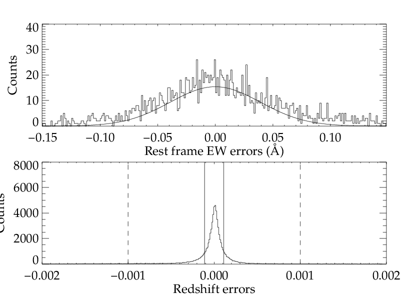
We also used our Monte Carlo simulation to study the errors in our measured line parameters. Figure 9 shows histograms of the differences in the injected and measured rest frame equivalent widths (top panel) and redshifts (bottom panel). The rest frame equivalent width plot contains the errors for over 1750 Mg ii and singlets fit by hand. The overplotted zero mean Gaussian has a width equal to the standard deviation of the sample, . The plot shows no significant biases. The redshift plot contains errors for the first 200 simulated spectra for each QSO in our Monte Carlo completeness simulation (corresponding to over 67,500 systems). The solid vertical lines are separated by one pixel (), and the dotted vertical lines represent the precision given in Table 2. The standard deviation of the sample is .
IV. Results
IV.1. Population Statistics


Figure 10 shows raw histograms of the rest frame equivalent width (top panel) and redshift (bottom panel) distribution of the sample’s 110 Mg ii systems, before corrections for incompleteness (proximate system not included). The rest frame equivalent widths range from (SDSS0140-0839, ) to (CFQS1509, ). The sample contains Mg ii systems with redshifts over 5, with a maximum value of (SDSS1411, ). Three of these systems come from SDSS1411’s sightline, which contains four high redshift systems at 5.06, 5.25, and 5.33.
Figure 11 displays the relationship between the rest frame equivalent widths of the Mg ii singlets and velocity spreads (measured to where the absorption troughs intersect the continuum) of this sample. These velocity spreads have been adjusted for FIRE’s resolution of 50 km/s. The overplotted line is the sigma-clipped best fit line, given by
| (8) |
This slope and the strong correlation present in Figure 11 are consistent with previous results from Ellison [15] at lower redshifts, . We incorporated this measured correlation and scatter into our Monte Carlo completeness simulations described in III.2.1 to ensure that our injected systems resembled true systems from the sample. (Strong injected systems were modeled as a blend of narrow components with total velocity spread drawn from the distribution specified by Equation 8).
IV.2. Incorporating Variable Completeness in Population Distributions
When calculating the line density and equivalent width distributions, we first define the true number of systems in the universe within a binned region centered on as . If the total redshift path in bin is , and the total range of rest frame equivalent width in the bin is , then the population densities are given by
| (9) | |||||
| (10) | |||||
| (11) |
Using our completeness matrices we may relate these quantities to the expected number of survey detections. A complete derivation of this method is given in the Appendix. In summary, for an incomplete survey with path length given by , the number of detected systems in a bin is estimated as
| (12) |
The average completeness is defined as the ratio between this and the true number of systems ,
| (13) | |||||
| (14) |
Our Monte Carlo calculations give us access to (which in turn leads to ) with an important caveat. The average completeness within a bin is a weighted integral of the fine grained completeness across the bin, with weighting function . If the true completeness varies within a bin, then that average depends on the very function we are trying to calculate.
There are three ways around this dilemma: (1) We can assume that the completeness is constant across all sightlines and across the full breadth of the bin. Since the quality of the data varies largely from spectrum to spectrum, this assumption is not warranted. (2) We can assume that the population density within the bin is approximately constant. With this approximation, the population density in bin reduces to
| (15) |
This is the method employed in the recent C iv study of Simcoe et al. [61] when considering variable completeness within bins, and implicitly in any previous Mg ii studies which employed the hard threshold completeness floor given previously in Equation 6. (3) We can compensate for this variability in both completeness and absorber line density by employing a maximum likelihood estimate to a functional form of the frequency distribution in the calculation of the average completeness in Equation 14.
We explored methods (2) and (3) using the maximum-likelihood estimates of the frequency distribution defined later in this paper. Figure 12 shows the effect of these corrections on for the range . “X”-shaped points indicate our values prior to completeness correction; the triangles show completeness-corrected values with no user-screening (i.e., using rather than for the correction and not adjusting for false positives, as described next section). The squares and diamonds include the full completeness and false positive corrections using methods (2) and (3) respectively to treat intra-bin variation in the frequency distribution. Apparently this effect contributes a negligible correction to our calculations of the population densities when compared with the sample’s Poisson errors. For this reason, we will instead use method (2) for calculating unless otherwise stated.
IV.3. Adjusting for False Positives
In the previous section, we calculated population densities in the presence of variable completeness, but did not account for false positives. Adjustments for false positives once again require Equations 9 to 11 for the population densities, but with the true number of systems calculated as
| (16) |
where is the number of detected Mg ii systems in bin , is the number of rejected candidates, is the average completeness, is the automated line identification finding probability, and is the user acceptance rate of non-Mg ii candidates. All average values here are path length weighted (once again employing the assumption that the population distributions are approximately constant across the bin). A full derivation of this formula is given in the Appendix. Note that as (the user correctly rejects all false positives), this reduces to the previous formula, .

Figure 12 shows the effect of user errors on the resultant for the rest frame equivalent width range . As previously stated, the triangles employ neither Equation 16 above to adjust for accepted false positives, nor the full completeness , which accounts for user rejection of real Mg ii systems. The squares include both of these user error corrections. The rejection of real Mg ii systems is by far the more dominant of these two effects, with the correction for accepting false positives negligible compared to the Poisson error bars (indicative of conservative users hesitant to accept anything suspect). The correction is the largest in the lowest redshift bin, where the effective sensitivity is (as shown later), the poorest regime in this survey. As the sensitivity improves with redshift, the user adjustments decrease in magnitude. Across the full range of redshifts and equivalent widths, the user accepts of all real Mg ii systems. The presented error bars include completeness errors, but at , these are subdominant to the Poisson errors.
IV.4. d2N/dzdW

Figure 13 displays the rest frame equivalent width distribution for the entire survey with all appropriate corrections applied. Table 3 contains these calculated values. The distribution is fit well by a simple exponential at , but shows a relative overabundance of systems in the highest equivalent width bin.
Full Sample and Redshift Cuts
0.42 0.05-0.64 50.0 47 1.5700.272
0.94 0.64-1.23 81.2 28 0.5940.119
1.52 1.23-1.82 82.6 14 0.2910.080
2.11 1.82-2.41 82.6 9 0.1870.064
2.70 2.41-3.00 82.6 4 0.0830.042
4.34 3.00-5.68 82.6 6 0.0270.011
0.43 0.05-0.64 44.3 22 1.7120.412
0.94 0.64-1.23 77.5 8 0.3810.137
1.53 1.23-1.82 79.2 7 0.3230.125
2.12 1.82-2.41 79.2 4 0.1870.094
2.71 2.41-3.00 79.2 2 0.0930.066
4.34 3.00-5.68 79.2 5 0.0510.023
0.41 0.05-0.64 61.7 17 1.6340.414
0.94 0.64-1.23 91.1 11 0.7230.222
1.52 1.23-1.82 92.0 6 0.3910.161
2.11 1.82-2.41 92.0 2 0.1300.092
2.70 2.41-3.00 92.0 1 0.0650.065
4.34 3.00-5.68 92.0 1 0.0140.014
0.41 0.05-0.64 61.0 7 1.4290.559
0.94 0.64-1.23 90.7 5 0.6940.313
1.52 1.23-1.82 91.5 1 0.1380.138
2.11 1.82-2.41 91.5 2 0.2750.195
2.70 2.41-3.00 91.5 1 0.1380.138
4.34 3.00-5.68 91.5 0 0.030
Exponential Parameterization of the Distribution
0.68aaParameter fits from Nestor et al. [44] 0.366-0.871 0.5850.024 1.2160.124
1.10aaParameter fits from Nestor et al. [44] 0.871-1.311 0.7410.032 1.1710.083
1.60aaParameter fits from Nestor et al. [44] 1.311-2.269 0.8040.034 1.2670.092
2.51 1.947-2.975 0.9350.150 1.7550.081
3.46 3.150-3.805 0.7660.152 1.9520.105
4.78 4.345-5.350 0.7000.180 1.8110.141
3.24 1.947-6.207 0.8240.090 1.8270.059
Using maximum-likelihood techniques, we fit the equivalent width distribution using the functional form
| (17) |
We first calculated a maximum likelihood estimate of , and then calculated by insisting that the pathlength-weighted integral of this population distribution equal the number of found systems,
| (18) |
This process yielded values of and . Figure 13 displays this maximum likelihood fit plotted over the binned, completeness-corrected values.
We can use this result to calculate an effective equivalent width sensitivity for the full survey. Suppose one assumes that the survey’s limiting equivalent width is characterized by a single number that is constant at all redshifts and along all sightlines, . Then according to Equation 4,
| (19) |
In this regime, the maximum likelihood estimate of may be solved analytically as
| (20) | |||||
| (21) |
where is the average rest frame equivalent width of our sample [42]. We define the effective sensitivity of our survey as the value of in this equation that, given our calculated value of , would lead to the average rest frame equivalent width that we observe. For our reported values of and , we obtain an effective sensitivity of across the full survey.


In Figure 14, we subdivide into three different redshift ranges; , , and . Table 3 lists the values plotted. We also refit MLE estimates of for each of these regions (, , and , respectively), and recalculated the effective rest frame equivalent width sensitivities in each region (, , and , respectively). In Figure 15 we plot , and include previously published values from Nestor et al. [44], to connect our results with lower redshifts. Table 4 contains a summary of all these values.
Clearly the trend of increasing seen at lower redshift does not extrapolate to earlier epochs. Rather, it exhibits a peak value of at and smaller values at both higher and lower redshifts. A larger value of corresponds to a flatter equivalent width distribution with a larger fractional contribution from high- absorbers. It appears that going back in time, evolves to include more strong Mg ii systems until a maximum is reached at , after which the relative frequency of strong systems once again declines. It is tempting to associate this rise and fall of the strong Mg ii systems with the concurrent rise and fall of the global star formation rate; we will explore this association in detail below.
To quantify ’s redshift evolution, we followed the lead of Nestor et al. [44] and performed a MLE fit to
| (22) |
The best fit parameters for this from were , , and . The parameters and were anti-correlated, with . In Figure 15 we overplotted this best fit with a solid line, as well as the analogous MLE fit of Nestor et al. [44] to his data with a dashed line. The results show that a simple power law in does not adequately capture ’s redshift evolution over the full redshift range now available. Rather, there is evidence that the overall distribution is steepening towards higher .
To examine evolution in the overall normalization of the frequency distribution, we also fit our data to the functional form
| (23) |
This exercise yielded , , and . As is usual, these multi-dimensional MLE fits yield large errors for small samples such as ours, but within these limitations we do not see statistically significant evidence for redshift evolution in the normalization of number counts.
IV.5. dN/dz and dN/dX

Figure 16 displays the completeness-corrected, binned values of for our Mg ii sample in three different rest frame equivalent width ranges. These ranges were chosen for easy comparison with published SDSS Mg ii surveys at lower redshift [44, 50], which are overplotted. Table 5 contains the values of the data points in this figure.
We also fit the absorber line density to a simple polynomial,
| (24) |
We calculated a maximum likelihood fit of , and then calculated by insisting that our redshift path density integrated against this absorber cross section equal the total number of systems located,
| (25) |
where is the total rest equivalent width range probed. We performed this MLE fit over our full survey, and over the three rest frame equivalent width ranges from Figure 16. Table 6 contains these MLE fits, as well as the analogous fits from Prochter et al. [50]. These fits are also overplotted with dashed lines in Figure 16.

| Number | |||||
|---|---|---|---|---|---|
| Å | |||||
| 2.231 | 1.947-2.461 | 47.3 | 4 | 0.3620.193 | 0.1150.061 |
| 2.727 | 2.461-2.975 | 69.1 | 8 | 0.4860.176 | 0.1410.051 |
| 3.457 | 3.150-3.805 | 77.9 | 10 | 0.4530.146 | 0.1190.038 |
| 4.786 | 4.345-5.350 | 76.9 | 4 | 0.3870.195 | 0.0880.045 |
| 2.232 | 1.947-2.461 | 65.5 | 5 | 0.3430.156 | 0.1090.049 |
| 2.723 | 2.461-2.975 | 84.6 | 3 | 0.1490.087 | 0.0430.025 |
| 3.458 | 3.150-3.805 | 89.9 | 11 | 0.4320.132 | 0.1130.035 |
| 4.779 | 4.345-5.350 | 89.6 | 5 | 0.4150.187 | 0.0950.043 |
| 2.231 | 1.947-2.461 | 70.4 | 8 | 0.5090.185 | 0.1610.059 |
| 2.722 | 2.461-2.975 | 87.5 | 12 | 0.5780.170 | 0.1680.050 |
| 3.459 | 3.150-3.805 | 92.0 | 12 | 0.4610.135 | 0.1210.035 |
| 4.776 | 4.345-5.350 | 91.5 | 4 | 0.3250.164 | 0.0740.037 |
Line Density Evolution
| (Å) | (Å) | |||
|---|---|---|---|---|
| 1.17aaParameter fits from Prochter et al. [50], with corresponding upper and lower confidence intervals. This survey’s results include errors. | 1.00-1.40 | 0.35-2.3 | ||
| 1.58aaParameter fits from Prochter et al. [50], with corresponding upper and lower confidence intervals. This survey’s results include errors. | 1.40-1.80 | 0.35-2.3 | ||
| 1.63aaParameter fits from Prochter et al. [50], with corresponding upper and lower confidence intervals. This survey’s results include errors. | 1.00+ | 0.35-2.3 | ||
| 2.08aaParameter fits from Prochter et al. [50], with corresponding upper and lower confidence intervals. This survey’s results include errors. | 1.40+ | 0.35-2.3 | ||
| 2.52aaParameter fits from Prochter et al. [50], with corresponding upper and lower confidence intervals. This survey’s results include errors. | 1.80+ | 0.35-2.3 | ||
| Full Range | 1.9-6.3 | |||
| 0.45 | 0.30-0.60 | 1.9-6.3 | -0.1040.937 | 0.4820.644 |
| 0.79 | 0.60-1.00 | 1.9-6.3 | 0.9280.889 | 0.0930.121 |
| 1.82 | 1.00+ | 1.9-6.3 | -0.7460.857 | 1.3011.555 |
In addition, we calculated the comoving absorber line density . These completeness-corrected, binned results are shown in Figure 17, with the corresponding results from Nestor et al. [44] and Prochter et al. [50] once again overplotted. The dashed horizontal lines show the straight mean of our data combined with those of Nestor et al. [44]. As in the usual interpretation, a constant value of corresponds to a population with no comoving evolution.
The smaller rest frame equivalent width systems () show remarkably little evidence of cosmic evolution over the entire range of redshifts probed by these surveys. For the low end Å sample the data are consistent () with a constant value of , and only standard deviation. The same is true for , where uncertainty from incompleteness is even smaller. In this range, with and scatter around a constant value. In contrast, the large rest frame equivalent width systems () show significant evolution over ours and previous surveys; for a constant value of over our survey and Nestor’s, and increases to if Prochter’s Å data are further included. Table 5 contains the values of our new data points from this figure.
V. Discussion
The initial results of our 46 sightline survey demonstrate that Mg ii absorbers were already commonplace at . Rather remarkably, the comoving number density of Mg ii absorbers with Å is completely flat at with scatter of only between and , a period of Gyr. In contrast, the stronger Mg ii absorbers grow in number density by a factor of from the present towards , after which they drop off by a comparable amount toward . The differential nature of the evolution between strong and weak systems is reflected in the equivalent width distribution, which is more shallow (higher ) at than it is at lower and higher redshifts. The change in total number counts is still small since the strong systems are subdominant at all redshifts.
Local surveys of absorber-galaxy pairs typically find Mg ii systems in the extended kpc haloes of galaxies with or slightly below [3, 62, 10, 63, 30]. According to the CDM picture of structure formation, galaxies resembling present-day systems should be rare at . Assuming that Mg ii absorbers are still found near galaxies at these epochs, it follows that the typical galaxy giving rise to Mg ii absorption in the early universe must look quite different from the systems studied locally.
The constancy of for weak absorbers implies that the product of the comoving number density and physical cross section of absorbing regions also remains constant. A simple interpretation is that these absorbers arise near the assembling progenitors of present-day galaxies. This would require that galaxy haloes were populated with Mg ii very early in their history, and that the absorption properties were established before their stellar and ISM components were fully formed.
A detailed analysis of absorption in individual Mg ii systems will be presented in a companion paper; however in a qualitative sense it appears that Mg ii systems at are very similar to those at low redshift, in contrast to the galaxy population. This either requires the absorption systems to persist in a steady state over much of the Hubble time, or else be replenished periodically. If Mg ii systems are replenished through stellar feedback, this process must proceed in a way that does not produce a cumulative growth of the gas radius and/or filling factor of Mg ii . This would seem to be a challenge unless some portion of the gas re-accretes and cycles back into the galaxy [46] or else the Mg ii -bearing clouds are out of equilibrium and transition to lower densities and higher ionization states.
V.1. Mg ii and Cold Accretion Flows
Recently Mg ii has been suggested as a candidate tracer of “cold” accretion onto galaxies, since its relatively low ionization potential (1.1 Ryd) does not allow for large Mg ii fractions at high . Cold accretion is thought to be the dominant mode of gas transport onto galactic disks; it is particularly efficient in the early universe for small, growing haloes [32, 14, 17] and could provide another “renewable” source for cool absorbers. While attractive, this model for the Mg ii population faces some complications at the high redshifts probed by our survey. Principally, at these epochs, even though cold accretion is much stronger [14, ;] and may present a larger absorption cross section, the heavy element content of the IGM gas reservoir is quite low: at [58] and even lower at earlier times. In general, cold streams may manifest as metal-poor Lyman limit systems [19] more prominently than Mg ii systems. We may already be seeing this phenomenon, in that the density of Lyman limit systems and Mg ii are of comparable magnitude at low redshift, but unlike Mg ii , the LLS density continues increasing with redshift [49, 53] beyond .
Tinker & Chen [65] present a model of the evolving Mg ii population which maps Mg ii absorbers onto the dark matter halo mass function, as a way of studying evolution of the underlying galaxies. In their model, most Mg ii absorbers arise in haloes with which are presumed to be growing via cold accretion. Shock heating reduces the supply of Mg ii in larger mass haloes, an effect which is required to match the observed anti-correlation between galaxy mass and in the local universe [5, 22]. However, an additional suppression of absorption efficiency is also needed in low mass () haloes to offset the rapidly rising halo mass function in this regime.

This low-mass cutoff halts the overproduction of weak Mg ii systems in low mass haloes, aligning the model with observations at . However at high redshift, a larger portion of the mass is concentrated in these very haloes, most of which fall below the low-mass cut for harboring Mg ii absorption. As a direct consequence, the simple halo-occupation model under-predicts the measured at by orders of magnitude, as seen in Figure 18. It may be possible to reconcile the model by boosting the absorption efficiency of small mass haloes at early times, or else growing the absorption cross-section per halo from of the virial radius at to at early times. However these solutions are not physically motivated a priori and would need further exploration.
It appears Mg ii will be a difficult ion to use as a tracer of cold accretion flows. The competition between declining IGM metal abundance and rising cold accretion cross section at earlier times would require a fine balance to achieve the very flat trend we observe in . While this solution is possible in principle, it will be difficult to interpret.
V.2. Comparison with Known Galaxy Populations
When comparing our Mg ii number counts with galaxy populations, another approach is to skip the halo mass function altogether, and apply simple empirical scalings between Mg ii gas halo size, covering fraction, and galaxy luminosity to predict . The model cross sections are integrated over measured luminosity functions as a function of redshift.
To estimate each galaxy’s cross section, we use the scalings of Chen et al. [10], who studied a spectroscopic sample of 94 galaxy-absorber pairs at . Chen found that galaxies with higher band luminosities possess more extended Mg ii absorbing haloes [62, see also], and fit the extent of these gaseous haloes to a Holmberg-like scaling,
| (26) |
where kpc, , and is the luminosity associated with objects of at their survey redshift. We use Equation 26 together with measurements of the band luminosity function at increasing redshift [48, 72, 20, 71, 39] to calculate the abundance and cross section of absorbers and compare with our measurements of .
When extrapolating Equation 26 to higher redshift, we explored two ways of evolving the scaling. In the simplest approach, and are fixed at all redshifts, so galaxies with always have haloes of radius . According to the studies cited above, evolves with redshift toward brighter values in the past. With a constant value of defining the halo scale, this implies that galaxies at will have gas haloes increasingly larger than (i.e. kpc) in the more distant past. For this reason, we will find it useful to define the term , which denotes the gas radius of an galaxy at any redshift.
In the second approach, we associate gas haloes of size with galaxies of from the luminosity function at each epoch. This is equivalent to setting and replacing with in the notation above. Since increases with , in this scenario galaxies at a fixed luminosity would have smaller gas haloes in the past than in the present day.
We next model the absorbers’ covering fraction as a function of galaxy impact parameter , using an empirical approximation based on the results of Chen et al. [10]:
| (27) |
Briefly, each galaxy has a central core of radius within which ; between (the core radius) and (the halo boundary) the covering fraction declines linearly to zero. We assume mimics ’s scaling with in both scenarios considered, but with kpc.
The total absorption cross section presented by a galaxy is then
| (28) | |||||
| (29) |
Here is the cross section of an galaxy’s gas halo, which may evolve with redshift but does not depend on luminosity,
| (30) | |||||
| (31) |
The quantity is the average covering fraction of the gaseous halo, and is with the given values of and .

The Mg ii frequency may be derived by combining this per-galaxy cross section with the band luminosity function :
| (32) |
where is a lower luminosity cutoff, which is not specified a priori, but rather chosen to match the normalization of the observed . Using a Schechter [56] function for , we may calculate the linear density as
| (33) |
where is the upper incomplete gamma function. This expression is similar to one derived in Churchill et al. [12], the only difference being the factor of correction for partial covering.
We evaluated Equation 33 using the band luminosity functions of Poli et al. [48], Wolf et al. [72], Gabasch et al. [20], Willmer et al. [71]; and Marchesini et al. [39] to calculate from to . The results are shown in Figure 19, with triangles and circles representing the predicted and measured (for Å), respectively. The solid curves indicate the predicted evolution based on redshift-dependent fits to the luminosity function parameters from Giallongo et al. [25] and Gabasch et al. [20].
The top panel shows results for the model where the luminosity associated with -sized haloes tracks . In this case, the observed and predicted match best when . However the model predicts a downward evolution in with that is slightly steeper than what is observed. This means that the typical cross section per galaxy is higher than the model predicts at high redshift, suggesting that either the haloes are growing slightly in radius or their filling factors are increasing.
The bottom panel shows the simple model where the fiducial luminosity associated with haloes is fixed at all redshifts. Our best fit is obtained with , almost an order of magnitude larger than the previous model. The redshift dependence for this model is flatter, in better agreement with our survey data. The relatively high value of indicates that a large population of very low luminosity galaxies need not be invoked to explain the frequency of Mg ii systems in this model; for the most part, all Mg ii systems surround galaxies we can readily observe, even at high redshift.
This picture could be invalidated if significant numbers of Mg ii systems are discovered near galaxies with . However to date such dwarf-Mg ii associations have not been established except in a few cases. Even in Chen et al. [10]’s sample of 94 pairs, of the galaxies meet this criterion. They are predominantly at very small impact parameter ( kpc) and even then show only coverage (in contrast to our model, in which the coverage is out to kpc).
The points in Figure 19 apply for Å since this was the range over which the correlation was first determined. However we have also seen that if we restrict further to Å, evolves to a peak at and declines thereafter. Neither of our halo models is able to reproduce this feature, which indicates that other physics must be at play. If the systems giving rise to the strong absorbers are contained in the band luminosity function, then their gas cross section and/or covering fraction must rise and then fall again. Alternatively they may reflect systems whose comoving number density rises and falls without being picked up in rest frame band surveys.
Rather than start with a halo and coverage model and derive , we may instead start with the observed Mg ii and estimate the effective size of gaseous haloes. To do this, we define the effective halo radius of an absorber according to
| (34) | |||||
| (35) |
where is the luminosity-weighted covering fraction and is luminosity-weighted gaseous halo radius.

In Figure 20, we plot the effective halo radius as a function of redshift, normalized by the radius calculated in the lowest redshift bin. We use an average of the redshift evolution luminosity function models of Giallongo et al. [25] and Gabasch et al. [20] in conjunction with four different lower luminosity cutoffs: 0.001, 0.01, 0.1, and 1.0 . All four choices of a lower luminosity cutoff result in the effective absorbing halo radius increasing by from today to , and then slightly decreasing again (although the error bars are too large to consider this final decrease statistically significant). This increase in effective halo radius must result from either an increase in the luminosity-weighted covering fraction at earlier times, or an increase in the extent of the gaseous absorbing haloes at earlier times. Although the lower luminosity cutoff still remains a free parameter in this model, the strong quantitative agreement of the normalized effective halo radii across three orders of magnitude in suggests this feature is largely independent of the lower luminosity cutoff employed.
V.3. Deriving the SFR Density from dN/dX

Thus far we have focused the discussion on moderate strength Mg ii absorbers which do not evolve with redshift. But the systems with Å do evolve, with a characteristic rise and fall that suggests a possible connection to the cosmic star formation rate density
This connection is also explored in Ménard et al. [40], where a method is outlined for deriving the SFR density from the Mg ii population distribution by establishing a connection between Mg ii rest frame equivalent width and [O ii] luminosity, which previous studies have shown may be used as a gauge of the SFR [21, 31, 27, 33, 41]. Since the detection of Mg ii using spectroscopic absorption does not depend on luminosity, distance, or dust extinction, such a probe would represent a valuable asset in pinning down the star formation history of the universe.
In their paper, the authors search for [O ii] emission lines from Mg ii host galaxies imprinted on a sample of QSO spectra containing over 8500 known Mg ii absorbers at redshifts . They detect a correlation between the absorber strength and the median [O ii] luminosity surface density , which they fit to the functional form
| (36) |
where ergs s-1 kpc2 and . The authors calculate the co-moving [O ii] luminosity density probed by Mg ii absorbers from this by using the completeness corrected population distribution from Nestor et al. [44] according to
| (37) |
Finally, they convert this luminosity density to a luminosity and derive a SFR density by using an average over scalings from Zhu et al. [73],
| (38) |
Using this technique, Ménard et al. [40] convert the data from Quider et al. [51] to SFR densities, and then overplot SFR density data provided in Hopkins [26]. The results show agreement up to .
More recently, López & Chen [37] have argued that the - correlation reported in Ménard et al. [40] does not reflect a causal connection between Mg ii absorption and star formation. Rather, they demonstrate that the observed correlation could plausibly arise from a combination of the empirically observed decline in at increasing galactocentric radius, and differential loss of galaxy light from the finite fiber aperture of the SDSS spectrograph. The authors run a large Monte Carlo simulation which reproduces the - relationship found in Ménard et al. [40].
Nevertheless, in light of the observed evolution in for Å, the large, likely non-gravitational velocity spreads observed for strong Mg ii systems (Figure 11), and the demonstrated connection between the strongest Mg ii absorbers and star forming galaxies [6, 45, 43], it is tempting to explore Menard’s method, while keeping in mind its possible limitations. The broad redshift range of our sample, combined with those of the SDSS studies, puts us in unique position to compare with the cosmic star formation history.
In Figure 21, we show the SFR density calculated using Equations 36 to 38, for Mg ii absorbers having Å (large circles). We also include previous results at low redshift from Nestor et al. [44] and Prochter et al. [50] over the same equivalent width range (smaller circles). For comparison, we overplot (with triangles) star formation rate densities obtained using recent determinations based on dropout counts from deep HST/WFC3 galaxy surveys at [7, 8], from a combination of ground-based spectroscopic and Spitzer MIPS 24 data at [52], and from the GALEX VIMOS-VLT Deep Survey at lower redshifts [1]. Menard’s transformation produces star formation rate densities in excellent agreement with the galaxy survey literature throughout the entire Mg ii absorption redshift search range probed, . These results do not conclusively demonstrate the accuracy of Equation 36—indeed application of Menard’s redshift dependent version of Equation 36 led to very high SFR values per absorber at and therefore predicted significantly higher SFR densities. However this exercise certainly suggests that the connection between Mg ii absorption and SFR is real for the strongest subset of Mg ii absorbers, and stretches over the full cosmic history.
Application of the Mg ii -SFR conversion to weaker absorbers () does not produce good agreement with galaxy surveys. These systems, as seen in Figure 17, exhibit remarkably little evolution in over all redshifts considered (). This suggests that any physical connection between Mg ii and star formation is mostly limited to the stronger end of the Mg ii equivalent width distribution. Indeed different astrophysical processes may govern the evolution of systems at high and low equivalent width, with the division occurring roughly at Å as suggested by Lovegrove & Simcoe [38] and Kacprzak & Churchill [29].
VI. Conclusions
Using FIRE, we have conducted an infrared survey of intervening Mg ii absorption toward the sightlines of 46 distant quasars with redshifts . The overall survey has an effective sensitivity of and a FWHM resolution of km/s. A combination of automated and human methods were used to identify and measure the properties of detected systems, and we performed extensive simulations to characterize our sample’s incompleteness and contamination from false positives. Our main findings are as follows:
- 1.
We find 110 isolated Mg ii systems (and one proximate system) ranging in rest equivalent width from to and in redshift from to , including 5 systems with .
- 2.
The population distribution resembles an exponential with a characteristic scale across the full survey. When we divide the survey into three redshift regions and combine our results with earlier results from Nestor et al. [44], we find that this characteristic scale rises with redshift until (where we find more strong systems), and then falls towards higher redshifts.
- 3.
For weaker Mg ii absorbers ( Å), the linear density is statistically consistent with no evolution, having with a scatter of only from to , a period of Gyr. In contrast, the stronger Mg ii absorbers ( Å) grow in number density by a factor of from the present towards , after which they drop off by a comparable amount toward . We interpret this as evidence of two distinct Mg ii populations, one which follows the global star formation rate density, and another which is nearly constant in comoving aggregate cross section.
- 4.
For strong Mg ii absorbers ( Å), the Mg ii-to-star formation rate scaling of Ménard et al. [40], together with our measured Mg ii frequency, agrees remarkably well with classically measured star formation density rates. While the recent analysis of López & Chen [37] cautions against a detailed exploration of this specific model, the excellent agreement with our measurements are highly suggestive of a connection between strong Mg ii absorption and star formation.
- 5.
For the weaker systems, models based on the predicted Mg ii occupation of dark matter haloes substantially under-predict at high redshifts. This discrepancy derives from the low absorption efficiency of small mass haloes locally (which are used for scaling), combined with the relative scarcity of high mass haloes in the early universe. To resolve the difference, the numerous low-mass haloes present at early times would need to have an enhanced absorption efficiency relative to present day levels.
- 6.
We are able to produce the observed more accurately using scaling relations between galaxy luminosity and halo size derived at low redshift, but integrated over appropriate high redshift determinations of the galaxy luminosity function. The correspondence is most accurate when the Mg ii absorbing halo’s size scales with a fixed, redshift-independent fiducial luminosity. Since increases with redshift, this implies that the effective gaseous halo of an galaxy is larger at earlier times. This model leaves the lower integration limit down the faint-end slope as a free parameter, set to match the normalization of . Our best match is for , so that large populations of low-luminosity galaxies are not strictly required to explain the observed Mg ii frequency, even at high redshift.
Our results indicate that Mg ii absorption remains commonplace in the early universe, having evolved relatively little over a period exceeding Gyr. This is in contrast to the C iv number counts, which decline by almost an order of magnitude over the same interval (K. Cooksey, private communication), and the density of the intergalactic H i Lyman alpha forest, which thickens markedly toward the epoch of reionization [2].
At low redshift, Mg ii absorbers are typically associated with kpc gas haloes surrounding galaxies. The Mg ii counts at high redshift can also plausibly be reproduced using fairly luminous galaxy populations. As will be shown in forthcoming work, the H i and other metal line properties of the high-redshift Mg ii systems also do not differ dramatically from the local population.
Yet the properties of the host galaxies themselves must have evolved substantially over the same period. As estimated by Gabasch et al. [20] brightens by a factor of , while declines by an order of magnitude over the redshift path where Mg ii has now been characterized. If the high redshift Mg ii absorbers are similarly associated with distinct galaxies, then the mass substructure within their dark matter haloes must have evolved significantly from to the present. Moreover, high resolution, rest-frame optical morphology studies of distant galaxies generally find that at fixed stellar mass, galaxies have smaller half light radii ( kpc at ) going backwards in time [36, 47, 18, 68].
It appears that as the stellar populations of typical galaxies grow from the inside out, the gaseous haloes of the same galaxies may be populated with metals very early on, and that the gas halo properties evolve much more weakly than do the galaxies themselves. If our hypothesis is correct that the observed may be recovered entirely by galaxies with , then it should be possible to observe such systems directly at intermediate redshifts, up to . Along with further spectroscopy to improve upon the modest sample sizes presented here, such follow up of Mg ii -selected galaxies may constitute a fruitful means for studying the concurrent buildup of the stellar and near field circum-galactic environments.
Appendix
Mathematical Framework for Variable Completeness
If our data set were 100% complete over the Mg ii redshift search range and rest frame equivalent width range spanned by a bin , then the expected number of Mg ii systems found within this bin would be given by the integral of the population distribution weighted by the sum of the regions probed along each sightline; more specifically,
| (A1) |
where the range of the integral, denoted by subscript , is over the redshift and rest frame equivalent width range of the bin. The total path in this bin would then be
| (A2) |
where the integral is now only over redshift. If we denote the change in equivalent width of the bin as , then the population density is estimated as
| (A3) |
With less than 100% completeness, the expected number of Mg ii systems found within this bin is instead
| (A4) | |||||
| (A5) |
We define the proportionality constant between and to be the average completeness in this bin,
| (A6) |
which leads to
| (A7) |
Mathematically, this is equivalent to calculating the average completeness across the bin using a probability density proportional to the product of the population distribution and the summed regions probed.
According to Equations A3 and A6 above, the completeness-corrected estimate of the population density is then
| (A8) |
Similarly, the estimates of the rest frame equivalent width distribution and the absorber line density are given by
| (A9) |
and
| (A10) |
If, as we argue in the main text, we assume that the population distribution is constant over bin when calculating , then the average completeness across the bin reduces to
| (A11) | |||||
| (A12) |
where we have employed the definition of from Equation 5 and the definition of the total path length given in Equation A2. Plugging this equation for back into Equation A8 for the population density above yields
| (A13) |
Mathematical Framework for False Positive Correction
Let denote the population density of false positives that our automated line identification system flags as potential candidates. The total number of false positives in bin is given by
| (A14) |
If is the probability of the user accepting a false positive in sightline at redshift and rest frame equivalent width , then the number of actual false positives that the user correctly identifies is
| (A15) |
Along with these, the user incorrectly identifies some real Mg ii systems as false positives,
| (A16) |
where is the automated completeness and is the total completeness as given in Equation 3, which also accounts for the user’s decisions.
In terms of accepted candidates, the number of correctly accepted Mg ii candidates follows from Equation A4,
| (A17) |
Along with these systems, the user incorrectly accepts some false positives, the number of which is given by
| (A18) |
As before, we will assume that the Mg ii and false positive population densities vary negligibly over the course of a single bin. Therefore, we may define the expected value of an arbitrary function over bin according to
| (A19) |
With this definition, the number of identified (real and spurious) Mg ii systems and false positives in bin are given by
Here, we have two equations and two unknowns, namely the number of real systems and true false positives . Solving for gives
| (A20) |
The population densities are then given by Equations 9 to 11 with this value substituted for .
References
- [1] Arnouts, S., et al. 2005, ApJ, 619, L43
- [2] Becker, G. D., Rauch, M., & Sargent, W. L. W. 2007, ApJ, 662, 72
- [3] Bergeron, J., & Boissé, P. 1991, A&A, 243, 344
- [4] Bochanski, J. J., et al. 2009, PASP, 121, 1409
- [5] Bouché, N., Murphy, M. T., Péroux, C., Csabai, I., & Wild, V. 2006, MNRAS, 371, 495
- [6] Bouché, N., Murphy, M. T., Péroux, C., Davies, R., Eisenhauer, F., Förster Schreiber, N. M., & Tacconi, L. 2007, ApJ, 669, L5
- [7] Bouwens, R. J., et al. 2010, ApJ, 725, 1587
- [8] —. 2011, ApJ, 737, 90
- [9] Bowen, D. V., & Chelouche, D. 2011, ApJ, 727, 47
- [10] Chen, H.-W., Helsby, J. E., Gauthier, J.-R., Shectman, S. A., Thompson, I. B., & Tinker, J. L. 2010a, ApJ, 714, 1521
- [11] Chen, H.-W., Wild, V., Tinker, J. L., Gauthier, J.-R., Helsby, J. E., Shectman, S. A., & Thompson, I. B. 2010b, ApJ, 724, L176
- [12] Churchill, C. W., Rigby, J. R., Charlton, J. C., & Vogt, S. S. 1999, ApJS, 120, 51
- [13] Cushing, M. C., Vacca, W. D., & Rayner, J. T. 2004, PASP, 116, 362
- [14] Dekel, A., et al. 2009, Nature, 457, 451
- [15] Ellison, S. L. 2006, MNRAS, 368, 335
- [16] Elston, R., Bechtold, J., Hill, G. J., & Ge, J. 1996, ApJ, 456, L13
- [17] Faucher-Giguere, C., & Keres, D. 2010, ArXiv e-prints
- [18] Franx, M., van Dokkum, P. G., Schreiber, N. M. F., Wuyts, S., Labbé, I., & Toft, S. 2008, ApJ, 688, 770
- [19] Fumagalli, M., O’Meara, J. M., & Prochaska, J. X. 2011, Science, 334, 1245
- [20] Gabasch, A., et al. 2004, A&A, 421, 41
- [21] Gallagher, J. S., Hunter, D. A., & Bushouse, H. 1989, AJ, 97, 700
- [22] Gauthier, J., Chen, H., & Tinker, J. L. 2009, ApJ, 702, 50
- [23] Gauthier, J.-R., & Chen, H.-W. 2011, MNRAS, 1604
- [24] Gauthier, J.-R., Chen, H.-W., & Tinker, J. L. 2010, ApJ, 716, 1263
- [25] Giallongo, E., Salimbeni, S., Menci, N., Zamorani, G., Fontana, A., Dickinson, M., Cristiani, S., & Pozzetti, L. 2005, ApJ, 622, 116
- [26] Hopkins, A. M. 2004, ApJ, 615, 209
- [27] Hopkins, A. M., et al. 2003, ApJ, 599, 971
- [28] Jiang, L., Fan, X., Vestergaard, M., Kurk, J. D., Walter, F., Kelly, B. C., & Strauss, M. A. 2007, AJ, 134, 1150
- [29] Kacprzak, G. G., & Churchill, C. W. 2011, ArXiv e-prints
- [30] Kacprzak, G. G., Churchill, C. W., Evans, J. L., Murphy, M. T., & Steidel, C. C. 2011, MNRAS, 416, 3118
- [31] Kennicutt, Jr., R. C. 1992, ApJ, 388, 310
- [32] Kereš, D., Katz, N., Weinberg, D. H., & Davé, R. 2005, MNRAS, 363, 2
- [33] Kewley, L. J., Geller, M. J., & Jansen, R. A. 2004, AJ, 127, 2002
- [34] Kondo, S., et al. 2008, in Astronomical Society of the Pacific Conference Series, Vol. 399, Panoramic Views of Galaxy Formation and Evolution, ed. T. Kodama, T. Yamada, & K. Aoki, 209
- [35] Lanzetta, K. M., Turnshek, D. A., & Wolfe, A. M. 1987, ApJ, 322, 739
- [36] Law, D. R., Steidel, C. C., Shapley, A. E., Nagy, S. R., Reddy, N. A., & Erb, D. K. 2011, ArXiv e-prints
- [37] López, G., & Chen, H.-W. 2011, ArXiv e-prints
- [38] Lovegrove, E., & Simcoe, R. A. 2011, ApJ, 740, 30
- [39] Marchesini, D., et al. 2007, ApJ, 656, 42
- [40] Ménard, B., Wild, V., Nestor, D., Quider, A., Zibetti, S., Rao, S., & Turnshek, D. 2011, MNRAS, 417, 801
- [41] Mouhcine, M., Lewis, I., Jones, B., Lamareille, F., Maddox, S. J., & Contini, T. 2005, MNRAS, 362, 1143
- [42] Murdoch, H. S., Hunstead, R. W., Pettini, M., & Blades, J. C. 1986, ApJ, 309, 19
- [43] Nestor, D. B., Johnson, B. D., Wild, V., Ménard, B., Turnshek, D. A., Rao, S., & Pettini, M. 2011, MNRAS, 412, 1559
- [44] Nestor, D. B., Turnshek, D. A., & Rao, S. M. 2005, ApJ, 628, 637
- [45] Noterdaeme, P., Srianand, R., & Mohan, V. 2010, MNRAS, 403, 906
- [46] Oppenheimer, B. D., Davé, R., Kereš, D., Fardal, M., Katz, N., Kollmeier, J. A., & Weinberg, D. H. 2010, MNRAS, 406, 2325
- [47] Papovich, C., Dickinson, M., Giavalisco, M., Conselice, C. J., & Ferguson, H. C. 2005, ApJ, 631, 101
- [48] Poli, F., et al. 2003, The Astrophysical Journal Letters, 593, L1
- [49] Prochaska, J. X., O’Meara, J. M., & Worseck, G. 2010, ApJ, 718, 392
- [50] Prochter, G. E., Prochaska, J. X., , & Burles, S. M. 2006, The Astrophysical Journal, 639, 766
- [51] Quider, A. M., Nestor, D. B., Turnshek, D. A., Rao, S. M., Monier, E. M., Weyant, A. N., & Busche, J. R. 2011, AJ, 141, 137
- [52] Reddy, N. A., Steidel, C. C., Pettini, M., Adelberger, K. L., Shapley, A. E., Erb, D. K., & Dickinson, M. 2008, ApJS, 175, 48
- [53] Ribaudo, J., Lehner, N., & Howk, J. C. 2011, ApJ, 736, 42
- [54] Rubin, K. H. R., Weiner, B. J., Koo, D. C., Martin, C. L., Prochaska, J. X., Coil, A. L., & Newman, J. A. 2010, ApJ, 719, 1503
- [55] Sargent, W. L. W., Steidel, C. C., & Boksenberg, A. 1988, ApJ, 334, 22
- [56] Schechter, P. 1976, ApJ, 203, 297
- [57] Schneider, D. P., et al. 2010, AJ, 139, 2360
- [58] Simcoe, R. A. 2011, ApJ, 738, 159
- [59] Simcoe, R. A., et al. 2008, in Society of Photo-Optical Instrumentation Engineers (SPIE) Conference Series, Vol. 7014, Society of Photo-Optical Instrumentation Engineers (SPIE) Conference Series
- [60] Simcoe, R. A., et al. 2010, in Society of Photo-Optical Instrumentation Engineers (SPIE) Conference Series, Vol. 7735, Society of Photo-Optical Instrumentation Engineers (SPIE) Conference Series
- [61] Simcoe, R. A., et al. 2011, ArXiv e-prints
- [62] Steidel, C. C., Dickinson, M., & Persson, S. E. 1994, ApJ, 437, L75
- [63] Steidel, C. C., Kollmeier, J. A., Shapley, A. E., Churchill, C. W., Dickinson, M., & Pettini, M. 2002, ApJ, 570, 526
- [64] Steidel, C. C., & Sargent, W. L. W. 1992, ApJS, 80, 1
- [65] Tinker, J. L., & Chen, H. 2010, ApJ, 709, 1
- [66] Tytler, D., Boksenberg, A., Sargent, W. L. W., Young, P., & Kunth, D. 1987, ApJS, 64, 667
- [67] Vacca, W. D., Cushing, M. C., & Rayner, J. T. 2003, PASP, 115, 389
- [68] van Dokkum, P. G., et al. 2010, ApJ, 709, 1018
- [69] Weiner, B. J., et al. 2009, ApJ, 692, 187
- [70] Weymann, R. J., Williams, R. E., Peterson, B. M., & Turnshek, D. A. 1979, ApJ, 234, 33
- [71] Willmer, C. N. A., et al. 2006, ApJ, 647, 853
- [72] Wolf, C., Meisenheimer, K., Rix, H.-W., Borch, A., Dye, S., & Kleinheinrich, M. 2003, A&A, 401, 73
- [73] Zhu, G., Moustakas, J., & Blanton, M. R. 2009, ApJ, 701, 86
- [74] Zibetti, S., Ménard, B., Nestor, D. B., Quider, A. M., Rao, S. M., & Turnshek, D. A. 2007, ApJ, 658, 161