Dynamics of Current Induced Magnetic Superstructures in Exchange-Spring Devices
Abstract
Thermoelectric manipulation of the magnetization of a magnetic layered stack in which a low-Curie temperature magnet is sandwiched between two strong magnets (exchange spring device) is considered. Controllable Joule heating produced by a current flowing in the plane of the magnetic stack (CIP configuration) induces a spatial magnetic and thermal structure along the current flow — a magneto-thermal-electric domain (soliton). We show that such a structure can experience oscillatory in time dynamics if the magnetic stack is incorporated into an electric circuit in series with an inductor. The excitation of these magneto-thermionic oscillations follow the scenario either of "soft" of "hard" instability: in the latter case oscillations arise if the initial perturbation is large enough. The frequency of the temporal oscillations is of the order of for current densities .
I Introduction
The electric control of magnetization on the nanometer length scale became a subject of intensive study after the seminal suggestion by Slonzewsky[1, 2] to use the spin torque transfer (STT) technique, where a current of spin-polarized electrons is injected into a magnetic material. Even though the magnetic tuning induced by the exchange interaction between the injected electrons and those that make the material magnetically ordered can only be achieved in a very small region, large current densities are needed to get a significant STT effect. Such current densities can be reached in electric point contacts where values of the order of A/cm3 have been achieved and the STT effect was detected.[3, 4] By a further increase of the current thermal Joule heating of the material becomes unavoidable. However, the fact that such heating can be precisely controlled by the bias voltage allows thermoelectrical manipulation of the magnetization direction based on the orientational phase transition in layered magnetic structures predicted in Ref. 5, 6, 7. It was shown there that in such structures with different Curie temperatures of the layers there can exist a finite temperature interval inside which the angle of the relative orientation of the layer magnetization depends on temperature, , changing reversibly with a change of temperature in the whole interval of angles from the parallel to the antiparallel orientation. As a result, by controlling the Joule heating by the bias voltage one may smoothly and reversibly control the relative magnetization angle in the whole angle interval . There was also suggested a thermal-electronic oscillator device based on this magneto-thermal effect in magnetic exchange spring structures.
In paper 8, for exchange-spring magnetic stacks[9] with an in-plane electric current flow (CIP) (see Fig. 1), it was predicted and investigated a possibility of generation of magnetic spatial superstructures (domains and solitons) the appearance of which and their parameters can be controlled by the bias voltage. In the present paper we study temporal dynamics of such spatial structures in the case that the exchange-spring magnetic stack is incorporated in an external circuit in series with an inductor [10]. Such oscillations can be understood as a realization of the bi-stability of an N-shaped IV curve of the device in the regime at which a large enough inductance of the circuit determines slow temporal variations of the current.
The structure of the paper is as follows. In Section II we present in short some peculiar features of the dependence of the magnetization orientation angle in the stack on temperature and some properties of the magnetic stack with a magnetic-thermal-electric domain (MTED) inside it needed for further considerations. In Section III we show that MTED loses its stability if the stack is incorporated in an external circuit with a large enough inductance. We develop there an adiabatic theory which allows an analytical description of the MTED dynamics.
II The magnetic-thermal-electric domain in the stack under Joule heating
The system under consideration has three ferromagnetic layers in which two strongly ferromagnetic layers 0 and 2 are exchange coupled through a weakly ferromagnetic spacer (layer 1) as is shown in Fig. 1. We assume that the Curie temperature of layer 1 is lower than the Curie temperatures of layers 0, 2; we also assume the magnetization direction of layer 0 to be fixed; this stack is under an external magnetic field directed opposite to the magnetization of layer 0. We require this magneto-static field to be weak enough so that at low temperatures the magnetization of layer 2 is kept parallel to the magnetization of layer 0 due to the exchange interaction between them via layer 1. At and this tri-layer is similar to the spin-flip "free layer" widely used in memory device application [11]. The stack is incorporated into an external circuit along which the total current flows through the cross-section of the layers:
| (1) |
where and are the magnetoresistance and the angle-independent resistance of the stack, is the angle between the magnetization directions of layers 0 and 2, is the voltage drop across the stack.
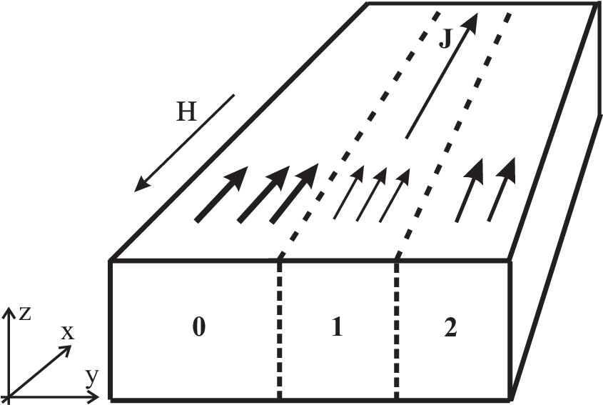
In paper [6], it was shown that parallel orientations of the magnetization in layers 0, 1 and 2 becomes unstable if the temperature exceeds some critical temperature . The magnetization direction in layer 2 smoothly tilts with an increase of the stack temperature in the temperature interval . The dependence of the equilibrium tilt angle between the magnetization directions of layers 0 and 2 on and the magnetic filed is determined by the equation [6]
| (2) | |||||
where
| (3) |
and
| (4) |
Here and are the widths and the magnetic moments of layers 1 and 2, respectively; is the exchange constant, is the exchange energy in layer 1, is the Bohr magneton, is Boltzmann’s constant, and is the lattice spacing. is a dimensionless parameter that determines the efficiency of the external magnetic in the misorientation effect under the consideration. It is a ratio between the energy of magnetic layer 2 in the external magnetic field and the energy of the indirect exchange between layers 0 and 2 (see Fig. 1).
The critical temperature of the orientation transition [12] is determined by the condition and is equal to
| (5) |
Taking experimental values (see Ref. 6) nm, nm, K, and magnetic field Oe one finds and the temperature interval K.
If the stack is Joule heated by current its temperature is determined by the heat-balance condition
| (6) |
where
| (7) |
and Eq. (2) which determines the temperature dependence of . Here is the voltage drop across the stack, is the heat flux flowing from the stack and is the total stack magnetoresistance. Here and below we neglect the explicit dependence of the magnetoresistance on considering the main mechanism of the stack resistance to be the elastic scattering of electrons by impurities. Below we drop the subscript "eff" at the magnetoresistance symbol . On the other hand, we consider the temperature changes caused by the Joule heating only in a narrow vicinity of which is sufficiently lower than both the critical temperatures and the Debye temperature.
Equations (6) and (2) define the IVC of the stack
| (8) |
where . The differential conductance is negative [6] if
| (9) |
where In this case the current-voltage characteristics of the stack (IVC) is N-shaped as is shown in Fig. 2.

In paper Ref. 8 it was shown that a homogeneous in space distribution of the magnetization direction, temperature and electric field along the spring-type magnetic stack becomes unstable and a magneto-thermal-electric domain (MTED) spontaneous arise [14] if the electric current flows in the plane of the layers (CIP-cofiguration) and the length of the stack exceeds the critical length
| (10) |
where is the thermal conductivity, is the magnetoresistivity and . Parameters of the MTED which arises in the stack, depend on the stack length and the voltage drop across it that allows to create and control magnetic structures in magnetic devices. Using Eq. (10) and the Lorentz ration ( and is the electron charge) one finds that
| (11) |
for a realistic experimental situation [26] , K, cm, .
The magnetic-thermal-electric domain (MTED) which determines the space distributions of the temperature and the magnetization direction angle which spontaneously arise in the magnetic stack, satisfies the following equation [8]:
| (12) |
in which current is found from the equation
| (13) |
supplemented with the periodic boundary condition ( is the coordinate along the stack, and are the length and the volume of the stack, respectively; the brackets indicate an average over along the whole stack of the length ).
The space distribution of the temperature and the magnetization direction angle in a long stack () with a MTED inside it is shown in Fig. 3.
In this limit () the MTED is of a trapezoid form with two planar segments of the length and () with two transition regions of the width (see Fig. 3).
Neglecting the contribution of the transition region in the total voltage drop across the stack, the dependence of the lengths and on the voltage drop across the stack can be written as
| (14) |
where , and , . In this approximation these formulas are valid in the range of where . The current and the voltage are coupled via current-voltage characteristics for the stack with MTED inside it. This dynamic IVC has a form close to a plateau in which the current coincides with the stabilization current [8] to an accuracy exponential in . The dynamic CVC can be presented in an implicit form as
| (15) |
Here , and the constants are of the order of while .

III Time Evolution of Magneto-Electric-Thermal Domain in Magnetic Stack
Here we assume that the magnetic stack is placed in series with an inductor. We also assume the bias-voltage regime that is the resistance of the external circuit in which the magnetic stack is incorporated can be neglected in comparison with that of the stack. In this case, taking into account that the temperature (here is the time) satisfies the equation of continuity of heat flow (see, e.g., Ref. 29), one obtains the following set of basic equations of the problem:
| (16) |
where
| (17) |
Here the dependence is given by Eq. (2). In the above equation is the current density which is independent of due to the condition of local electrical neutrality, is the cross-section area of the stack and is its length, is the heat capacity per unit volume, is the heat flux flowing from the stack, is its volume and is the stack magneto-resistivity (see Eq. (7)), is the inductance, and is the bias voltage; the definition of the brackets <…> is the same as in Eq.13.
The boundary condition to Eq. (16) is the continuity of the heat flux at the both ends of the stack (which is coupled to an external circuit with a fixed voltage drop over the stack). We shall not write down the expression for this condition, since the domain dynamics does not sufficiently depend on it. Instead, for the sake of simplicity we use the periodicity condition .
The set of equations Eq. (16) always has a steady-state solution which represent a magnetic-thermal-electric domain which satisfies Eq. (12). A study of the stability of this solution carried out using a linearized system Eq. (16) shows that the MTED loses its stability if the inductance exceeds some critical value where is the characteristic evolution time of the temperature[30]. Therefore, for the case this instability develops under conditions that the characteristic time of the current evolution is much longer than the temperature evolution time (their ratio is . Then any small fluctuation develops in such a way that after a time the domain recovers its initial trapezoidal form and only its length varies slowly with time . This fact makes it possible to obtain a reduced description of the nonlinear dynamics of a MTED as follows. We seek the solution of the first equation in Eq. (16) in the form
| (18) |
where is the solution of the equation which is obtained from Eq. (12) by the substitution ; the parameter governing the length of the domain is a slow function of the time which has to be found; is a correction which is small with respect to . Inserting Eq. (18) into the first equation in Eq. (16) and linearizing it one gets the following equation for :
| (19) |
where is a Hermitian operator with a periodic boundary condition:
| (20) |
(here and ). The requirement of the smallness of the ratio allows to find the needed equations describing the adiabatic MTED evolution.
The solution of Eq. (19) is found in the form of expansion
| (21) |
where are the eigenfunctions of which satisfy the Sturm-Liouville equation
| (22) |
Multiplying the both sides of Eq. (19) by from the left and averaging over the period one finds
| (23) |
where in terms of eigenfunctions is presented in Appendix A, Eq. (38).
As the eigenvalue is exponentially small (see Eq. (34)), from Eq. (19) it follows that the requirement is satisfied only when the right-hand side of the equation with is equal to zero:
| (24) |
Using Eq. (32) one sees that the right-hand side of the equation with is equal to zero and hence the factor in the left-hand side of it does not violate the above-mentioned requirement.
Taking into account the second equation in Eq. (16) and Eq. (24) together with Eqs.(37, 40) one finds a set of equations which describes the temporal dynamics of a MTED:
| (25) |
Here and (here is defined by Eq. (40)) may be written as
| (26) |
where the constant is
| (27) |
being of the order of the characteristic evolution time of the temperature , and is defined in Eq.(35).
Throughout the range of the existence of a trapezoidal MTED one has and the set of equations Eq. (25) can be reduced to an equation for the electric field which is coupled to the current via the voltage-current characteristic (see Eqs.(13,35)). Differentiating the first equation in Eq. (25) multiplied by with respect to , and inserting in the resulting expression the above-mentioned electric field as a new variable together with the second equation in Eq. (25) one obtains the following equation in the form of a linear oscillator with a nonlinear nonconservative term:
| (28) |
Here is the CVC of the magnetic stack with a MTED.
The static points of Eq. (28) and the second equation in Eq. (25) correspond to the domain solution and . As , in the range of inductance the factor in front of is negative and a domain is absolutely unstable. Here the critical inductance is
| (29) |
where is the electric field at which has a maximum that is at which . In this region the voltage drop across the magnetic stack oscillates and hence the length of the domain (see Eq. (14)) oscillates with an amplitude that increases in time. At the time when reaches either values (depending on the initial fluctuation) the domain disappears and the sample becomes homogeneous with temperatures or , respectively. Further temporal evolution of the system is described by the set of equations Eq. (16) an analysis of which for the case shows that the system exhibits stable large-amplitude spontaneous oscillations of the temperature , current current , magnetization direction , and the voltage drop across the stack , the oscillations being the same as those predicted in Ref. 6 for a magnetic stack in the absence of MTED.

Investigation of stability of the domain solution of Eq. (28) with the Poincare method (see, e.g., Ref. 32) shows that at there is an unstable limiting cycle in the phase plane the radius of which and hence it increases with a decrease of the inductance. From here and from the fact that at the domain is absolutely stable follows an existence of a second critical value of the inductance which limits the interval of the hard excitation of oscillations. Therefore, the range of values of the inductance is the region in which a stable MTED, an unstable limiting cycle, and a stable limiting cycle coexist. For this case, temporal developments of the MTED length , current and voltage drop across the magnetic stack are shown in Fig. 4 and Fig. 5.

IV Conclusion
We have considered the temporal evolution of magneto-thermo-electric domains which spontaneously arise in an exchange-spring magnetic stack with the electrical current flowing along the layers (CIP configuration). For the case that such a stack is incorporated in an electric circuit in series with an inductor we have found critical values of the inductance at which the magneto-thermal domain loses its stability. We have developed a perturbation theory in an adiabatic parameter (which is the ratio between the temperature and current characteristic evolution times) theory which allows to investigate the evolution of this instability into an oscillatory in time regime. The excitation of such magneto-thermionic oscillations follow the scenario of either “soft" of a “hard" instability; in the former case any perturbation results in a spontaneous transition to the oscillatory regime while in the latter case oscillations only appear if the initial perturbation is large enough. The frequency of the temporal oscillations of the magnetization direction in the stack is of the order of Hz.
V Acknowledgement.
Financial support from the EC (FP7-ICT-FET Proj. No. 225955 STELE), the Swedish VR, and the Korean WCU program funded by MEST/NFR (R31-2008-000-10057-0) is gratefully acknowledged.
Appendix A
According to Ref. 8 can be written as
| (30) |
where the function is a domain-wall type solution of Eq. (12) at and which has the following asymptotic
| (31) |
Here are the points of deflections of the curve so that is approximately the length of the "hot" section of a trapezoidal MTED having the maximal temperature and is the length of its "cold" section having the minimal temperature (see Fig. 3).
As one sees from Eq. (22) the function
in the former equation consists of two symmetrical "potential" wells of the width , separated by a barrier of the width of order of . In this case (see, e.g., Ref. 31) tunneling between the wells results in a splitting of each of the eigenvalues of a completely separated well into two neighboring ones, the splitting being proportional to , while the corresponding eigenfunctions are symmetric and antisymmetric combinations of the corresponding eigenfunctions of the separated left and right wells.
From the translation symmetry of the time independent equation Eq. (12) it follows that the eigenfunctions of the Hermitian operator include the function corresponding to the eigenvalue (it is easy to check inserting this function in the Eq. (22)). As it follows from Eq. (30) the eigenfunction is
| (32) |
where two functions in the right-hand side are eigenfunctions of the left and right wells when the tunneling is ignored. This is an antisymmetric eigenfunction () corresponding to the eigenvalue and hence the nearest eigenvalue is negative and the corresponding eigenfunction is symmetric:
| (33) |
while
| (34) | |||||
To express the eigenvalue in terms of the differential resistivity we use the following reasoning.
According to Eq. (13) the voltage-current characteristic of the stack with a MTED in it is
| (35) |
Differentiating the both sides of Eq. (35) and Eq. (12) with respect to one finds the differential resistivity of the magnetic stack with a MTED as
| (36) |
and an equation for
| (37) |
where the operator is given by Eq. (20).
Expanding in the form of the eigenfunctions (see Eq. (22)) one finds
| (38) |
Inserting it in Eq. (36) one finds
| (39) | |||||
Remembering that is exponentially small and hence it gives the main contribution to the sum with respect to one finds
| (40) |
References
- [1] J. C. Slonczewski, J. Magn. Magn. Mater. 159, L1 (1996), 195, L261 (1999).
- [2] L. Berger, Phys. Rev. B 54, 9353 (1996).
- [3] W. H. Rippard, M. R. Pufall, and T. J. Silva, Appl. Phys. Lett. 82, 1260 (2003).
- [4] I. K. Yanson, Y. G. Nadjuk, D. L. Bashlakov, V. V. Fisun, O. P. Balkashin, V. Korenivski, A. Konovalenko, and R. I. Shekhter, Phys. Rev. Lett. 95, 186602 (2005).
- [5] A. M. Kadigrobov, R. I. Shekhter, M. Jonson, and V. Korenivski, Phys. Rev. B 74, 195307 (2006).
- [6] A. M. Kadigrobov, S. Andersson, D. Radić, R. I. Shekhter, M. Jonson, and V. Korenivski, J. Appl. Phys. 107, 123706 (2010).
- [7] A. M. Kadigrobov, S. Andersson, H.-C. Park, D. Radić, R. I. Shekhter, M. Jonson, and V. Korenivski, arXiv:1101.5351.
- [8] A. M. Kadigrobov, R. I. Shekhter, and M Jonson, arXiv:1201.1514v1
- [9] J. E. Davies, O. Hellwig, E. E. Fullerton, J. S. Jiang, S. D. Bader, G. T. Zimanyi, and K. Liu, Appl. Phys. Lett. 86, 262503 (2005).
- [10] An experimental and analytical study of an analogous situation for thermo-electric domains (which arise due to a sharp temperature dependence of the resistance of pure metals at helium temperatures) was presented in the paper A. M. Kadigrobov, Yu. N. Chiang, and I. I. Logvinov, Sov. Phys. Solid State 28, 1903 (1986).
- [11] V. Korenivski and D. C. Worledge, Appl. Phys. Lett. 86, 252506 (2005).
- [12] The orientational phase transition in such a system induced by an external magnetic field was considered in Ref. 13.
- [13] G. Asti, M. Solzi, M. Ghidni, and F. M. Neri, Phys. Rev. B 69, 174401 (2004).
- [14] Electric domains in normal metals (see, e.g., the review Ref. 15) can also appear due to 1) structural [16] and magnetic [17, 18] transitions, 2) a sharp dependence of the resistance on at low temperatures and magnetic breakdown [19, 20, 21, 22, 23], 3) evaporation [24] and melting [25].
- [15] A. VI. Gurevich and R. G. Mints, Rev. Mod. Phys. 59, 941 (1987).
- [16] V. V. Barelko, V. M. Beibutyan, Yu. E. Volodin, and Ya. B. Zeldovich, Sov. Phys. Dokl. 26, 335 (1981).
- [17] R. Landauer, Phys. Rev. A 15 2117 (1977).
- [18] B. Ross and J. D. Lister, Phys. Rev. A 15, 1246 (1977).
- [19] A. A. Slutskin and A. M. Kadigrobov, JETP Lett. 28, 201 (1978).
- [20] A. M. Kadigrobov, A. A. Slutskin, and I. V. Krivoshei, Sov. Phys. JETP 60, 754 (1984).
- [21] Yu. N. Chiang and I. I. Logvinov, Sov. J. Low Temp. Phys. 8, 388 (1982).
- [22] V. V. Boiko, Yu. F. Podrezov, and N. P. Klimova, JETP Lett. 35, 649 (1982).
- [23] G. I. Abramov, A. V. Gurevich, V. M. Dzugutov, R. G. Mints, and L. M. Fisher, JETP Lett. 37, 535 (1983).
- [24] V. M. Atrazhev and I. T. Yakubov, High Temp. 18, 14 (1980).
- [25] G. I. Abramov, A. V. Gurevich, S. I. Zakharchenko, R. G. Mints, and L. M. Fisher, Sov. Phys. Solid State 27, 1350 (1985).
- [26] Typical densities of critical currents needed for the torque effect in point-contact devices are for the current perpendicular to the layers (CPP). The record low torque critical current in a nanopilar device was reported in Ref. 27 (see Ref. 28). In our paper we consider the case in which the torque effect is absent that is the torque critical current is higher than .
- [27] Z. Diao, Z. Li, S. Wang, Y. Ding, A. Panchula, E. Chen, L.-C. Wang, Y. Huai, J. Phys.: Condens. Matter 19, 165209 (2007).
- [28] D. C. Ralph and M. D. Stiles, J. Magn. Magn. Mater. 320, 1190 (2008).
- [29] L. D. Landau and E. M. Lifshitz, Electrodynamics of Continuous Media, Elsevier, Amsterdam (2009) §26.
- [30] For the realistic experimental parameters 1 J/Kcm3, 102 K, 10-5 cm and A/cm2 one has s.
- [31] L. D. Landau and E. M. Lifshitz, Quantum Mechanics, §50, Elsevier Science, Oxford (2003).
- [32] A. A. Andronov, A. A. Witt, and S. E. Khaikin, Theory of oscillations, Pergamon, Oxford (1966).