Bayesian Parameter Inference for Partially Observed Stopped Processes
Abstract
In this article we consider Bayesian parameter inference associated
to partially-observed stochastic processes that start from a set
and are stopped or killed at the first hitting time of a known set
. Such processes occur naturally within the context of a wide
variety of applications. The associated posterior distributions are
highly complex and posterior parameter inference requires the use
of advanced Markov chain Monte Carlo (MCMC) techniques. Our approach
uses a recently introduced simulation methodology, particle Markov
chain Monte Carlo (PMCMC) [1], where sequential Monte Carlo
(SMC) [18, 27] approximations are embedded within MCMC.
However, when the parameter of interest is fixed, standard SMC algorithms
are not always appropriate for many stopped processes. In [11, 15]
the authors introduce SMC approximations of multi-level Feynman-Kac
formulae, which can lead to more efficient algorithms. This is achieved
by devising a sequence of nested sets from to and then
perform the resampling step only when the samples of the process reach
intermediate level sets in the sequence. Naturally, the choice of
the intermediate level sets is critical to the performance of such
a scheme. In this paper, we demonstrate that multi-level SMC algorithms
can be used as a proposal in PMCMC. In addition, we propose a flexible
strategy that adapts the level sets for different parameter proposals.
Our methodology is illustrated on the coalescent model with migration.
Key-Words: Stopped Processes, Sequential Monte Carlo, Markov
chain Monte Carlo
1Department of Statistics & Applied Probability,
National University of Singapore, Singapore, 117546, Sg.
E-Mail: staja@nus.edu.sg
2Department of Electrical Engineering,
Imperial College London, London, SW7 2AZ, UK.
E-Mail: n.kantas@imperial.ac.uk
1 Introduction
In this article we consider Markov processes that are stopped when reaching the boundary of a given set . These processes appear in a wide range of applications, such as population genetics [24, 14], finance [7], neuroscience [5], physics [17, 22] and engineering [6, 26]. The vast majority of the papers in the literature deal with fully observed stopped processes and assume the parameters of the model are known. In this paper we address problems when this is not the case. In particular, Bayesian inference for the model parameters is considered, when the stopped process is observed indirectly via data. We will propose a generic simulation method that can cope with many types of partial observations. To the best of our knowledge, there is no previous work in this direction. An exception is [5], where maximum likelihood inference for the model parameters is investigated for the fully observed case.
In the fully observed case, stopped processes have been studied predominantly in the area of rare event simulation. In order to estimate the probability of rare events related to stopped processes, one needs to efficiently sample realisations of a process that starts in a set and terminates in the given rare target set before returning to or getting trapped in some absorbing set. This is usually achieved using Importance Sampling (IS) or multi-level splitting; see[19, 30] and the references in those articles for an overview. Recently, sequential Monte Carlo (SMC) methods based on both these techniques have been used in [6, 17, 22]. In [10] the authors also prove under mild conditions that SMC can achieve same performance as popular competing methods based on traditional splitting.
Sequential Monte Carlo methods can be described as a collection of techniques used to approximate a sequence of distributions whose densities are known point-wise up to a normalizing constant and are of increasing dimension. SMC methods combine importance sampling and resampling to approximate distributions. The idea is to introduce a sequence of proposal densities and to sequentially simulate a collection of samples, termed particles, in parallel from these proposals. The success of SMC lies in incorporating a resampling operation to control the variance of the importance weights, whose value would otherwise increase exponentially as the target sequence progresses e.g. [18, 27].
Applying SMC in the context of fully observed stopped processes requires using resampling while taking into account how close a sample is to the target set. That is, it is possible that particles close to are likely to have very small weights, whereas particles closer to the starting set can have very high weights. As a result, the diversity of particles approximating longer paths before reaching would be depleted by successive resampling steps. In population genetics, for the coalescent model [24], this has been noted as early as in the discussion of [31] by the authors of [11]. Later, in [11] the authors used ideas from splitting and proposed to perform the resampling step only when each sample of the process reaches intermediate level sets, which define a sequence of nested sets from to . The same idea appeared in parallel in [15, Section 12.2], where it was formally interpreted as an interacting particle approximation of appropriate multi-level Feynman-Kac formulae. Naturally, the choice of the intermediate level sets is critical to the performance of such a scheme. That is, the levels should be set in a “direction” towards the set and so that each level can be reached from the previous one with some reasonable probability [19]. This is usually achieved heuristically using trial simulation runs. Also more systematic techniques exist: for cases where large deviations can be applied in [13] the authors use optimal control and in [8, 9] the level sets are computed adaptively on the fly using the simulated paths of the process.
The contribution of this paper is to address the issue of inferring the parameters of the law of the stopped Markov process, when the process itself is a latent process and is only partially observed via some given dataset. In the context of Bayesian inference one often needs to sample from the posterior density of the model parameters, which can be very complex. Employing standard Markov chain Monte Carlo (MCMC) methods is not feasible, given the difficulty one faces to sample trajectories of the stopped process. In addition, using SMC for sequential parameter inference has been notoriously difficult; see [2, 23]. In particular, due to the successive resampling steps the simulated past of the path of each particle will be very similar to each other. This has been a long standing bottleneck when static parameters are estimated online using SMC methods by augmenting them with the latent state. These issues have motivated the recently introduced particle Markov chain Monte Carlo (PMCMC) [1]. Essentially, the method constructs a Markov chain on an extended state-space in the spirit of [3], such that one may apply SMC updates for a latent process, i.e. use SMC approximations within MCMC. In the context of parameter inference for stopped process this brings up the possibility of using the multi-level SMC methodology as a proposal in MCMC. This idea to the best of our knowledge has not appeared previously in the literature. The main contributions made in this article are as follows:
- •
When the sequence of level sets is fixed a priori, the validity of using multi-level SMC within PMCMC is verified.
- •
To enhance performance we propose a flexible scheme where the level sets are adapted to the current parameter sample. The method is shown to produce unbiased samples from the target posterior density. In addition, we show both theoretically and via numerical examples how the mixing of the PMCMC algorithm is improved when this adaptive strategy is adopted.
This article is structured as follows: in Section 2 we formulate the problem and present the coalescent as a motivating example. In Section 3 we present multi-level SMC for stopped processes. In Section 4 we detail a PMCMC algorithm which uses multi-level SMC approximations within MCMC. In addition, specific adaptive strategies for the levels are proposed, which are motivated by some theoretical results that link the convergence rate of the PMCMC algorithm to the properties of multi-level SMC approximations. In Section 5 some numerical experiments for the the coalescent are given. The paper is concluded in Section 6. The proofs of our theoretical results can be found in the appendix.
1.1 Notations
The following notations will be used. A measurable space is written as , with the class of probability measures on written . For , the Borel sets are . For a probability measure we will denote the density with respect to an appropriate -finite measure as . The total variation distance between two probability measures is written as . For a vector , the compact notation is used; if is a null vector. For a vector , is the norm. The convention is adopted. Also, is denoted as and is the indicator of a set . Let be a countable (possibly infinite dimensional) state-space, then
denotes the class of stochastic matrices which possess a stationary distribution. In addition, we will denote as the -dimensional vector whose element is and is everywhere else. Finally, for the discrete collection of integers we will use the notation .
2 Problem Formulation
2.1 Preliminaries
Let be a parameter vector on , with an associated prior . The stopped process is a valued discrete-time Markov process defined on a probability space , where is a probability measure defined for every such that for every , is measurable. For simplicity will we will assume throughout the paper that the Markov process is homogeneous. The state of the process begins its evolution in a non empty set obeying an initial distribution and a Markov transition kernel . The process is killed once it reaches a non-empty target set such that . The associated stopping time is defined as
where it is assumed that and , where is a collection of positive integer values related to possible stopping times.
In this paper we assume that we have no direct access to the state of the process. Instead the evolution of the state of the process generates a random observations’ vector, which we will denote as . The realisation of this observations’ vector is denoted as and assume that it takes value in some non empty set . We will also assume that there is no restriction on depending on the observed data , but to simplify exposition this will be omitted from the notation.
In the context of Bayesian inference we are interested in the posterior distribution:
| (1) |
where is the stopping time, is the prior distribution and is the un-normalised complete-data likelihood with the normalising constant of this quantity being:
The subscript on will be used throughout to explicitly denote the conditional dependance on the parameter . Given the specific structure of the stopped processes one may write as
| (2) |
where is the likelihood of the data given the trajectory of the process. Throughout, it will be assumed that for any , , admits a density with respect to a finite measure on and the posterior and prior distributions admit densities respectively both defined with respect to appropriate finite dominating measures.
Note that (1) is expressed as an inference problem for and not only . The overall motivation originates from being able to design a MCMC that can sample from , which requires one to write the target (or an unbiased estimate of it) up-to a normalizing constant [3]. Still, our primary interest lies in Bayesian inference for the parameter and this can be recovered by the marginals of with respect to . As it will become clear in Section 4 the numerical overhead when augmenting the argument of the posterior is necessary and we believe that the marginals with respect to might also be useful by-products.
2.2 Motivating example: the coalescent
The framework presented so far is rather abstract, so we introduce the coalescent model as a motivating example. In Figure 1 we present a particular realisation of the coalescent for two genetic types . The process starts at epoch when the most recent common ancestor (MRCA) splits into two versions of itself. In this example is chosen to be the MCRA and the process continues to evolve by split and mutation moves. At the stopping point (here ) we observe some data , which corresponds to the number of genes for each genetic type.
In general we will assume there are different genetic types. The latent state of the process is composed of the number of genes of each type at epoch of the process and let also . The process begins by default when the first split occurs, so the Markov chain is initialised by the density
and is propagated using the following transition density:
where is defined in Section 1.1. Here the first transition type corresponds to individuals changing type and is called mutation, e.g. at in Figure 1. The second transition is called a split event, e.g. in the example of Figure 1. To avoid any confusion we stress that in Figure 1 we present a particular realisation of the process that is composed by a sequence of alternate split and mutations, but this is not the only possible sequence. For example, the bottom of the tree could have be obtained with being the possible MCRA and a sequence of two consecutive splits and a mutation.
The process is stopped at epoch when the number of individuals in the population reaches . So for the state space we define:
and for the initial and terminal sets we have:
The data is generated by setting , which corresponds to the counts of genes that have been observed. In the example of Figure 1 this corresponds to . Hence for the complete likelihood we have:
| (3) |
As expected, the density is only non-zero if at time matches the data exactly.
Our objective is to infer the genetic parameters , where and and hence the parameter space can be written as . To facilitate Monte Carlo inference, one can reverse the time parameter and simulate backward from the data. This is now detailed in the context of importance sampling following the approach in [21].
2.2.1 Importance sampling for the coalescent model
To sample realisations of the process for a given , importance sampling is adopted but with time reversed. First we introduce a time reversed Markov kernel with density . This is used as an importance sampling proposal where sampling is performed backwards in time and the weighting forward in time. We initialise using the data and simulate the coalescent tree backward in time until two individuals remain of the same type. This procedure ensures that the data is hit when the tree is considered forward in time.
The process defined backward in time can be interpreted as a stopped Markov process with the definitions of the initial and terminal sets appropriately modified. For convenience we will consider the reverse event sequence of the previous section, i.e we posed the problem backwards in time with the reverse index being . The proposal density for the full path starting from the bottom of the tree and stopping at its root can be written as
With reference to (3) we have
Then the marginal likelihood can be obtained
In [31] the authors derive an optimal proposal with respect to the variance of the marginal likelihood estimator. For the sake of brevity we omit any further details. In the current setup where there is only mutation and coalescences, the stopped-process can be integrated out [20], but this is not typically possible in more complex scenarios. A more complicated problem, including migration, is presented in Section 5.2. Finally, we remark that the relevance of the marginal likelihood above will become clear later in Section 4 as a crucial element in numerical algorithms for inferring .
3 Multi-Level Sequential Monte Carlo Methods
In this section we shall briefly introduce generic SMC without extensive details. We refer the reader for a more detailed description to [15, 18]. To ease exposition, when presenting generic SMC, we shall drop the dependence upon parameter .
SMC algorithms are designed to simulate from a sequence of probability distributions defined on state space of increasing dimension, namely . Each distribution in the sequence is assumed to possess densities with respect to a common dominating measure:
with each un-normalised density being and the normalizing constant being . We will assume throughout the article that there are natural choices for and that we can evaluate each point-wise. In addition, we do not require knowledge of
3.1 Generic SMC algorithm
SMC algorithms approximate recursively by propagating a collection of properly weighted samples, called particles, using a combination of importance sampling and resampling steps. For the importance sampling part of the algorithm, at each step of the algorithm, we will use general proposal kernels with densities , which possess normalizing constants that do not depend on the simulated paths. A typical SMC algorithm is given in Algorithm 1 and we obtain the following SMC approximations for
and for the normalizing constant :
| (4) |
Initialisation, :
For
- 1.
Sample .
- 2.
Compute weights
For ,
For ,
- 1.
Resampling: sample index , where .
- 2.
Sample and set .
- 3.
Compute weights
In this paper we will use to be the multinomial distribution. Then the resampled index of the ancestor of particle at time , namely , is also a random variable with value chosen with probability . For each time , we will denote the complete collection of ancestors obtained from the resampling step as and the randomly simulated values of the state obtained during sampling (step 2 for ) as . We will also denote the concatenated vector of all these variables obtained during the simulations from time . Note the is a vector containing all simulated states and should not be confused with the particle sample of the path .
Furthermore, the joint density of all the sampled particles and the resampled indices is
| (5) |
The complete ancestral genealogy at each time can always traced back by defining an ancestry sequence for every and . In particular, we set the elements of using the backward recursion where . In this context one can view SMC approximations as random probability measures induced by the imputed random genealogy and all the possible simulated state sequences that can be obtained using . This interpretation of SMC approximations was introduced in [1] and will be later used together with for establishing the complex extended target distribution of PMCMC.
3.2 Multi-Level SMC implementation
For different classes of problems one can find a variety of enhanced SMC algorithms; see e.g. [18]. In the context of stopped processes, a multi-level SMC implementation was proposed in [11] and the approach was illustrated for the coalescent model of Section 2.2. We consider a modified approach along the lines of Section 12.2 of [15] which seems better suited for general stopped processes and can provably yield estimators of much lower variance relative to vanilla SMC.
Introduce an arbitrary sequence of nested sets
with the corresponding stopping times denoted as
Note that the Markov property of implies .
The implementation of multi-level SMC differs from the generic algorithm of Section 3.1 in that between successive resampling steps one proceeds by propagating in parallel trajectories of until the set is reached for each . For a given the path is “frozen” once , until the remaining particles reach and then a resampling step is performed. More formally denote for
where is a realisation for the stopping time and similarly for we have
Multi-level SMC is a SMC algorithm which ultimately targets a sequence of distributions each defined on a space
| (6) |
where , and are finite collections of positive integer values related to the stopping times respectively. In the spirit of generic SMC define intermediate target densities w.r.t to an appropriate -finite dominating measure . We will assume there exists a natural sequence of densities obeying the restriction so that the last target density coincides with in (2). Note that we define a sequence of target densities, but this time the dimension of compared to grows with a random increment of . In addition, should clearly depend on the value of , but this suppressed in the notation. The following proposition is a direct consequence of the Markov property:
Proposition 3.1.
Assume . Then the stochastic sequence defined forms a Markov chain taking values in defined (6). In addition, for any bounded measurable function , then .
The proof can be found in [15, Proposition 12.2.2, page 438], [15, Proposition 12.2.4, page 444] and the second part is due to .
We will present multi-level SMC based as a particular implementation of the generic SMC algorithm. Firstly we replace with respectively. Contrary to the presentation of Algorithm 1 for multi-level SMC we will use a homogeneous Markov importance sampling kernel , where , by convention and is the corresponding density w.r.t. . To compute the importance sampling weights of step 3 for in Algorithm 1 we use instead:
and for step 2 at :
To simplify notation from herein we write
and given , for any we have
where again we have suppressed the -dependance of in the notation. We present the multi-level SMC algorithm in Algorithm 2. Note here we include a procedure whereby at each stage , particles that do not reach before time are rejected by assigning them a zero weight, whereas before it was hinted that resampling is performed when all particles reach . Similar to (5), it is clear that the joint probability density of all the random variables used to implement a multi-level SMC algorithm with multinomial resampling is given by:
| (7) |
where is defined similarly to . Finally, recall by construction so the approximation of the normalizing constant of for a fixed is
| (8) |
Initialisation, :
For
- 1.
For :
- (a)
Sample .
- (b)
If set , and go to step 2.
- (a)
- 2.
Compute weights
For ,
For ,
- 1.
Resampling: sample index , where .
- 2.
For :
- (a)
Sample .
- (b)
If set , and go to step 3.
- (a)
- 3.
Set .
- 4.
Compute weights
3.2.1 Setting the levels
We will begin by showing how the levels can be set for the coalescent example of Section 2.2. We will proceed in the spirit of Section 2.2.1 and consider the backward process so that the “time” indexing is set to start from the bottom of the tree towards the root. We introduce a a collection of integers and define
Clearly we have , and . One can also write the sequence of target densities for the multi-level setting as:
The major design problem that remains in general is that given any candidates for , how to set the spacing (in some sense) of the and how many levels are needed so that good SMC algorithms can be constructed. That is, if the are far apart, then one can expect that weights will degenerate very quickly and if the are too close that the algorithm will resample too often and hence lead to poor estimates. For instance, in the context of the coalescent example of Section 2.2, if one uses the above construction for the importance weight at the -th resampling time is
Now, in general for any and it is hard to know beforehand how much better (or not) the resulting multi-level algorithm will perform relative to a vanilla SMC algorithm. Whilst [11] show empirically that in most cases one should expect a considerable improvement, there is considered to be fixed. In this case one could design the levels sensibly using offline heuristics or more advanced systematic methods using optimal control [13] or adaptive simulation [8, 9], e.g. by setting the next level using the median of a pre-specified rank of the particle sample. What we aim to establish in the next section is that when is varies as in the context of MCMC algorithms, one can both construct PMCMC algorithms based on multi-level SMC and more importantly easily design for each different sequences for based on similar ideas.
4 Multi-Level Particle Markov Chain Monte Carlo
Particle Markov Chain Monte Carlo (PMCMC) methods are MCMC algorithms, which use all the random variables generated by SMC approximations as proposals. As in standard MCMC the idea is to run an ergodic Markov chain to obtain samples from the distribution of interest. The difference lies that in order use the simulated variables from SMC, one defines a complex invariant distribution for the MCMC on an extended state space. This extended target is such that a marginal of this invariant distribution is the one of interest.
This section aims on providing insight to the following questions:
- 1.
Is it valid in general to use multi-level SMC within PMCMC?
- 2.
Given that it is, how can we use the levels to improve the mixing of PMCMC?
The answer to the first question seems rather obvious, so we will provide some standard but rather strong conditions for which multi-level PMCMC is valid. For the second question we will propose an extension to PMMH that adapts the level sets used to at every iteration of PMCMC. [1] introduces three different and generic PMCMC algorithms: particle independent Metropolis Hastings algorithm (PIMH), particle marginal Metropolis Hastings (PMMH) and particle Gibbs samplers. In the remainder of the paper we will only focus on the first two of these.
4.1 Particle independent Metropolis Hastings (PIMH)
- 1.
- 2.
Set and
- 3.
For :
- (a)
Propose a new and as in step 1 and compute
- (b)
Accept this as the new state of the chain with probability If we accept, set and . Otherwise reject, and .
- (a)
We will begin by presenting the simplest generic algorithm found in [1], namely the particle independent Metropolis Hastings algorithm (PIMH). In this case and are fixed and PIMH is designed to sample from the pre-specified target distribution also considered in Section 3.1. Although PIMH is not useful for parameter inference it is included for pedagogic purposes. One must bear in mind that PIMH is the most basic of all PMCMC algorithms. As such it is easier to analyse but still can provide useful intuition that can be used later in the context of PMMH and varying .
PIMH is presented in Algorithm 3. It can be shown, using similar arguments to [1], that the invariant density of the Markov kernel above is exactly (see the proof of Proposition 4.2)
where is as in (7) and as before we have and for every . Note that admits the target density of interest, as the marginal, when and are integrated out.
We commence by briefly investigating some convergence properties of PIMH with multi-level SMC. Even though the scope of PIMH is not parameter inference, one can use insight on what properties are desired by multi-level SMC for PIMH when designing other PMCMC algorithms used for parameter inference. We begin with posing the following mixing and regularity assumption:
- (A1)
For every and there exist a such that for every :
There exist a such that for and every :
The stopping times are finite, that is for there exist a such that
Assumption (A(A1)) is rather strong, but are often used in the analysis of these kind of algorithms [1, 15] because they simplify the proofs to a large extent. Recall that and are fixed. We proceed by stating the following proposition:
Proposition 4.1.
The proof can be found in the appendix. The following remarks are generalised and do not always hold, but provide some intuition for the ideas that follow. The result shows intrinsically that as the supremum of the sum of the stopping times with respect to gets smaller, so does the convergence rate increase. This can be also linked to the variance of the estimator of , which is well known to increase linearly with [15, Theorem 12.2.2, pages 451-453]. Shorter stopping times will typically yield lower variance and hence better MCMC convergence properties. On the other hand often will be larger for longer and longer stopping times (Proposition 4.1 is derived for a fixed ). In addition, sampling a stopped process is easier using a higher number of levels. In summary, the tradeoff is that although it is more convenient to use more auxiliary variables for simulating the process, these will slow down the mixing of PMCMC. In practice one balances this by trying to use a moderate number of levels for which most the particles to reach . This tradeoff serves as a motivation for developing flexible schemes to vary with in the PMCMC algorithm presented later in Section 4.3.
4.2 Particle marginal Metropolis Hastings (PMMH)
In the remainder of this section we will focus on using a multi-level SMC implementation within a PMMH algorithm. Given the commentary in Section 3.2 and our interest in drawing inference on , it seems that using multi-level SMC within PMCMC should be highly beneficial. Recall (1) can be expressed in terms of densities as:
| (9) |
and let the marginal density given by
For the time being we will consider the case when is fixed. In the context of our stopped Markov process, we propose a PMMH algorithm targeting in Algorithm 4.
- 1.
Sample . Given sample using multi-level SMC and compute . Sample .
- 2.
Set and .
- 3.
For :
- (a)
Sample ; given propose a new and as in step 1 and compute .
- (b)
Accept this as the new state of the chain with probability
If we accept, set and . Otherwise reject, and .
- (a)
We will establish the invariant density and convergence of this algorithm, under the following assumption:
- (A2)
For any and we define the following sets for : and . For any we have that . In addition the ideal Metropolis Hastings targeting using proposal density is irreducible and aperiodic.
This assumption contains Assumptions 5 and 6 of [1] modified to our problem with a simple change of notations. We proceed with the following result:
Proposition 4.2.
The proof of the result is in the Appendix. The result is based on Theorem 4 of [1]. Note that Algorithm 4 presented in a generic form of a “vanilla” PMMH algorithm, so it can be enhanced using various strategies. For example, it is possible to add block updating of the latent variables or backward simulation in the context of a particle Gibbs version [33]. In the next section, we propose a flexible scheme that allows to set a different number of levels after a new is proposed.
4.3 Adapting the level sets
The remaining design issue for PMMH is how to tune multi-level SMC by choosing and . Whilst, for a fixed , one could solve the problem with preliminary runs, when varies this is not an option. In general the value of should dictate how small or large should be to facilitate an efficient SMC algorithm. Hence, to obtain a more accurate estimate of the marginal likelihood and thus an efficient MCMC algorithm, we need to consider adaptive strategies to propose randomly a different number of levels and levels’ sequence for each sampled at every PMMH iteration . To ease exposition we will assume that can be expressed as functions of an arbitrary auxiliary parameter .
Given is a random variable, the main questions we wish to address is how to perform such an adaptive strategy consistently. An important point, is the fact that since we are interested in parameter inference, it is required that the marginal of the PMMH invariant density is . This can be ensured (see Proposition 4.3) by introducing at each PMMH iteration, the parameters that form the level sets as an auxiliary process, which given is conditionally independent of . This way we define an extended target for the MCMC algorithm, which includes and in the target variables. It should be noted that this scheme is explicitly different from Proposition 1 of [28], where the MCMC transition kernel at iteration is dependent upon an auxiliary process. Here one just augments the target space with more auxiliary variables.
- 1.
Sample . Given : sample from , then using multi-level SMC and compute . Sample .
- 2.
Set and .
- 3.
For :
- (a)
Sample ; sample from and as in step 1 and compute .
- (b)
Accept this as the new state of the chain with probability
If we accept, set and . Otherwise reject, and .
- (a)
Consider now that it is possible at every PMMH iteration to simulate the auxiliary process defined upon an abstract state-space . Let this with associated random variable , be distributed according to , which is assumed to possess a density with respect to a. finite measure written as . As hinted by the notation should depend on and is meant be used to determine the sequence of levels for each in PMMH. This auxiliary variable will induce for every :
- •
a random number of level sets .
- •
a sequence of level sets with .
We will assume that for any , Proposition 3.1 and(6) will hold almost everywhere, where this time should be replaced by . This implies that for every we have:
| (11) |
where the expression holds almost everywhere. In Algorithm 5 we propose a PMMH algorithm, which at each step uses to adapt the levels . For Algorithm 5 we present the following proposition that verifies varying the level sets in this way is theoretically valid:
Proposition 4.3.
The proof is contained in the Appendix. We are essentially using an auxiliary framework similar to [3]. As in (1) we included in the target posterior, when we were primarily interested in , this time we augment the target posterior with and the SMC variables , which is a consequence of using PMCMC. The disadvantage is that as the space of the posterior increases it is expected that the mixing of the algorithm will be slower. This could be improved if we have opted and to be dependent on each other given , but this would need additional assumptions for the structure of . In addition, in many applications the parameters that determine appear naturally and often is low dimensional. Also, in most applications it might seem easier to find intuition on how to construct and tune than computing the level sets directly from . For example, for the coalescent model of Section 2.2 with the mutation matrix is fixed, one can envisage for a larger value of coalescent events are less likely and more level sets closer together are needed compared to smaller values of .
5 Numerical Examples
We will illustrate the performance of PMMH using numerical examples on two models from population genetics. The first one deals with the coalescent model of Section 2.2 when a low dimensional dataset is observed. This is meant as an academic/toy example suitable for comparing different PMMH implementations. The second example is a more realistic application and deals with a coalescent model that allows migration of individual genetic types from one sub-group to another [4, 14]. In both cases we will illustrate the performance of PMMH implemented with a simple intuitive strategy for adapting the level sets.
5.1 The coalescent model
We will use a known stochastic matrix with all entries equal to . In this example with and the dataset is . The parameter-space is set as and a uniform prior will be used. For we will use the optimal proposal distributions provided by [31]. The PMMH proposal in Algorithm 5 is a log normal random walk, i.e. we use with .
We will compare PMMH when implemented with a simple adaptive scheme for and when is fixed. In the latter case we set . When an adaptive strategy is employed we will sample each time directly using a multinomial distribution defined on with weights proportional to . In both cases given we place the levels almost equally spaced apart.
5.1.1 Numerical results
The adaptive and normal versions were run with for iterations. In each case the algorithm took approximately , , hours to complete when implemented in Matlab and run on a Linux workstation using a Intel Core 2 Quad Q9550 CPU at 2.83 GHz. The results are shown in Figure 2 and 3. We observed that when we varied the number of levels, this allowed the sampler to traverse through a bigger part of the state space compared to when a fixed number of levels is used. As a result the estimated pdf of the adaptive case manages to include a second mode that is not seen in the non adaptive case. In the fixed levels case we see a clear improvement with increasing , although the difference in the mixing between and is marginal. In the adaptive case the sampler performed well even with lower values of .


5.2 The coalescent model with migration
The model is similar to the one as described in Section 2.2. The major difference is that this time genetic types are of classified into sub-groups within which most activity happens. In addition, individuals are allowed to migrate from one group to another. We commence with a brief description of the model and refer the interested reader to [4, 14] for more details. As in Section 2.2 we will consider the process forward in time. Let be the number of groups and the state at time be composed as the concatenation of groups of different genetic types as:
The process under-goes split, mutation and migration transitions as follows:
where with and is a vector with a zero in every element except the -th one. Similarly to the simpler model of Section 2.2 the transition probabilities are parameterised by the mutation parameter , mutation matrix and a migration matrix . The latter is a symmetric matrix with zero values on the diagonal and positive values on the off-diagonals. Finally the data is generated when at time the number of individuals in the population reaches , and .
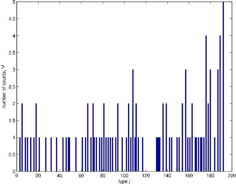
As for the model described in Section 2.2 one can reverse time and employ an backward sampling forward weighting importance sampling method; see [14] for the particular implementation details. In our example we generated data with , and . This is quite a challenging set-up. As in the previous example we set the mutation matrix to be known and uniform and we will concentrate on inferring the . Independent gamma priors with shape and scale parameters equal to were adopted for each of the parameters.
5.2.1 Numerical results
We implemented PMMH using and a simple adaptive scheme for . We allow and use approximately equal spacing between the levels. We choose each with probability proportional to The proposals for the parameters were Gaussian random-walks on the log-scale. The algorithm was implemented in C/C++ was run for iterations, which took approximately 3, 6 and 12 hours to complete. Whilst the run-time is quite long it can be improved by at least one order of magnitude if the SMC is implemented on Graphical Processing Units (GPU) as in [25].
For the dataset plotted in Figure 4 (left) the results are plotted in Figures 4 (right) and 5. The auto-correlation and trace plots indicate that the sampler mixes reasonably well for every . These results in this example are encouraging as to the best of our knowledge Bayesian inference has not been attempted for this class of problems. We expect that practitioners with insight in the field of population genetics can come with more sophisticated MCMC proposals or adaptive schemes for the level sets, so that the methodology can be extended to realistic applications.


6 Discussion
In this article we have presented a multi-level PMCMC algorithm which allows one to perform Bayesian inference for the parameters of a latent stopped processes. In terms of methodology the main novelty of the approach is that uses auxiliary variables to adaptively compute the level sets with . The general structure of this auxiliary variable allows it to incorporate the use of independent SMC runs with less particles to set the levels. In the numerical examples we demonstrated that the addition auxiliary variables slow down the convergence of PMCMC, but this seemed a reasonable compromise in terms of performance compared when fixed number of level sets were used. The proposed algorithm requires considerable amount of computation, but to the authors best knowledge for such problems there seems to be a lack of alternative approaches. Also, recent developments GPU hardware can be adopted to speed up the computations even by orders of magnitude as in [25].
There are several extensions to the work here, which may be considered. Firstly, the scheme that is used to adapt the level sets relies mainly on intuition. We found simple adaptive implementations to work well in practice. In the rare events literature one may find more systematic techniques to design the level sets, based upon optimal control [13] or simulation [9]. Although these methods are not examined here, they can be characterised using alternative auxiliary variables similar to the ones in Proposition 4.3, so the auxiliary variable framework we use is quite generic. In addition, we emphasise that within a PMCMC framework one may also include multi-level splitting algorithms instead of SMC, which might appeal practitioners familiar with multi-level splitting.
Secondly, one could seek to use these ideas within a SMC sampler framework of [16] as done in [12]. As noted in the latter article, a sequential formulation can improve the sampling scheme, sometimes at a computational complexity that is the same as the original PMCMC algorithm. In addition, this article focuses on the PMMH algorithm, so clearly extensions using particle Gibbs and block updates might prove valuable for many applications.
Finally, from a modelling perspective, it may be of interest to apply our methodology in the context of hidden Markov models. In this context, one has
with being the conditional likelihood of the observations. It would be important to understand, given a range of real applications, the feasibility of statistical inference, combined with the development of our methodology. An investigation of the effectiveness of such a scheme when applied to queuing networks is currently underway.
Acknowledgement
We thank Arnaud Doucet and Maria De Iorio for many conversations on this work. The first author was supported by a Ministry of Education grant. The second author was kindly supported by the EPSRC programme grant on Control For Energy and Sustainability EP/G066477/1. Much of this work was completed when the first author was employed by the Department of Mathematics, Imperial College London.
Appendix
Proof.
[Proof of Proposition 4.1] The result is a straight forward application of Theorem 6 of [29] which adapted to our notation states:
where the conditional expectation is the expectation w.r.t. the SMC algorithm (i.e. ) and the outer expectation is w.r.t. the PIMH target (i.e. ). We also denote the estimate of the normalizing constant as with denoting which random variables generate the estimate.
Now, clearly via (A(A1))
with the convention that . Thus, it follows that
and we obtain:
Note that by assumption and thus we have
Given [15, Theorem 7.4.2, Equation (7.17), page 239] and the fact that is defined to be strictly positive in (A(A1)) we have that the SMC approximation is an unbiased estimate of the normalizing constant
| (13) |
and we can easily conclude. ∎
Proof.
[Proof of Proposition 4.2] The proof of parts 1. and 2. follows the line of arguments used in Theorem 4 of [1], which we will adapt to our set-up. The main difference lies in the multi-level construction and second statement regarding the marginal of . For the validity of the multi-level set-up we will rely on Proposition 3.1.
Suppose we design a Metropolis Hastings kernel with invariant density and use a proposal . Then
where we denote the normalising constant of the posterior in (1) as:
Therefore the Metropolis-Hastings procedure to sample from will be as in Algorithm 4.
Alternatively using similar arguments one we may write
Summing over and using the unbiased property of the SMC algorithm in Equation (13) it follows that admits as a marginal, so the proof of part 1. is complete.
∎
Proof.
[Proof of Proposition 4.3] The proof is the similar as that of Proposition 4.2. For the proof of the first statement of part 1. one repeats the same arguments as for Proposition 4.2 with difference being in the inclusion of for and . For the second statement, to get the marginal of , re-write the target as:
Let denote the marginal of obtained in Proposition 4.2. Using (11) and the conditional independence of and , then for the marginal of w.r.t , , we have that
where the summing over and integrating w.r.t. is as in Proposition 4.2.
References
- [1] Andrieu, C., Doucet, A. & Holenstein, R. (2010). Particle Markov chain Monte Carlo methods (with discussion). J. R. Statist. Soc. Ser. B, 72, 269–342.
- [2] Andrieu, C., Doucet, A. & Tadic, V. (2009). On-line parameter estimation in general state-space models using pseudo-likelihood. Technical Report, University of Bristol.
- [3] Andrieu, C. & Roberts, G.O. (2009). The pseudo-marginal approach for efficient Monte Carlo computations. Ann. Statist, 37, 697–725.
- [4] Bahlo, M. & Griffiths, R. C. (2000). Coalescence time for two genes from a subdivided population. J. Math. Biol, 43, 397–410.
- [5] Bibbona, E. & Ditlevsen, S. (2010). Estimation in discretely observed Markov processes killed at a threshold. Technical Report, University of Torino, arXiv:1011.1356v1.
- [6] Blom, H.A.P., Bakker, G.J. & Krystul, J. (2007) Probabilistic Reachability Analysis for Large Scale Stochastic Hybrid Systems. In Proc. 46th IEEE Conf. Dec. Contr., New Orleans, USA.
- [7] Casella, B.& Roberts, G.O. (2008). Exact Monte Carlo simulation of killed diffusions. Adv. Appl. Probab., 40, 273–291.
- [8] Cerou, F. & Guyader, A. (2007). Adaptive multilevel splitting for rare-events analysis. Stoch. Anal. Appl., 25, 417–433.
- [9] Cerou, F., Del Moral, P., FURON, T. & Guyader, A. (2011). Rare event simulation for a static distribution, Stat. Comput., to appear.
- [10] Cerou, F., Del Moral, P. & Guyader, A. (2011). A non asymptotic variance theorem for unnormalized Feynman-Kac particle models. Ann. Inst. Henri Poincare, (to appear).
- [11] Chen, Y., Xie, J. & Liu, J.S. (2005). Stopping-time resampling for sequential Monte Carlo methods. J. R. Statist. Soc. Ser. B, 67, 199–217.
- [12] Chopin, N., Jacob, P. & Papaspiliopoulos, O. (2011). SM: A sequential Monte Carlo algorithm with particle Markov chain Monte Carlo updates. Technical Report, ENSAE, arXiv:1101.1528v2.
- [13] Dean, T. & Dupuis, P. (2009). Splitting for rare event simulation: A large deviations approach to design and analysis. Stoch. Proc. Appl., 119, 562–587.
- [14] De Iorio, M. & Griffiths, R. C. (2004). Importance sampling on coalescent histories. II: Subdivided population models. Adv. Appl. Probab. 36, 434–454.
- [15] Del Moral, P. (2004). Feynman-Kac Formulae: Genealogical and Interacting Particle Systems with Applications. Springer: New York.
- [16] Del Moral, P., Doucet, A. & Jasra, A. (2006). Sequential Monte Carlo samplers. J. R. Statist. Soc. B, 68, 411–436.
- [17] Del Moral, P. & Garnier, J. (2005). Genealogical Particle Analysis of Rare events. Ann. Appl. Prob., 15, 2496–2534.
- [18] Doucet, A., De Freitas, J. F. G. & Gordon, N. J. (2001). Sequential Monte Carlo Methods in Practice. Springer: New York.
- [19] Glasserman, P., Heidelberger, P., Shahabuddin, P. & Zajic, T. (1999). Multilevel splitting for estimating rare event probabilities. Oper. Res., 47, 585–600.
- [20] Gorur, D. & Teh, Y. W. (2009). An efficient sequential Monte-Carlo algorithm for coalescent clustering. Adv. Neur. Infor. Proc. Sys..
- [21] Griffiths, R. C. & Tavare, S. (1994). Simulating probability distributions in the coalescent. Theoret. Pop. Biol., 46, 131–159.
- [22] Johansen, A. M., Del Moral P. & Doucet, A. (2006). Sequential Monte Carlo Samplers for Rare Events, In Proc. 6th Interl. Works. Rare Event Simul., Bamberg, Germany.
- [23] Kantas, N., Doucet, A., Singh, S. S., Maciejowski, J. M. & Chopin, N. (2011). On particle methods for parameter estimation in general state-space models, submitted.
- [24] Kingman, J. F. C. (1982). On the genealogy of large populations. J. Appl. Probab., 19, 27–43.
- [25] LEE, A., YAU, C., GILES, M., Doucet, A. & HOLMES C.C. (2010) On the Utility of Graphics Cards to Perform Massively Parallel Implementation of Advanced Monte Carlo Methods, J. Comp. Graph. Statist., 19, 769–789.
- [26] Lezaud, P., Krystul, J. & Le Gland, F. (2010) Sampling per mode simulation for switching diffusions. In Proc. 8th Internl. Works. Rare-Event Simul. RESIM, Cambridge, UK.
- [27] Liu, J. S. (2001). Monte Carlo Strategies in Scientific Computing. Springer: New York.
- [28] Roberts, G. O. & Rosenthal J. S. (2007). Coupling and ergodicity of adaptive MCMC. J. Appl. Prob., 44, 458–475.
- [29] Roberts, G. O. & Rosenthal J. S. (2011). Quantitative Non-Geometric convergence bounds for independence samplers. Meth. Comp. Appl. Prob., 13, 391–403.
- [30] Sadowsky, J. S. & Bucklew, J. A. (1990). On large deviation theory and asymptotically efficient Monte Carlo estimation. IEEE Trans. Inf. Theor. 36, 579–588.
- [31] Stephens, M. & Donelly, P. (2000). Inference in molecular population genetics (with discussion). J. R. Statist. Soc. Ser. B, 62, 605–655.
- [32] Wilson, I., Weale, M. & Balding, D. J. (2003). Inferences from DNA data: population histories, evolutionary processes and forensic match probabilities. J. R. Statist. Soc. Ser. A, 166, 155–188.
- [33] Whiteley, N. (2010). Discussion of Particle Markov chain Monte Carlo methods. J. R. Statist. Soc. Ser. B, 72, 306–307.