From Majorana Fermions to Topological Order

Kitaev’s well-known toric code [1, 2] is a toy model Hamiltonian which demonstrates the concept of topological order in two dimensions. One can imagine storing a qubit in this ground space of this model such that, at low temperature $T$ compared to the gap, dephasing of such qubit is exponentially suppressed with growing lattice size. More general constructions allow the encoding of many qubits in the ground space and the topological implementation of a cNOT and Hadamard gate by means of Hamiltonian or code deformation [3, 4, 5, 6].

In this paper, we investigate how one could arrive at the toric code Hamiltonian starting from a realistic model of interacting fermions. Kitaev has shown how the toric code emerges in fourth-order perturbation theory from the so-called honeycomb model [8] (see also [9]). Given the recent interest in making proximity-coupled semiconducting nanowires which support weakly-interacting Majorana bound states at their ends [10, 11, 12, 13, 14, 15, 16], we believe that our model may provide a viable route to the realization of topological quantum computation. The interest in Majorana fermion wires is partially motivated by their fermionic-parity protected ground space degeneracy which allows parity protected quantum computation [17, 18, 19] and braiding in networks of nanowires [20, 21, 22, 23]. The advantage of the approach advocated in this paper is that the protection is fully topological and no longer based on fermionic-parity conservation. The idea of engineering a topologically-ordered Hamiltonian using Josephson-junction arrays has been explored mostly in the work of Ioffe et al., see e.g. [25].

We consider the following fermionic Hamiltonian $H=H_{0}+V$ where $H_{0}=\sum_{i}^{2L^{2}}H_{0}^{i}$ and $i$ labels the square islands in Fig. 1. The lattice in Fig. 1(a) has periodic boundary conditions in both directions (see the Appendix for a discussion of the model with open boundaries). Each $H_{0}^{i}$ acts on two fermionic modes or four Majorana modes as

Further, we have $V=\lambda\sum_{i<j}V_{i,j}$ (with $\lambda>0$) where $i,j$ represents the interaction between two Majorana fermions on adjacent islands $i$ and $j$, i.e., $V_{i=\mu\pm\hat{z},j=\mu\pm\hat{x}}$ for a plaquette $\mu$ equals

All link operators $V_{\mu\pm\hat{z},\mu\pm\hat{x}}$ mutually commute. The $\pm$ signs of these terms will be fixed according to the consistent orientation of the plaquettes in Fig. 1, i.e., the link on the top-left of a white plaquette $\mu$ represents the interaction $V_{\mu+\hat{z},\mu-\hat{x}}=ic_{b}^{\mu-\hat{x}}c_{c}^{\mu+\hat{z}}$. Physically, the signs depend on microscopic detail and thus we assume them to be random but fixed. We can find an extensive set of operators which commute with all terms of $H$ and which all mutually commute. These are, first of all, weight-8 fermionic plaquette operators $\{C^{g}_{\mu},C^{w}_{\mu}\}$ (where $g$ ($w$) stands for gray (white) plaquettes $\mu$) which are the product of four link operators around a plaquette:

Secondly, the torus has two homologically non-trivial closed loops $\gamma_{1},\gamma_{2}$ and the loop operators $C_{\gamma_{1/2}}=\Pi_{(i,j)\in\gamma_{1/2}}V_{i,j}$ commute with all link $V_{i,j}$ and island operators $H_{0}^{i}$. Thus the Hamiltonian is block-diagonal with respect to subspaces (‘sectors’) characterized by the eigenvalues $C^{g/w}_{\mu}=\pm 1$ and $C_{\gamma_{1/2}}=\pm 1$.

We analyze the model in the perturbative regime where $\Delta\gg\lambda$, see e.g. [8]. The ground space of $H$ at $\lambda=0$ is characterized by $\{c_{a}^{i}c_{b}^{i}c_{c}^{i}c_{d}^{i}=+1\}$, and thus the ground space on each island is a two-dimensional subspace, a qubit. One can define the logical $X$ and $Z$ operator on this island qubit as

Let $P_{-}=2^{-2L^{2}}\Pi_{i=1}^{2L^{2}}(I+c_{a}^{i}c_{b}^{i}c_{c}^{i}c_{d}^{i})$ be the projector onto this $2^{2L^{2}}$-dimensional unperturbed ground space. The first non-trivial term in the perturbative expansion occurs in $4^{th}$ order (see the Appendix), i.e.

where $A_{\mu}=Z_{\mu+\hat{z}}X_{\mu+\hat{x}}Z_{\mu-\hat{z}}X_{\mu-\hat{x}}$, i.e., the plaquette terms of the toric code in Fig. 2 [28]. Note that $P_{-}C^{g/w}_{\mu}P_{-}=A^{g/w}_{\mu}$ and hence the four-dimensional toric code ground space of $H$ when $\Delta\gg\lambda$ lies in the $\{C^{g/w}_{\mu}=+1\}$ sector.

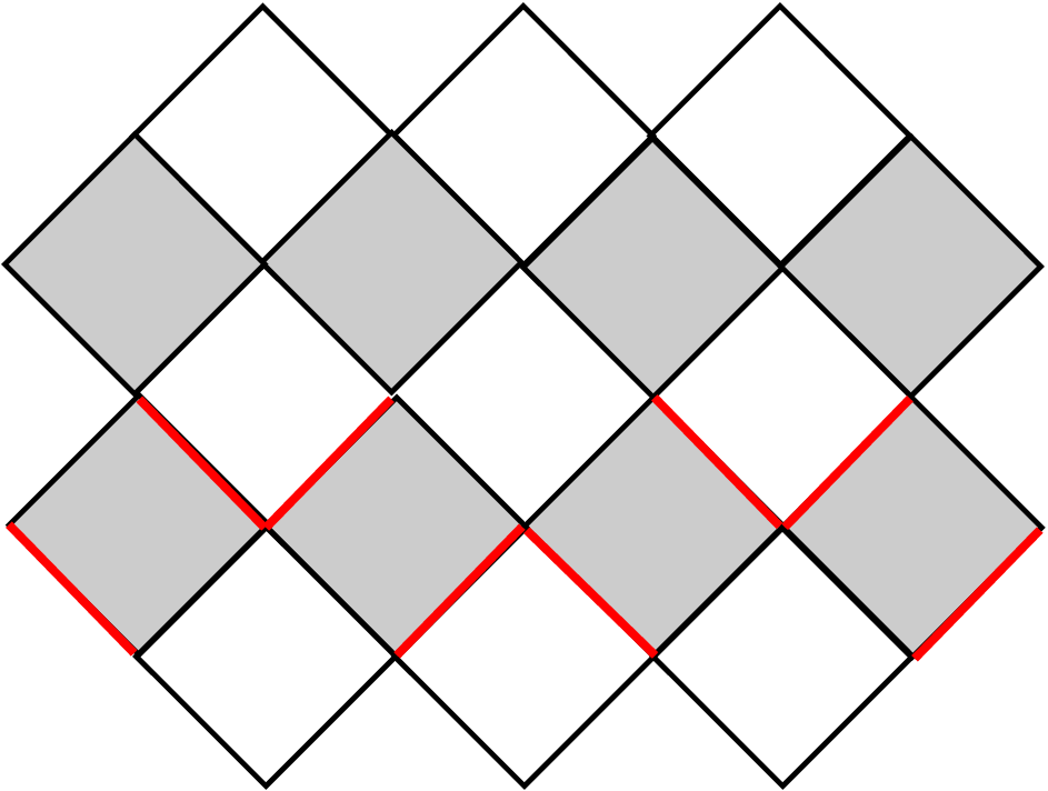
Let us consider how the topological phase extends to the regime where $\frac{\Delta}{\lambda}=O(1)$. We can get insight for this regime by considering higher-order terms in the perturbative expansion (see e.g. [29] for such expansion for the honeycomb model), see the Appendix. This calculation shows that the ground space degeneracy of the toric code is broken only in $(2L)^{\text{th}}$-order perturbation theory and we expect that the topological phase will destabilize via this mechanism.

To consolidate this picture we map our model via a Jordan-Wigner (JW) transformation, onto a family of signed transverse field (TF) Ising models on a 2D square lattice, see Appendix. The JW mapping preserves the locality of the interactions, and all reductions are explicit and rigorous. Previous work [27] has shown how to map an Ising gauge theory in a transverse field (assuming open boundary conditions) by a Jordan-Wigner transformation onto the Majorana fermion model discussed here. Our mapping clarifies the nature of the topological phase transition and the parameter values for which it will occur. In this analysis we restrict ourselves to the sector $\{C^{w}_{\mu}=+1\}$. Note that when $\Delta=0$ the ground state of $H$ is unique since we are in a state of fixed link parity $\{V_{i,j}=-1\}$. This state lies in the $\{C^{g/w}_{\mu}=+1\}$ sector since each $C^{g/w}_{\mu}$ is a product of four link operators. As we saw above, at $\lambda\ll\Delta$, the ground space also lies in the $\{C^{g/w}_{\mu}=+1\}$ sector. The mapping decouples our fermionic model into a set of transverse field Ising models $H(\sigma)=-\lambda\sum_{i,j}\sigma_{i,j}S_{i}^{z}S_{j}^{z}-\Delta\sum_{i}S_{i}^{x}$ with the condition $\Pi_{(i,j)\in\mbox{ \tiny white }\mu}\sigma_{i,j}=1$ so that the sign of the Ising interactions is determined by gauge bits $\sigma_{i,j}\in\{-1,1\}$ associated with the edges. The gauge condition expresses the fact that the white plaquettes are never frustrated, i.e. $C^{w}_{\mu}=+1$, but a gray plaquette is frustrated when $C^{g}_{\mu}=\Pi_{(i,j)\in\mbox{\tiny gray }\mu}\sigma_{i,j}=-1$. The spectrum of $H(\sigma)$ solely depends on the frustration of the Ising interactions and the presence of domain walls or homologically non-trivial loops, see Fig. 3. We anticipate the following spectrum, see Fig. 4. At both ends of the parameter region ($\lambda$ or $\Delta=0$), the groundspace lies in the unfrustrated TF Ising model sector. We have numerically confirmed this for small lattice sizes for the entire parameter regime. Because of the symmetry between gray and white plaquettes, this finding also motivates the choice for $\{C^{w}_{\mu}=+1\}$ as the ground sector. Fig. 3 depicts a configuration $\sigma$ which represents a homologically non-trivial loop; all plaquettes are unfrustrated, but an Ising model with such an AFM sign pattern will contain a domain wall of length at least $L$ where bonds are not satisfied. The topological phase is identified as the paramagnetic (PM) phase $\langle S^{z}\rangle=0$ in the TF Ising models. In this phase the ground spaces of the Hamiltonians $H(\sigma)$ with unfrustrated configurations $\sigma$ with or without the 2 non-trivial AFM loops are approximately degenerate: this is the topological degeneracy whose splitting we expect to scale as $\exp(-L/\xi)$ where $\xi$ is the correlation length of the TF ferromagnetic Ising model. We expect the effective gap $\Delta_{\rm eff}$ above the degenerate ground-space to monotonically increase before we reach the second-order phase transition of the TF ferromagnetic Ising model, which is known to occur around $\left(\frac{\lambda}{\Delta}\right)_{c}\approx 0.33$ [30]. Elementary excitations of the toric code with $A_{\mu}=+1$ for two gray plaquettes $A_{\mu}$ correspond to ground-states of TF Ising models with frustration at those particular gray squares.

We can consider the effect of additional perturbations. One would expect quadratic Majorana fermion perturbations of strength $\epsilon$ on each island due the coupling of the wire ends on an island. If a qubit is encoded in a pair of Majorana wires, such coupling leads to an energy-level splitting of the qubit state of strength $\epsilon$. Here the advantage of our topological encoding becomes clear. Consider a perturbation $U\propto\epsilon\,ic_{b}^{\mu-\hat{x}}c_{d}^{\mu-\hat{x}}$ where $\mu$ is some white plaquette (by symmetry other perturbations would act similarly) and $\epsilon\ll\lambda$. On the groundspace of $H_{0}$, the perturbation acts as a local term $\propto\epsilon X_{\mu-\hat{x}}$, hence we expect that the topological degeneracy is preserved up to some critical strength $(\frac{\epsilon}{\Delta_{\rm eff}})_{c}$ where $\Delta_{\rm eff}$ is the gap above the degenerate ground-space in the topological phase. In practice, we expect these quadratic perturbations to be random (and weak) and hence they could be beneficial in stabilizing the topological quantum memory at finite temperature by limiting the diffusion of anyons (see e.g. [26]).

We analyze the possibility of implementing the model presented above in superconducting-semiconducting heterostructures. Putting a semiconducting nanowire such as InAs or InSb with strong spin-orbit interaction on top of a conventional superconductor subject to a sufficiently strong magnetic field leads to a pair of Majorana modes located at the ends of the nanowire [12, 13]. We focus on a 2D array of superconducting islands each supporting two nanowires leading to four unpaired Majorana modes, see Fig. 1. The product of the four Majorana operators $\mathcal{P}^{i}=c^{i}_{a}c^{i}_{b}c^{i}_{c}c^{i}_{d}$ is fixed by the parity $\mathcal{P}^{i}=(-1)^{n_{i}}$ of the number of electrons $n_{i}$ on the $i$-th island [31, 24]. Two Majorana modes $c^{i}_{x}$ and $c^{j}_{y}$ on different superconducting islands $i$ and $j$ interact with each other via the anomalous Josephson interaction

where $\phi_{i}$ denotes the superconducting phase on the $i$-th island and $\Gamma_{i,j}$ is proportional to the probability amplitude for tunneling a single electron/hole across the link $i,j$ from mode $c^{i}_{x}$ to $c^{j}_{y}$ between the islands $i$ and $j$ [10]. Along the lines of Ref. [22], we shunt each superconducting island with a strong Josephson coupling $E_{J}$ to a common ground superconductor. This Josephson coupling fixes the superconducting phases $\phi_{i}$ to a common value due to large fluctuations of the number of electrons (in units of two) on and off the island. Note that this way of freezing out the bosonic degrees of freedom due to the superconductivity is different from the one discussed in Ref. [24] which proposes a large charging energy which fixes the number of electrons by delocalizing the superconducting phase completely. Even though the charge is strongly fluctuating, the fermion parity $\mathcal{P}^{i}$ remains conserved. In the ideal case when all the Josephson couplings are equal $\Gamma_{i,j}=\lambda$, the anomalous Josephson interaction $H_{J}$ implements $V$. Of course, $V$ in general will not have the orientation indicated in Fig. 1, but if we work with a lattice with open boundary conditions (corresponding to the surface code [32]), any sign pattern of the link interactions simply picks out a topological sector with a corresponding pattern of eigenvalues $A_{\mu}=\pm 1$ as the ground-space [33], see our discussion in the Appendix. From the coding perspective it is well known that topological computation can proceed not just in the trivial syndrome (all eigenvalues of $A_{\mu}=+1$) sector but also in some non-trivial syndrome sector.

Next, we discuss the effect of a capacitive coupling

to the ground plate with the capacitive energy $E_{C}=e^{2}/2C$ where $C$ is the capacitance of the island with respect to ground and $n_{\text{ind}}$ a constant which is due to gate voltages. For simplicity of notation, we have assumed all the capacitances $C$ and offset charges $n_{\text{ind}}$ to be equal. In the regime with $\lambda\lesssim E_{C}\ll E_{J}$, the capacitive coupling introduces phase-slips through the strong Josephson junctions and thus an energy difference between states with different fermion parities. This leads to Eq. (1) with $\Delta\propto E_{C}^{1/4}E_{J}^{3/4}\cos(\pi n_{\text{ind}})e^{-\sqrt{8E_{J}/E_{C}}}$ [22]. The sign of $\Delta$ depends on the value of $n_{\text{ind}}$ can thus be tuned in principle. A residual interaction between two Majorana modes $c^{i}_{x}$ and $c^{i}_{y}$ with strength $\epsilon$ is due to overlap of the wave functions of the Majorana bound states. However, because the states are localized, this coupling can be made exponentially small by keeping the modes sufficiently far apart from each other. Having sufficiently strong tunneling coupling between the Majorana fermions along the links, a value $\lambda\simeq 200\,$mK seem realistic as the bare gap of the Majorana wire is likely of the order of a few K [20]. Choosing the Josephson energy to be $E_{J}\simeq 10\,$K and a capacitive energy $E_{C}\simeq 5\,$K, we obtain $E_{J}\gg\Delta\gtrsim\lambda$ as required . The resulting optimal value of $\Delta_{\text{eff}}$ will be of the order of $\lambda\simeq 200\,$mK.

It is possible to tune the tunnel coupling $\Gamma_{i,j}$ by changing the tunneling barrier between island $i$ and $j$ by a nearby gate. This is a mechanism through which we can create holes in the lattice. In practice one can work with a lattice of superconducting islands which represents the surface code with open boundary conditions, encoding one logical qubit. One can apply the ideas of the surface code architecture if (i) one can make (and move) gray and white holes of arbitrary size in this surface and (ii) one can locally measure $X_{i}$ and $Z_{i}$ and prepare $X_{i}$ and $Z_{i}$ eigenstates. The preparation of certain 1-qubit ancillas can then be used to achieve universality [35]. An example of a white hole qubit is depicted in Fig. 2(b). Such a white hole can be obtained by cutting off the four black links surrrounding the center white plaquette such that the hatched plaquette terms no longer appear in the effective Hamiltonian. Moving such a white hole could be done by adiabatically changing the strength of Majorana links in order to turn links on and off. The operations (ii) can be implemented using the setup of Fig. 1(b). Instead of a single superconducting island, each site consist in fact of two islands with two Majorana modes each. Most of the time, these islands are coupled to each other via a strong Josephson coupling $E_{J}^{\prime}\gg E_{C}^{\prime},E_{C}$ (see Fig. 1) such that they essentially act as a single island such that all the discussion above applies unchanged. Increasing the ratio $E_{C}^{\prime}/E_{J}^{\prime}$ turns on a magnetic field along the $z$-axis which can be used to implement rotations around this axis. Additionally, the measurement of $Z_{i}$ can be implemented by coupling one of the superconducting islands to a fermion parity meter [17]. Single qubit universality is achieved by increasing the overlap of the $a$ and $c$ Majorana modes—by decreasing the length of the topological trivial part of the Majorana wire indicated by the dashed—and thus effectively implementing a magnetic field along the $x$-axis.

We acknowledge fruitful discussions with A. Akhmerov. DDV and FH are grateful for support from the Alexander von Humboldt foundation.

References

- [1] A. Yu. Kitaev, Ann. Phys. (NY) 303, 2 (2003), quant-ph/9707021.
- [2] X.-G. Wen, Phys. Rev. Lett. 90 (1), 016803 (2003).
- [3] E. Dennis, A. Kitaev, A. Landahl, and J. Preskill, J. Math. Phys. 43, 4452 (2002).
- [4] R. Raussendorf, J. Harrington, and K. Goyal, New J. Phys. 9, 199 (2007).
- [5] H. Bombin and M. A. Martin-Delgado, J. Phys. A 42 (9), 095302 (2009).
- [6] A. G. Fowler, A. M. Stephens, and P. Groszkowski, Phys. Rev. A80 (5), 052312 (2009).
- [7] D. P. DiVincenzo, Phys. Scr. T137, 014020 (2009).
- [8] A. Yu. Kitaev, Ann. Phys. (NY) 321, 2 (2006).
- [9] C. G. Brell, S. T. Flammia, S. D. Bartlett, and A. C. Doherty, New J. Phys. 13, 053039 (2011).
- [10] A. Yu. Kitaev, Phys.-Usp. 44 (suppl.), 131 (2001), cond-mat/0010440.
- [11] L. Fu and C. L. Kane, Phys. Rev. Lett. 100, 096407 (2008).
- [12] R. M. Lutchyn, J. D. Sau, and S. Das Sarma, Phys. Rev. Lett. 105, 077001 (2010).
- [13] Y. Oreg, G. Refael, and F. von Oppen, Phys. Rev. Lett. 105, 177002 (2010).
- [14] V. Mourik, K. Zuo, S. M. Frolov, S. R. Plissard, E. P. A. M. Bakkers, and L. P. Kouwenhoven, Science 336, 6084 (2012).
- [15] M. T. Deng, C. L. Yu, G. Y. Huang, M. Larsson, P. Caroff, and H. Q. Xu, arXiv:1204.4130 (2012).
- [16] L. P. Rokhinson, X. Liu, and J. K. Furdyna, arXiv:1204.4212 (2012).
- [17] F. Hassler, A. R. Akhmerov, C.-Y. Hou, and C. W. J. Beenakker, New J. Phys. 12, 125002 (2010); F. Hassler, A. R. Akhmerov, and C. W. J. Beenakker, ibid. 13, 095004 (2011)
- [18] J. D. Sau, R. M. Lutchyn, S. Tewari, and S. Das Sarma, Phys. Rev. Lett. 104, 040502 (2010).
- [19] C. W. J. Beenakker, arXiv:1112.1950 (2011).
- [20] J. Alicea, Y. Oreg, G. Refael, F. von Oppen, and M. P. A. Fisher, Nature Phys. 7, 412 (2011).
- [21] J. D. Sau, D. J. Clarke, and S. Tewari, Phys. Rev. B 84, 094505 (2011).
- [22] B. van Heck, A. R. Akhmerov, F. Hassler, M. Burrello, and C. W. J. Beenakker, New J. Phys. 14, 035019 (2012).
- [23] B. I. Halperin, Y. Oreg, A. Stern, G. Refael, J. Alicea, and F. von Oppen, Phys. Rev. B 85, 144501 (2012).
- [24] C. Xu and L. Fu, Phys. Rev. B 81 (13), 134435 (2010).
- [25] S. Gladchenko et al., Nature Physics 5, 48–53 (2009).
- [26] C. Stark et al., Phys. Rev. Lett. 107, 030504 (2011), J. Wootton and J. Pachos, Phys. Rev. Lett. 107, 030504 (2011).
- [27] E. Fradkin, M. Srednicki and L. Susskind, Phys. Rev. D 21, 2885-2891 (1980).
- [28] The more familiar representation of the toric code is obtained by unitarily rotating on all qubits which are at positions for, say, the gray plaquettes.
- [29] J. Vidal, K.P. Schmidt, S. Dusuel, Phys. Rev. B 78, 245121 (2008).
- [30] A. D. B. K. Chakrabarti and P. Sen, Quantum Ising Phases and Transitions in Transverse Ising Models (Springer, 1996).
- [31] L. Fu, Phys. Rev. Lett. 104, 056402 (2010).
- [32] S. B. Bravyi and A. Yu. Kitaev, Quantum codes on a lattice with boundary, quant-ph/9811052 (1998).
- [33] This is not true for the toric code in which plaquette operators are linearly dependent and a flipped sign of a link can lead to frustration.
- [34] J. Koch, T. M. Yu, J. Gambetta, A. A. Houck, D. I. Schuster, J. Majer, A. Blais, M. H. Devoret, S. M. Girvin, and R. J. Schoelkopf, Phys. Rev. A 76, 042319 (2007).
- [35] S. Bravyi and A. Yu. Kitaev, Phys. Rev. A 71, 022316 (2005).
- [36] F. L. Pedrocchi, S. Chesi, and D. Loss, Phys. Rev. B 84 (16), 165414 (2011).
- [37] E. H. Lieb, Phys. Rev. Lett. 73, 2158 (1994).
- [38] This procedure is similar to Kitaev’s analysis of the honeycomb model [8] where one obtains a noninteracting fermion model only if we consider an extended space of states, see also the discussion in [36].
- [39] Perhaps one can prove this with techniques similar as in Ref. [37]. In this case we have a family of spin Hamiltonians (not fermionic) on a square-octagon lattice which depend on the parameters and one wishes to prove that the state of minimal energy is obtained when .