TripNet: A Heuristic Algorithm for Constructing Rooted Phylogenetic Networks from Triplets

Phylogenetic networks are a generalization of phylogenetic trees that permit the representation of non-tree-like underlying histories. A rooted phylogenetic network is a rooted directed acyclic graph in which no nodes has indegree greater than 2 and the outdegree of each node with indegree 2 is 1. Such nodes are called reticulation nodes. Mathematicians are interested in developing methods that infer a phylogenetic tree or network from basic building blocks. In the computation of a rooted tree or network, one group of the basic building blocks are triplets, the rooted binary trees on three taxa [1]. In 1981, Aho et al., studied the problem of constructing a tree from a set of triplets [2]. They proposed an algorithm called the BUILD algorithm which shows that, given a set of triplets, it is possible to construct in polynomial time a rooted tree that all the input triplets are contained in it or decide that no such tree exists. When there is no tree for a given set of triplets one may try to produce an optimal phylogenetic network. In this context, the goal is to compute an optimal rooted phylogenetic network that contains all the rooted triplets. One possible optimality criterion is to minimize the level of the network, which is defined as the maximum number of reticulation nodes contained in any biconnected component of the network. The other optimality criterion is to minimize the number of reticulation nodes [1]. In [3] and [4] the authors considered the problem of deciding whether, given a set of triplets as input, is it possible to construct a level-1 phylogenetic network that contains all the input triplets? They showed that, in general, this problem is NP-hard. However, in [4] the authors showed that when the set of triplets is dense, which means that for each set of three taxa there is at least one triplet in the input set, the problem can be solved in polynomial time. After their results, all research in this new area has up to this point focused on constructing networks from dense triplet sets. The algorithm by [5] can be used to find a level-1 or a level-2 phylogenetic network which minimizes the number of reticulation nodes if such a network exists. In [6] the authors showed that given a dense set of triplets $\tau$ and a fixed number $k$, it is possible to construct in time $O(|\tau|^{k+1})$ a level-$k$ phylogenetic network consistent with $\tau$ or decides that no such network exists.

In this paper we present a heuristic algorithm called TripNet for constructing phylogenetic networks from an arbitrary set of triplets. Despite of current methods that work for dense set of triplets, a key innovation is the applicability of TripNet to non-dense set of triplets. The results of the TripNet algorithm on biological sequences is presented in [7]. Here we prove some theorems to justify the performance of the algorithm. This paper is organized as follows. In section II we present some definitions and notation. In section III we discuss triplet construction methods. In section IV the directed graph $G_{\tau}$ related to a set of triplets $\tau$ is introduced. In section V the concept of the height function of a tree is introduced, and we propose an algorithm to construct a tree from its height function. Then we generalize the concept of the height function to the networks. Finally, in section VI we present the TripNet algorithm.

Let $X$ be a set of taxa. A rooted phylogenetic tree (tree for short) on $X$ is a rooted unordered leaf labeled tree whose leaves are distinctly labeled by $X$ and every node which is not a leaf has at least outdegree two. A directed acyclic graph (DAG) is a directed graph that is free of directed cycles. A directed acyclic graph $G$ is connected if there is an undirected path between any two nodes of $G$. It is biconnected if it contains no node whose removal disconnects $G$. A biconnected component of a graph $G$ is a maximal biconnected subgraph of $G$. A rooted phylogenetic network (network for short) on $X$ is a rooted directed acyclic graph in which root has indegree 0 and outdegree 2 and every node except the root satisfies one of the following conditions:
a) It has indegree 2 and outdegree 1. These nodes are called reticulation nodes.
b) It has indegree 1 and outdegree 2.
c) It has indegree 1 and outdegree 0. These nodes are called leaves and are distinctly labeled by $X$.

A reticulation leaf is a leaf whose parent is a reticulation node. A network is said to be a level-$k$ network if each of its biconnected component contains at most $k$ reticulation nodes. A tree can be considered as a level-0 network.

A rooted triplet (triplet for short) is a binary rooted unordered tree with three leaves. We use $ij|k$ to denote the triplet with taxa $i$ and $j$ on one side and $k$ on the other side of the root (Fig.??). A set of triplets $\tau$ is called dense if for each subset of three taxa, there is at least one triplet in $\tau$. A triplet $ij|k$ is consistent with a network $N$ or equivalently $N$ is consistent with $ij|k$ if $N$ contains a subdivision of $ij|k$, i.e. if $N$ contains distinct nodes $u$ and $v$ and pairwise internally node-disjoint paths $u\rightarrow i$, $u\rightarrow j$, $v\rightarrow u$ and $v\rightarrow k$. Fig. ?? shows an example of a network which is consistent with $ij|k$. A set $\tau$ of triplets is consistent with a network $N$ if all the triplets in $\tau$ are consistent with $N$. We use the symbols $\tau(N)$ and $L_{N}$ to represent the set of all triplets that are consistent with $N$ and the set of labels of its leaves respectively. For any set $\tau$ of triplets define $L(\tau)=\cup_{t\in\tau}{L_{t}}$. The set $\tau$ is called a set of triplets on $X$ if $L(\tau)=X$.

There are two main tree construction methods, character-based methods and distance-based methods. In character-based methods, the information of a set $X$ of biological sequences is directly used for producing final tree. In distance-based methods first a distance matrix $D$ is computed from $X$ and then a rooted (or unrooted) tree $T$ is constructed from $D$ [1].

A weighted tree $(T,w)$ is a rooted (or unrooted) tree $T$ together with a function $w:E(T)\rightarrow\mathbb{R}$. We call $w(e)$ the weight of the edge $e$. For any two nodes $i$ and $j$ of $T$, let $l_{ij}$ denotes the unique path in $T$ from $i$ to $j$. Define

If $T$ is an unweighted tree then we suppose that for each edge $e$ in $T$, $w(e)=1$. Given a set of taxa $X$, let $(T,w)$ be a weighted tree on $X$ and $D_{T}$ be a matrix in which the entry of row $i$ and column $j$ is $d_{T}(i,j)$. We call $D_{T}$ the distance matrix related to $(T,w)$.

A quartet is a binary unrooted tree with four leaves. We use the symbol $ij|kl$ for a quartet on the set of taxa $\{i,j,k,l\}$ which have neighbor pairs $i,j$ and $k,l$. In a quartet $Q$ there is a unique edge such that its two end points are not leaves. We call this edge the inner edge of $Q$ $($ Fig. ?? $)$. A weighted quartet is called $informative$, if the weight of its inner edge is positive. The following proposition holds for informative quartets.

The following proposition also holds [9].

Suppose that $X$ is a set of taxa in which each taxon is a biological sequence. Let $o_{X}$ be an outgroup for $X$ and $D$ be a distance matrix on $X\cup\{o_{X}\}$. In this paper to obtain a set of triplets, we use the method introduced in [5]. For each set of four taxa that contains $o_{X}$, we construct the unique quartet which satisfies Proposition ??. Then, by removing $o_{X}$ from informative quartets we obtain the set of triplets. In the rest of paper we refer to this method By QOT.

Let $\tau$ be a set of triplets. Define $G_{\tau}$, the directed graph related to $\tau$, by $V(G_{\tau})=\{~\{i,j\}:i,j\in L(\tau),i\neq j\}$ (we denote $\{i,j\}$ by $ij$ for short) and $E(G_{\tau})=\{(ij,ik):ij|k\in\tau\}\cup\{(ij,jk):ij|k\in\tau\}$. The graph $G_{\tau}$ has an important role in the remaining of the paper and in this section we prove some basic properties of $G_{\tau}$.

Let $X$ be a set of sequences, $D=[d(i,j)]$ be a distance matrix on $X$ where for any pair $i,j\in X$, $d(i,j)$ denotes the distance between them, and $\tau$ be the set of triplets that is produced by QOT method. Here we define the concept of the closure of $\tau$. If $ij|k$ and $js|i$ are in $\tau$, then we have the quartets $ij|ko_{X}$ and $js|io_{X}$. According to the Proposition ??, $d(i,j)+d(k,o_{X})<d(j,k)+d(i,o_{X})$, $d(j,s)+d(i,o_{X})<d(i,j)+d(s,o_{X})$, and therefore $d(j,s)+d(k,o_{X})<d(j,k)+d(s,o_{X})$. It means that we should have the quartet $js|ko_{X}$. The equivalent triplet for this informative quartet is $js|k$. If this triplet is not in $\tau$ add it to $\tau$ and continue this procedure until one cannot add more triplets. We use the symbol $\overline{\tau}$ to show this new set of triplets and call it the closure of $\tau$.

The following lemma is an immediate consequence of the definition of $\overline{\tau}$.

Now we state the main results of this section.

Let $\tau$ be a set of triplets that is consistent with a tree. Let $T_{\tau}$ denotes the unique tree that is produced by the BUILD algorithm.

In this section first the concept of the height function of a tree and a DAG is introduced and then the BUILD algorithm is restated based on this concept.

Let $X\choose 2$ denotes the set of all subsets of $X$ of size $2$.

Let $T$ be a rooted tree with the root $r$, $c_{ij}$ be the lowest common ancestor of the leaves $i$ and $j$, and $l_{T}$ denotes the length of the longest path started from $r$.

The following theorem represents the relation between the height function of a tree and a triplet consistent with it.

Let $\tau$ be a set of triplets, $G_{\tau}$ be a DAG and $l_{G_{\tau}}$ denotes the length of the longest path in $G_{\tau}$. Since $G_{\tau}$ is a DAG, the set of nodes with outdegree zero is nonempty. Assign $l_{G_{\tau}}+1$ to the nodes with outdegree zero and remove them from $G_{\tau}$. Assign $l_{G_{\tau}}$ to the nodes with outdegree zero in the resulting graph and continue this procedure until all nodes are removed.

Let $\tau$ be a set of triplets that is consistent with a tree. By Theorem ??, $G_{\tau}$ is a DAG and $h_{G_{\tau}}$ is well-defined. The following theorem represents a method to obtain $h_{{T}_{\tau}}$ from $\tau$ using $h_{G_{\tau}}$.

Now we describe an algorithm similar to BUILD algorithm, using height function. We refer to this algorithm by HBUILD. Let $h$ be a height function on $X$. Define a weighted complete graph $(G,h)$ where $V(G)=X$ and edge $\{i,j\}$ has weight $h(i,j)$. Remove the edges with maximum weight from $G$. If removing these edges results a connected graph the algorithm stops. Otherwise, the process of removing the edges with maximum weight is continued in each connected component until each connected component contains only one node. At the end of this procedure one can reconstruct the tree by reversing the steps of the algorithm similar to BUILD algorithm (see Fig. 2). The algorithm above decides in polynomial time whether a tree with height function $h$ exists.

Now if $\tau$ is a set of triplets which is consistent with a tree, by Theorems ?? and ??, $G_{\tau}$ is a DAG and $h_{G_{\tau}}=h_{T_{\tau}}=h$ and HBUILD algorithm constructs $T_{\tau}$.

Now we generalize the concept of height function from trees to networks. This generalization is not straightforward because the concept of (lowest) common ancestor of two leaves of a network is not well-defined. Let $N$ be a network with the root $r$ and $l_{N}$ be the length of the longest directed path from $r$ to the leaves. For each node $u$ consider $d(u,r)$ as the length of the longest directed path from $r$ to $u$. For any two nodes $u$ and $v$, we call $u$ an ancestor of $v$, if there exists a directed path from $u$ to $v$. If $u$ is an ancestor of $v$ then we say that $v$ is lower than $u$. Lowest common ancestor of two leaves in a network is not necessarily unique. For any two leaves $i$ and $j$, let $C_{ij}$ be the set of all lowest common ancestors of $i$ and $j$.

Obviously, every network $N$ indicates a unique height function $h_{N}$. But two different networks may have the same height function (see Fig. ??) .

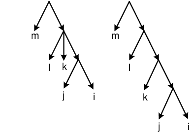
In the following proposition we prove that for a given height function $h$ there is a network $N$ such that $h_{N}=h$.

The following theorem shows the relation between height function of a network and the triplet consistency with it.

The reverse of the above theorem is not necessarily true. For example, consider the network of Fig. ?? . The triplet $ij|k$ is consistent with it, but $h(i,j)=h(i,k)=3$ and $h(j,k)=2$.

The basic idea of the TripNet algorithm is to find a height function as an intermediate computational step that yields the minimum amount of information required to construct the network from a set of triplets. So it is important to find a way for computing $h_{N}$ from a set of triplets. In the rest of this section we introduce a computational method for computing $h_{N}$ using Integer Programming. Let $\tau$ be a set of triplets with $|L(\tau)|=n$. Inspiring from Theorems ?? and ??, for each triplet $ij|k\in\tau$, define two inequalities $h(i,k)-h(i,j)\geq 1$ and $h(j,k)-h(i,j)\geq 1$. Since the number of variables in such inequalities are at most $c(n,2)$, we obtain the following system of inequalities from $\tau$.

Let $s$ be an integer. Define the following Integer Programming and call it IP($\tau,s$).

Intuitively if IP($\tau,s$) has a feasible solution, we expect that the optimal solution to this integer programming is an approximation of the height function of an optimal network $N$ consistent with $\tau$. The following theorems support this intuition.

Let $\tau$ be a set of triplets consistent with a tree. By Theorems ??, ??, and ??, $h_{T_{\tau}}$ is a feasible solution to IP($\tau,l_{G_{\tau}}+1$). In the following theorem we prove the uniqueness of this solution.

The BUILD tree is not necessarily a binary tree. To obtain a binary tree consistent with a set of triplets we do the following procedure.

Let $T$ be a tree and $x$ be a node of $T$ with $x_{1},x_{2},\ldots,x_{k}$, $k\geq 3$ as its childs. Consider a new node $y$. Construct $T^{\prime}$ by removing the edges $(x,x_{1}),(x,x_{2}),\ldots,(x,x_{k-1})$ from $T$ and adding the edges $(x,y),(y,x_{1}),(y,x_{2}),\ldots,(y,x_{k-1})$ to $T$. Continuing the same method for each node with outdegree more than 2 we obtain a binary tree which we call it a binarization of $T$ (see Fig. ??). Obviously, we can obtain different binarization of $T$. The proof of the following theorem is easy and we omit it.

Now we describe the TripNet algorithm in nine steps. In this algorithm the input is a set of triplets $\tau$ and the output is a network consistent with $\tau$. Also if $\tau$ is consistent with a tree the algorithm constructs a binarization of $T_{\tau}$.

Step 1: In this step we find a height function $h$ on $L(\tau)$. If $G_{\tau}$ is a DAG we set $G^{\prime}_{\tau}=G_{\tau}$. If $G_{\tau}$ is not a DAG we remove some edges from $G_{\tau}$ in such a way that the resulting graph $G^{\prime}_{\tau}$ is a DAG. Set $h=h_{G^{\prime}_{\tau}}$.

If $\tau$ is obtained from biological sequences using the QOT method, then Theorems ?? shows that $G_{\tau}$ is a DAG. Removing minimum number of edges from a directed graph to make it a DAG is known as the minimum Feedback Arc Set problem which is NP-hard [10]. Thus, using a greedy algorithm, we try to remove as minimum number of edges as possible from $G_{\tau}$ in order to lose minimum information. However, any such missing information will be recaptured in Step 9.

Step 2: In this step TripNet first apply HBUILD on $h$. If the result is a tree, TripNet constructs a binarization of this tree. Otherwise TripNet goes to Step 3.

Note that if $\tau$ is consistent with a tree, by Theorem ??, $h_{G_{\tau}}=h_{T_{\tau}}$ and TripNet constructs a binarization of $T_{\tau}$.

Step 3: Remove all the maximum-weight edges from $G$. The process of removing all the maximum-weight edges from the graph continues until the resulting graph is disconnected.

In [3] and [4] the authors introduced the concept of $SN$-sets for a set of triplets $\tau$. A subset $S$ of $L(\tau)$ is an $SN$-set if there is no triplet $ij|k\in\tau$ such that $i\notin S$ and $j,k\in S$. In [4] it is shown that if $\tau$ is dense then the maximal $SN$-sets partition $L(\tau)$ and can be found in polynomial time. By contracting each of the $SN$-set to a single node and assuming a common ancestor for all of these leaves, the size of the problem is reduced. In these papers, for finding the maximal $SN$-sets in polynomial time, the authors use the high density of the input triplet sets. TripNet algorithm uses the concept of height function as an auxiliary tool to obtain $SN$-sets instead of the high density assumption.

Step 4: For each connceted component obtaining in Step 3, which is not an $SN$-set we apply Step 3. This process continues until all of the resulting components are $SN$-sets. Let $\{S_{1},S_{2},\ldots,S_{k}\}$ be the set of resulting $SN$-sets. If each $SN$-set contains only one node, HBUILD is applied and if the result is a tree TripNet constructs a binary tree and goes to Step 6. Otherwise TripNet goes to Step 5. If for some $i$, $|S_{i}|>1$, contract each $S_{i}$ to a single node $s_{i}$ and set $S=\{s_{1},s_{2},\ldots,s_{k}\}$. Update the set of triplets by defining $\tau_{S}=\{s_{i}s_{j}|s_{k}:if~\exists~xy|z\in\tau,~x\in S_{i},~y\in S_{j}~$ and $~z\in S_{k}\}$. Constructs a weighted complete graph $(G_{S},w_{S})$ with $V(G_{S})=S$ and $w_{S}(s_{i},s_{j})=\min\{h(x,y):x\in S_{i}~and~y\in S_{j}\}$. Set $(G,w)=(G_{S},w_{S})$ and TripNet goes to Step 3.

The following theorem is consequence of definition $SN$-set for $(G_{S},w_{S})$.

In the next step the reticulation leaves are recognized using the following three criteria:

Criterion I: Let $m_{i}$ and $M_{i}$ be the minimum and maximum weight of the edges in $(G,h)$ with exactly one end in $S_{i}$. Choose the node with minimum $m_{i}$ and if there is more than one node with minimum $m_{i}$ then choose among them the nodes which has minimum $M_{i}$. Let $R_{1}$ denotes the set of such nodes.

Criterion II: Let $w_{min}=min\{w(s_{i},s_{j}):1\leq i,j\leq k\}$. In $G_{S}$ consider the induced subgraph on the edges with the weight $w_{min}$. Choose the nodes of $R_{1}$ with the maximum degree in this induced subgraph. Let $R_{2}$ denotes the set of such nodes.

References

- (1) D.H. Huson, R. Rupp and C. Scornavacca, Phylogenetic Networks Concepts, Algorithms and Applications, Cmbridge University Press, 2010.
- (2) A.V. Aho, Y. Sagiv, T.G. Szymanski and J.D. Ullman, ”Inferring a tree from lowest common ancestors with an application to the optimization of relational expressions,” SIAM J. Comp., vol. 10, pp. 405-421, 1981.
- (3) J. Jansson, N.B. Nguyen and W.K. Sung, ”Algorithms for combining rooted triplets into a galled phylogenetic network,” Proc. Sixteenth annual ACM-SIAM symposium on Discrete algorithms, vol. 24, pp. 23-25, 2007.
- (4) J. Jansson and W.K. Sung, ”Inferring a Level-1 Phylogenetic Network from a Dense Set of Rooted Triplets,” Theoretical Computer Science, vol. 363, pp. 60-68 , 2006.
- (5) L.V. Iersel and S. Kelk, ”Constructing the Simplest Possible Phylogenetic Network from Triplets,” Algorithmica, 2009.
- (6) T.H. To and M. Habib, ”Level-k Phylogenetic Network can be Constructed from a Dense Triplet Set in Polynomial Time,” In CPM 2009, pp. 275-288, 2009.
- (7) R. Tusserkani, Ch. Eslahchi, H. Poormohammadi and A. Azadi, ”TripNet: A Method for Constructing Phylogenetic Networks from Triplets,” arXiv:1104.4720v1, 2011.
- (8) L.V. Iersel, J. Keijsper, S. Kelk, L. Stougie, F. Hagen and T. Boekhout, ”Constructing level-2 phylogenetic networks from triplets,” In RECOM 2008, vol. 4955, pp. 450-462, 2008.
- (9) H-J. Bandelt and M.A Steel, ”Symmetric matrices representable by weighted trees over a cancellative abelian monoid,” SIAM, J. Disc. Math, vol. 8, No. 4, pp 517-525, 1995.
- (10) R. Karp, ”Reducibility among combinatorial problems,” Proc. Sympos., IBM Thomas J. Watson Res. Center, Yorktown Heights, N.Y., pp. 85-103, 1972.