Energy Efficient Iterative Waterfilling for the MIMO Broadcasting ChannelsThanks: This work is supported in part by Huawei Technologies, Co. Ltd., Shanghai, China and National Basic Research Program of China (973 Program) 2007CB310602.Thanks: Corresponding author: Ling Qiu, lqiu@ustc.edu.cn.
Abstract
Optimizing energy efficiency (EE) for the MIMO broadcasting channels (BC) is considered in this paper, where a practical power model is taken into account. Although the EE of the MIMO BC is non-concave, we reformulate it as a quasiconcave function based on the uplink-downlink duality. After that, an energy efficient iterative waterfilling scheme is proposed based on the block-coordinate ascent algorithm to obtain the optimal transmission policy efficiently, and the solution is proved to be convergent. Through simulations, we validate the efficiency of the proposed scheme and discuss the system parameters’ effect on the EE.
Index Terms:
Energy efficiency, MIMO broadcasting channels, iterative waterfilling.I Introduction
Wireless communication turns to the era of green. This is not only because of the exponential traffic growth with the popularity of the smart phone but also the limited energy source with ever higher prices. Energy efficiency (EE), as a result, becomes one of the major topics in the research of wireless communications [1] and plenty of research projects either government funded or industrial funded start to investigate the energy efficient solutions for the wireless network as well as the sustainable future for the wireless communications. Meanwhile, multiple input multiple output (MIMO), especially downlink multiuser MIMO (also called MIMO broadcasting channels, BC), has become a key technology in the cellular networks due to its significant spectral efficiency (SE) improvement. Therefore, studying the EE of the MIMO BC is a critical issue.
The EE is in general defined as the capacity divided by the power consumption, which denotes the delivered bits per-unit energy measured in bits per-Joule. There are a lot of literatures discussing the EE of the point to point MIMO channels [2, 3, 4, 5, 6, 7]. The point to point MIMO channels can always be separated into parallel sub-channels through singular value decomposition (SVD) or after detection. In this case, only power allocation across the sub-channels needs to be optimized to compromise the transmit power and circuit power, and thus maximize the EE [3, 4, 5]. As the sub-channels are parallel, the solution is similar with the energy efficient power allocation in OFDM systems [8, 9]. The optimization for point to point MIMO channels is not applicable for the MIMO BC, as the MIMO BC cannot be simply transformed into parallel sub-channels11 1 Although after zero-forcing (ZF) precoding, for example, the MIMO can be separated into parallel sub-channels, the ZF scheme is far away from the optimal solution [10].. There are few literatures discussing the EE for the MIMO BC. To the best of the authors’ knowledge, only [11] and our previous work [12] addressed this topic, but they both assumed linear precoding design and equal transmit power allocation for simplification. The assumption of linear precoding makes both works far away from the optimal solution. To optimize the system performance (both SE and EE) of the MIMO BC, the precoding matrices and power allocation should be jointly decided. For instance, the common way to achieve the maximum sum capacity is employing the dirty paper coding (DPC) and iterative waterfilling [10, 13, 14, 15]. From the standpoint of EE, joint precoding and power allocation design should also be carefully designed to achieve the optimum, which is the main concern of this paper.
We consider the problem of optimizing EE with joint precoding and power allocation for the MIMO BC, where a practical power model including signal processing, circuit power, etc. at the base station (BS) [12, 16] is taken into account. After formulating the maximum EE problem, we find that the energy efficient joint precoding and power allocation design is equivalent to only optimizing the transmit covariance matrices. However, optimizing the transmit covariance matrices is difficult, as the EE function achieved by DPC is nonconcave. Fortunately, we find an efficient iterative solution based on uplink-downlink duality and the contributions are summarized as follows.
Contributions: We transform the EE into a quasiconcave function through employing the famous uplink-downlink duality. The duality transforms the nonconcave MIMO BC capacity into the dual convex MIMO multi-access channels (MAC). After that, we propose a novel energy efficient iterative waterfilling scheme based on the block-coordinate ascent algorithm to solve the quasiconcave EE optimizing problem efficiently. During each iteration, the transmit covariance matrices optimization is formulated as a concave fractional program, and solved through relating it to a parametric concave program and then applying the Karush-Kuhn-Tucker optimality conditions. Interestingly, the solution of each iteration has a feature of waterfilling. We prove the convergence of the proposed scheme and validates it through simulations. Moreover, the system parameters’ effect on the EE is discussed finally.
II System Model
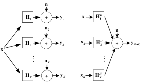
The system consists of a single BS with antennas and users each with antennas22 2 The results here can be extended to the general case with different antenna number at each user. Moreover, the results are also applicable to the multi-cell scenario with BS cooperation., which is shown in Fig. 1. The downlink channel can be denoted as
| (1) |
and the dual uplink channel is denoted as
| (2) |
where is the channel matrix of the th user, is the transmitted signal on the downlink, is the transmitted signal on the uplink, and are the independent Gaussian noise with each entry . Frequency flat fading channels with bandwidth is considered and the channel state information (CSI) is assumed to be perfectly known at the transmitter and receivers.
About the power model, as BSs take the main power consumption in the cellular networks, the users’ consumed power is omitted. The BS power model is motivated by [12, 16]. As the power radiated to the environment for signal transmission is only a portion of its total power consumption [16], the practical circuit power, signal processing power, cooling loss etc. at the BS should be taken into account. Without loss of generality, given the total BS antenna number and total transmit power , the total power consumption of a BS can be denoted as
| (3) |
where denotes the power amplifier (PA) efficiency; denotes the dynamic power consumption proportional to the number of radio frequency (RF) chains, e.g. circuit power of RF chains which is always proportional to ; and accounts for the static power independent of both and which includes power consumption of the baseband processing, battery unit etc..
III Achievable Sum Capacity and Energy Efficiency
The sum capacity of the MIMO BC is achieved by DPC, which can be denoted as follows [10] given a total transmit power .
| (4) |
where the optimization is performed to choose the optimal downlink transmit covariance matrices .
The EE is defined as the achievable sum capacity of MIMO BC divided by the total power consumption at the BS, which can be denoted as
| (5) |
under a fixed transmit power . Based on (5), the optimal EE for the MIMO BC can be obtained through optimizing 33 3 Indeed, the EE of MIMO BC is highly affected by the transmit power and transmit antenna number , and jointly optimizing and is required to maximize the EE. We only consider the optimization of in this paper, and the optimizing to further improve the EE based on active transmit antenna selection can be found in [17]., which is denoted as
| (6) |
In the above optimization problem, transmit power level and transmit covariance matrices need to be jointly optimized. Note that although no maximum transmit power constraint is considered in (6), the solution can be easily extended to the constrained case based on [8, 18]. We omit the extension here due to page limit.
As (6) is nonconcave, optimizing (6) is nontrivial. Fortunately, motivated by [19, 20], we find out that the following property. If the numerator (sum capacity) can be transformed into a convex function, the EE can be formulated as a quasiconcave function, because the denominator (total power consumption) is affine. Based on this observation, we try to transform the sum capacity into a concave function.
Applying the uplink-downlink duality [13], the MIMO BC sum capacity (4) is equal to the concave sum capacity of the MIMO MAC (2) with sum transmit power constraint, which can be denoted as
| (7) |
where the uplink transmit covariance matrices need to be optimized. Thus, the dual MAC optimal EE should be rewritten as
| (8) |
According to the duality and the mapping between and [13], optimal and can be obtained if we can get the optimal and in (8). Furthermore, since the maximum power constraint is not considered and is always required for optimizing (7) [14], (8) can be simplified and rewritten as
| (9) |
Finally, the optimization of (6) is transformed into optimizing (9). If we can obtain the optimal for (9), the optimal can be decided correspondingly based on . That is to say, designing the joint precoding and power allocation to maximize EE is equivalent to optimizing the transmit covariance matrices. Once transmit covariance matrices are decided, the transmit power level can be correspondingly determined.
Let us look at (9) again. Since the numerator is concave and the denominator is affine, (9) is a quasiconcave optimization, which can be solved through the bisection method or interior-point methods. However, the numerical methods would be still too complex when the user number becomes significantly large. Motivated by [14, 15], an energy efficient iterative waterfilling is proposed in the next section to solve it more efficiently.
IV Energy Efficient Iterative Optimization
IV-A Motivation
As the EE is distinct from the capacity, the spectral efficient iterative waterfilling [14] is not applicable for the EE any longer. Nevertheless, we notice that the basic idea of the spectral efficient iterative algorithms are based on the block-coordinate ascent algorithm [21, Sec. 2.7]. That is to say, if we can write the EE as the similar structure with the block-coordinate ascent algorithm and then prove it satisfies the condition of [21, Sec. 2.7], we can obtain an iterative solution of the problem (9).
For ease of description, we define the following function at first.
| (10) |
For the block-coordinate ascent algorithm, given the current iterate , the next iterate can be generated as
| (11) |
However, to apply the iterative algorithm efficiently, there are conditions need to be satisfied. For one thing, the solution of (11) should be uniquely attained [21, Proposition 2.7.1]. For another, the solution should be simple and easy to employ.
Very fortunately, the two conditions both fulfill and the solution can be obtained following an energy efficient waterfilling feature. We are interested to show it in the next subsection.
IV-B Energy Efficient Waterfilling
Based on [14, 15], it is fulfilled that
| (12) |
where and . By denoting
and substituting (12) into (10) we have that
| (13) |
Therefore, we can redefine the problem (11) by removing the iteration number as to
| (14) |
by treating as constant. Based on section IV-A, we need to solve the above problem and prove that the solution is unique.
Since the numerator and denominator in (13) are concave and affine respectively, (14) is a concave fractional program [20]. Define a non-negative parameter , (14) is related to the following convex function separating numerator and denominator with help of .
| (15) |
And then define a convex optimization problem as
| (16) |
We will try to solve (16), and then the solution of (14) can be obtained correspondingly based on the following Theorem.
Theorem 1
The optimum feasible transmit covariance matrix achieves the maximum value of (14) if and only if .
Proof: See Appendix A.
Theorem 1 gives us insights to solve (14). We should optimizing (16) at first under a given and then solve the equation to get the optimal .
To solve (16), we can denote
| (17) |
based on the eigenvalue decomposition at first, where is diagonal with nonnegative entries and is unitary. Without loss of generality, we assume that has non-zero diagonal entries (), which means for and for .
And then we have the following equation based on [14]:
| (18) |
Define . As is unitary, we have that . Thus, (15) can be rewritten as
| (19) |
As each corresponds to a via the invertible mapping , solving (16) is equivalent to solving the following convex optimization problem.
| (20) |
It is proved in the Appendix B that the optimal to solve (20) is diagonal with for and for . Thus, with diagonal is
| (21) |
As (21) is concave in , the problem (20) can be solved for a given by solving the Karush-Kuhn-Tucker optimality conditions, and the solution can be denoted as
| (22) |
where . Then the water level can be decided by setting based on Theorem 1 as
| (23) |
As is strictly decreasing, and , (see detailed proof in Appendix C), we can solve (23) efficiently based on the bisection methods.
Based on (23) and (22), the optimal is derived. Based on the mapping between and , finally, the optimal solution of (14) can be derived as
| (24) |
To prove that the solution of (14) is unique, we only need to prove that is unique. We give the following Theorem and the proof is given in the Appendix C.
Theorem 2
The derived water level in (23) is unique and globally optimal.
To make the description more clearly, we summarize the energy efficient waterfilling algorithm for optimizing (13) in TABLE I.
| 1. Calculate , , , 2. Define the related parametric convex program in (15) and (16); 3. Transform the parametric convex program into diagonal forms (19) and (20) by performing eigenvalue decomposition in ; 4. Solve (20) by solving the Karush-Kuhn-Tucker optimality conditions and obtain the solution in (22); 5. Calculate the energy efficient water level based on (23) and determine the optimal ; 6. Obtain based on the mapping (24) finally; |
IV-C Iterative Algorithm
Based on the derivation in section IV-B and the block-coordinate ascent algorithm, the energy efficient iterative waterfilling scheme can be derived as shown in TABLE II, and the proof of converge is given as follows.
| Initialization: Set , |
| Repeat: |
| For 1. Calculate based on the energy efficient waterfilling algorithm in TABLE I; 2. Refresh as ; End |
| Until the EE converges. |
Proof of converge: Firstly, during each step, the energy efficient waterfilling can achieve an global maximization of (14) treating the other users’ transmit covariance matrices as constant, the EE is non-decreasing with each step. As the EE is bounded, the EE converges to a limit.
Secondly, according to Theorem 1 and Theorem 2, the derivation of each step is unique. Based on [21, Sec. 2.7], the set of also converge to a limit.
Note that as the proof does not depend on the starting point, we can start the algorithm from any starting values of . To show the efficiency of the proposed scheme, we give the simulation results in the next section.
V Simulation Results


| Bandwidth | 5MHz |
|---|---|
| Noise power | -110dBm |
| Pathloss | ( in kilometers) |
| 83W | |
| 45.5W | |
| 0.38 |
In the simulation, large scale pathloss and small scale Rayleigh fading are considered. The parameters are set in TABLE III based on [12] and all users are with the same distance. In Fig. 2, the converge behavior of the proposed scheme is shown and it is set that km, , and . We can see that our proposed iterative scheme converges very fast. It can achieve the optimal EE under nearly five iterations.
Fig. 3 compares the effect of on the EE with different , where , 1km are considered. Different from the SE which is always increasing linearly as increases when , the EE increases much slower or even decreases. For example, when , the EE with is better than . The reason comes from the effect of the practical dynamic power . In this case, increasing can cause the linear increasing of both capacity and dynamic power. Moreover, when , the increasing of always decreases the EE performance. That is because the benefits of transmit diversity gain caused by the increasing of is much smaller than the drawbacks of dynamic power increasing. The user number and transmit antenna number affect the EE in a complicated manner, adjusting these parameters adaptively is important for improving the EE. This is distinct from the spectral efficient systems, where more always benefits.
Fig. 4 compares the effect of on the EE with different , where , are considered. It is observed that the optimal BS antenna number is different under different . For example, is optimal when km and is less best, but the trends change when km, where performs worst. This situation varies due to the tradeoff among capacity, transmit power, dynamic power and static power. For instance, when the distance is large, transmit power would take the main part of the total power consumption, thus, with the smallest BS antennas number would consume highest transmit power and has the worst EE. How to study these parameters in a comprehensive manner is a challenge, which should be left for the future work.
VI Conclusion
Based on uplink-downlink duality, the EE of the MIMO BC can be transformed into a quasiconcave problem. Based on this feature, we propose an energy efficient iterative waterfilling scheme to maximize the EE for the MIMO BC based on the block-coordinate ascent algorithm. We prove the converge of the proposed scheme and validates it through simulations. Finally, the effect of system parameters is discussed.
Appendix A
Appendix B
The proof is motivated by [14, Appendix II].
We prove that at first. Consider with for some and . Based on [14, Appendix II], we have . Thus, we can redefine another diagonal matrix as
| (25) |
with and . Hence, . Therefore, .
We need to prove that is diagonal then. Consider any with for any and but is not diagonal. We can have another diagonal matrix with . Based on [14, Appendix II], and .
Therefore, the optimal is diagonal with for and for .
Appendix C
As in (14) the numerator is concave and continuous, and the denominator is convex and continuous, is strictly decreasing and continuous based on [20].
Look at (23), we have that and . Therefore, there exists a unique with .
Furthermore, as shown in [20], in a concave fractional program, any local maximum is a global maximum. Therefore, the derived is global optimal.
References
- [1] Y. Chen, S. Zhang, S. Xu, and G. Y. Li, “Fundamental tradeoffs on green wireless networks,” IEEE Communications Magazine., vol. 49, no. 6, pp. 30–37, June 2011.
- [2] S. Cui, A. J. Goldsmith, and A. Bahai, “Energy-Efficiency of MIMO and cooperative MIMO Techniques in Sensor Networks,” IEEE J. Select. Areas Commun., vol. 22, no. 6, pp. 1089–1098, Aug. 2004.
- [3] Z. Chong and E. Jorswieck, “Energy-efficient Power Control for MIMO Time-varying Channels,” in Proc. of IEEE Online Green Communications Conference (GreenCom), Online, 2011.
- [4] R. S. Prabhu and B. Daneshrad, “Energy-Efficient Power Loading for a MIMO-SVD System and Its Performance in Flat Fading,” in IEEE Proc. of GLOBECOM’10, 2010, pp. 1–5.
- [5] H. Kim, C.-B. Chae, G. Veciana, and R. Heath, “A Cross-Layer Approach to Energy Efficiency for Adaptive MIMO Systems Exploiting Spare Capacity,” IEEE Trans. Wireless Commun., vol. 8, no. 8, pp. 4264–4275, Aug. 2009.
- [6] E. Belmega and S. Lasaulce, “Energy-efficient precoding for multiple-antenna terminals,” IEEE Trans. Signal Process., vol. 59, no. 1, pp. 329–340, Jan. 2011.
- [7] F. Hèliot, O. Onireti, and M. Imran, “An accurate closed-form approximation of the energy efficiency-spectral eficiency trade-off over the mimo rayleigh fading channel,” in proc. of IEEE ICC 2011 Workshop on Green Communications.
- [8] G. Miao, N. Himayat, and G. Y. Li, “Energy-Efficient Link Adaptation in Frequency-Selective Channels,” IEEE Transactions on Communications, vol. 58, no. 2, pp. 545–554, Feb. 2010.
- [9] R. S. Prabhu and B. Daneshrad, “An energy-efficient water-filling algorithm for OFDM systems,” in IEEE Proc. of ICC’10, 2010.
- [10] G. Caire and S. S. (Shitz), “On the Achievable Throughput of a Multiantenna Gaussian Broadcast Channel,” IEEE Trans. Inf. Theory, vol. 49, no. 7, pp. 1691–1706, Jul. 2003.
- [11] Z. Chong and E. Jorswieck, “Energy Efficiency in Random Opportunistic Beamforming,” in Proc. of IEEE 73rd Vehicular Technology Conference, Budapest, Hungary (VTC 2011 Spring), 2011.
- [12] J. Xu, L. Qiu, and C. Yu, “Improving energy efficiency through multimode transmission in the downlink MIMO systems,” EURASIP Journal On Wireless Communications and Networking, vol. 2011, no. 1, p. 200, 2011.
- [13] S. Vishwanath, N. Jindal, and A. Goldsmith, “Duality, achievable rates, and sum-rate capacity of MIMO broadcast channels,” IEEE Trans. Inf. Theory, vol. 49, no. 10, pp. 2658–2668, Oct. 2003.
- [14] N. Jindal, W. Rhee, S. Vishwanath, S. Jafar, and A. Goldsmith, “Sum power iterative water-filling for multi-antenna Gaussian broadcast channels,” IEEE Trans. Inform. Theory, vol. 51, no. 4, pp. 1570–1580, Apr. 2005.
- [15] W. Yu, W. Rhee, S. Boyd, and J. Cioffi, “Iterative water-filling for Gaussian vector multiple-access channels,” IEEE Trans. Inform. Theory, vol. 50, no. 1, pp. 145–152, Jan. 2004.
- [16] O. Arnold, F. Richter, G. Fettweis, and O. Blume, “Power Consumption Modeling of Different Base Station Types in Heterogeneous Cellular Networks,” in Proceedings of the ICT MobileSummit (ICT Summit’10), Florence, Italy.
- [17] J. Xu and L. Qiu, “Energy efficiency optimization for MIMO broadcasting channels,” in preparation.
- [18] C. Fung, W. Yu, and T. Lim, “Multi-antenna downlink precoding with individual rate constraints: power minimization and user ordering,” in The Ninth International Conference on Communications Systems (ICCS 2004), Sep. 2004, pp. 45–49.
- [19] Z. Chong and E. Jorswieck, “Analytical Foundation for Energy Efficiency Optimisation in Cellular Networks with Elastic Traffic,” in Mobile Lightweight Wireless Systems: 3rd Internationnal ICST Conference (MobiLight 2011).
- [20] S. Schaible, “Fractional programming,” Zeitschrift fúr Operations Research, vol. 27, no. 1, pp. 39–54.
- [21] D. Bertsekas, Nonlinear Programming. Belmont, MA: AthenaScientific, 1999.