The composite string model is a natural generalization of the conventional uniform string. Standard theory of closed strings - whatever the string is in Minkowski space or in superspace - assumes the string to be homogeneous along the length $\sigma$. The string tension $T$ is thus the same everywhere. The composite string model, taken in our context to be composed of two or more pieces of different materials, will be required to be relativistic in the sense that the velocity $v_{s}$ of transverse sound is everywhere equal to the velocity of light,

$$v_{s}=\sqrt{T/\rho}=c=1.$$

(1)

Here $T$, as well as the mass density $\rho$, refer to any of the string pieces. At each junction there are two boundary conditions, namely (i) the transverse displacement $\psi=\psi(\sigma,\tau)$ is continuous, and (ii) the transverse force $T\partial\psi/\partial\sigma$ is continuous. The equation of motion is

$$\left(\frac{\partial^{2}}{\partial\sigma^{2}}-\frac{\partial^{2}}{\partial\tau^{2}}\right)\psi=0.$$

(2)

We consider first the two-piece string, composed of pieces whose lengths are $L_{I}$ and $L_{II}$. With total string length $L=L_{I}+L_{II}$ we thus have

$$\psi_{I}=\xi_{I}e^{i\omega(\sigma-\tau)}+\eta_{I}e^{-i\omega(\sigma+\tau)},$$

(3)

$$\psi_{II}=\xi_{II}e^{i\omega(\sigma-\tau)}+\eta_{II}e^{-i\omega(\sigma+\tau)},$$

(4)

where the continuity requirement of $\psi$ at the junctions points yields

$$\xi_{I}+\eta_{I}=\xi_{II}e^{i\omega L}+\eta_{II}e^{-i\omega L},$$

(5)

$$\xi_{I}e^{i\omega L_{I}}+\eta_{I}e^{-i\omega L_{I}}=\xi_{II}e^{i\omega L_{I}}+\eta_{II}e^{-i\omega L_{I}}.$$

(6)

Continuity of transverse elastic force at the junctions yields

$$T_{I}\frac{\partial\psi_{I}}{\partial\sigma}\Big|_{\sigma=0}=T_{II}\frac{\partial\psi_{II}}{\partial\sigma}\Big|_{\sigma=L},$$

(7)

$$T_{I}\frac{\partial\psi_{I}}{\partial\sigma}\Big|_{\sigma=L_{I}}=T_{II}\frac{\partial\psi_{II}}{\partial\sigma}\Big|_{\sigma=L_{I}}.$$

(8)

Now define

$$x=\frac{T_{I}}{T_{II}},\quad s=\frac{L_{II}}{L_{I}},\quad F(x)=\frac{4x}{(1-x)^{2}}.$$

(9)

The dispersion relation becomes

$$F(x)\sin^{2}\left(\frac{\omega L}{2}\right)+\sin\omega L_{I}\sin\omega L_{II}=0,$$

(10)

The Casimir energy, describing the deviation from homogeneity, can be written formally as

$$E=E_{I+II}-E_{\rm uniform}=\frac{1}{2}\sum\omega_{n}-E_{\rm uniform}.$$

(11)

Since Eq. (11) is invariant under the substitution $x\rightarrow 1/x$, we can simply assume $x\leq 1$ in the following. The two-piece string is sketched in Fig. 1.

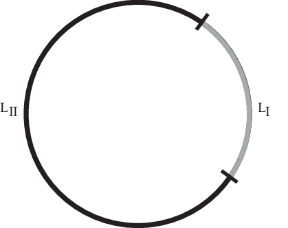
This model was introduced in 1990 [1]; cf. also the related paper [2]. The Casimir energy was calculated for various length ratios of the pieces.

From a physical point of view, there is a well- founded hope that this simple model can give insight in the properties of the vacuum state in two-dimensional quantum field theories in general. The issue of main interest for us here is, however, not to discuss possible practical applications of the model but rather to emphasize the great adaptivity the model has with respect to various regularization methods. The system is remarkably easy to regularize - this circumstance, in fact, supporting the expectation that the model may carry more physical information than has hitherto been recognized. In the paper [1] already mentioned, we made use of a cutoff regularization method whereby a function $f=\exp(-\alpha\omega)$ with $\alpha$ a small positive parameter was introduced. A second regularization method is to make use of complex contour integrations. To our knowledge this method was first applied to the composite string model by Brevik and Elizalde [3]. A separate chapter is devoted to this model in Elizalde’s book on zeta functions [4]. One great advantage of this method is that the multiplicities of the zeros of the dispersion function are automatically taken care of. Third, one may regularize the system by using zeta function methods - as we know, Stuart Dowker has made significant contributions to zeta function theory and related topics in mathematical physics. For the specific piecewise uniform string, it is the Hurwitz kind of zeta function that comes into play.

Instead of assuming only two pieces in the composite string, one can imagine that the string is composed of $2N$ pieces, all of the same length, such that the type I materials and the type II materials are alternating. Maintaining the same relativistic property as before, one will find that also this kind of system is easily regularizable and tractable analytically in general. There are by now several papers devoted to the study of the composite string in its various facets; cf. Refs. [5, 6, 7, 8, 9, 10, 11, 13, 14]. As for possible physical applications of the model, we may also mention the paper of Lu and Huang [15], discussing the Casimir energy for a composite Green-Schwarz superstring.

It ought to be stressed again that the regularizability of the string model relies upon the relativistic condition (1). If this condition were abandoned, the formalism would at once be ambiguous and its predictions obscure. An interesting point in this context is to note the close relationship with the electromagnetic theory in a dielectric medium when the product of the permittivity and the permeability is equal to one (sometimes called an isorefractive medium). While Casimir theories for isorefractive media are easily tractable, the corresponding theory for an ordinary (non-isorefractive) medium would be difficult to construct. For recent papers along these lines, the reader may consult Refs. [16, 17].

There have been further developments of the composite string theory in recent years. We may mention the extension to the so-called quantum spring model [18], where a helix boundary condition for a scalar massless field is imposed. The Casimir forces in the longitudinal and transverse directions for the spring are calculated, using zeta regularization, and the analogue to Hooke’s law in elasticity is recovered when the pitch of the spring is small. Higher dimensions are also envisaged [19]. The fermionic Casimir effect with helix boundary condition is considered in Ref. [20], and the scalar field with a helix torus boundary condition in higher dimension is considered in Ref. [21].

As a proposal for future work, we mention that there may be a connection between the phases of the piecewise uniform (super) string and the Bekenstein-Hawking entropy associated with this string. The entropy, as known, can be derived by counting black hole microstates, and it is natural to expect that the deviation from spatial homogeneity present in the composite string model could influence that sort of calculations.

We ought here to mention the interesting analogy that seems to exist between the composite string model and the so-called quantum star graph model. Fulling et al. [22] recently studied vacuum energy and Casimir forces in one-dimensional quantum graphs (pistons), and found that the piston force could be attractive or repulsive depending on the number of edges. It may be that the mathematical similarities between these two kinds of theories reflect a deeper physical similarity also. This remains to be explored. Another more recent paper of Harrison and Kirsten [23] studies the zeta functions of quantum graphs.

As mentioned above, the main part of this paper is an updated review of the main properties of the composite string model, at zero, and also at finite, temperature, making use of the different contour regularization methods. The convenience of the recursion formula in the $2N$-case, in particular, as treated in Sec. 6, is in our opinion worth attention. The quantum theory of the two-piece string for the simplifying limiting case of very small tension ratio $x$ between the two pieces is highlighted, and the Hagedorn temperature is given for this kind of model.

As a novel development, we give in Sect. 7 a scalar QFT for a real field $\phi$ residing in a potential $V(z)$ consisting of two linear pieces. The first piece, extending from $z=0$ to $z=1$ has a positive slope, while the second piece $z>1$ forms a horizontal plateau. The main idea behind this kind of potential comes from the two-piece string energy in the limiting case of extreme string tension, the string length ratio being replaced formally by a nondimensional length. The expression for the potential has to be simplified, however, in order to give real solutions for the field. We present the Green function for the problem, and give the expression for the field energy density as a function of $z$ for $z>1$.

The simplest way to regularize the system is to introduce a convergence factor $f=e^{-\alpha\omega_{n}},\quad\alpha\ll 1$ [1], and to multiply the nonregularized expression for $E$ with $f$ before summing over the modes.

We first consider a uniform string, $(x=1)$, which implies

$$\omega_{n}=2\pi n/L,\quad n=1,2,3,...$$

(12)

Since these modes are degenerate, we find for the zero-point energy

$$E_{\rm uniform}=\frac{L}{2\pi\alpha^{2}}-\frac{\pi}{6L}+O(\alpha^{2}).$$

(13)

The limiting case $x\rightarrow 0$ ($T_{II}$ assumed finite) leads to two sequences of modes,

$$\omega_{n}=\pi n/L_{I},\quad\omega_{n}=\pi n/L_{II},\quad n=1,2,3,...$$

(14)

We then obtain

$$E=-\frac{\pi}{24L}\left(s+\frac{1}{s}-2\right).$$

(15)

If $s$ is an odd integer, the dispersion equation yields one degenerate branch, given by

$$\omega L_{I}=\pi n,$$

(16)

and $\frac{1}{2}(s-1)$ nondegenerate branches given by

$$\omega L_{I}=\left\{\begin{array}[]{ll}\pi(n+\beta),\\ \pi(n+1-\beta),\end{array}\right.$$

with $n=1,2,3,...,~0<\beta\leq 1/2$.

When $\alpha\rightarrow 0$:

$$E=\frac{\pi s(s-1)}{12L}-\frac{\pi(s+1)}{4L}\sum_{i=1}^{(s-1)/2}[\beta_{i}^{2}+(1-\beta_{i})^{2}];$$

(17)

the cutoff term drops out.

If $s$ is even, we obtain analogously

$$E=\frac{\pi s(2s+1)}{6L}-\frac{\pi(s+1)}{8L}\sum_{i=1}^{s}[\beta_{i}^{2}+(2-\beta_{i})^{2}],$$

(18)

where each $\beta_{i}$ lies in the interval $0<\beta_{i}\leq 1$.

This powerful method, in the context of Casimir calculations, dates back to van Kampen et al. [24]. As mentioned, the method was first applied to the composite string system in Ref. [3]. The starting point is the argument principle,

$$\frac{1}{2\pi i}\oint\omega\frac{d}{d\omega}\ln g(\omega)d\omega=\sum\omega_{0}-\sum\omega_{\infty},$$

(19)

satisfied for any meromorphic function $g(\omega)$, $\omega_{0}$ being the zeros and $\omega_{\infty}$ the poles of $g(\omega)$ inside the integration contour. The contour is taken to a semicircle of large radius $R$ in the right half $\omega$ plane, closed by a straight line from $\omega=iR$ to $\omega=-iR$. An advance of the method, as mentioned, is that the multiplicities are taken care of automatically.

It is convenient to choose

$$g(\omega)=\frac{F(x)\sin^{2}[(s+1)\omega L_{I}/2]+\sin(\omega L_{I})\sin(s\omega L_{I})}{F(x)+1},\quad{\rm with}~s\geq 1.$$

(20)

This choice allows us to perform partial integrations in the energy integral without encountering any divergences in the boundary terms when $R\rightarrow\infty$. The final result, with $\omega=i\xi$, becomes

$$E=\frac{1}{2\pi}\int_{0}^{\infty}\ln\left|\frac{F(x)+\frac{\sinh(\xi L_{I})\sinh(s\xi L_{I})}{\sinh^{2}[(s+1)\xi L_{I}/2]}}{F(x)+1}\right|d\xi,$$

(21)

This expression holds for all values of $s$, not necessarily integers. As the substitution $s\rightarrow 1/s$ leaves the expression invariant, we may restrict ourselves to the interval $s\geq 1$. If the tension ratio $x\rightarrow 0$, we recover the expression (15).

At finite temperature $T$, where $\xi_{n}=2\pi nT$ with $n=0,1,2,3,...$, we get the corresponding expression $(k_{B}=1)$

$$E(T)=T{\sum_{n=0}^{\infty}}^{\prime}\ln\Big|\frac{F(x)+\frac{\sinh(\xi_{n}L_{I})\sinh(s\xi_{n}L_{I})}{\sinh^{2}[(s+1)\xi_{n}L_{I}/2]}}{F(x)+1}\Big|,$$

(22)

where the prime means that the mode $n=0$ is counted with half weight.

We may define two characteristic frequencies in the problem: (i) the thermal frequency $\omega_{T}=T=\xi_{1}/(2\pi)$, and (ii) the geometric frequency $\omega_{\rm geom}=2\pi/L_{I}$. The case of high temperatures corresponds to $\omega_{T}/\omega_{\rm geom}\geq 1$, when we can approximate

$$E(T)=\frac{1}{2}T\ln\Big|\frac{F(x)+4s/(s+1)^{2}}{F(x)+1}\Big|.$$

(23)

Thus if ”our” universe (I) is small and the ”mirror” universe (II) large ($s\rightarrow\infty$), we have

$$E(T)=-\frac{1}{2}T\ln\left|1+F(x)^{-1}\right|.$$

(24)

In the case of low temperatures, $\omega_{T}/\omega_{\rm geom}\ll 1$, a large number of Matsubara frequencies $\xi_{n}$ is necessary.

General treatises on this elegant regularization method can be found in Refs. [4] and [25]. The first application to the composite string was made by Li et al. [2]. The zeta function of most use in this case is not the Riemann function $\zeta(s)$ but instead the Hurwitz function $\zeta_{H}(s,a)$, originally defined as

$$\zeta_{H}(s,a)=\sum_{n=0}^{\infty}(n+a)^{-s},\quad 0<a<1,\quad\Re s>1.$$

(25)

For practical purposes one needs the property

$$\zeta_{H}(-1,a)=-\frac{1}{2}(a^{2}-a+\frac{1}{6})$$

(26)

of the analytically continued function. The Hurwitz function in the form (25) is defined for $\Re s>1$; it is a meromorphic function with a simple pole in $s=1$. If $\Re s$ is different from unity, the Hurwitz function can be analytically continued to the whole complex plane. In our case, Eq. (26) gives the finite value of the Hurwitz function at $s=-1$.

When using the zeta-function method one has to determine the eigenvalue spectrum explicitly. This is the same property as one encounters when using the cutoff method.

Consider first the uniform string: in this case the Riemann function $\zeta(s)$ is sufficient, giving the zero-point energy

$$E_{\rm uniform}=\frac{2\pi}{L}\zeta_{R}(-1)=-\frac{\pi}{6L},$$

(27)

in agreement with the finite part of Eq. (13). Consider next the composite string, assuming $s$ to be an odd integer. Inserting the degenerate branch eigenvalue spectrum (16) we get

$$E_{\rm degenerate~branch}=-\frac{\pi}{12L_{I}}.$$

(28)

Using the corresponding forms for the double branches we obtain analogously

$$E_{\rm double~branch}=\frac{\pi}{2L_{I}}[\zeta_{H}(-1,\beta)+\zeta_{H}(-1,1-\beta)]$$

$$=\frac{\pi}{6L_{I}}-\frac{\pi}{4L_{I}}[\beta^{2}+(1-\beta)^{2}].$$

(29)

Summing (29) over the $\frac{1}{2}(s-1)$ double branches, and adding (28), we obtain for the composite string’s zero-point energy

$$E_{I+II}=\frac{\pi(s-2)}{12L_{I}}-\frac{\pi}{4L_{I}}\sum_{i=1}^{(s-1)/2}[\beta_{i}^{2}+(1-\beta_{i})^{2}].$$

(30)

Now subtracting off the expression (27) we get

$$E=E_{I+II}-E_{\rm uniform}=\frac{\pi s(s-1)}{12L}-\frac{\pi(s+1)}{4L}\sum_{i=1}^{(s-1)/2}[\beta_{i}^{2}+(1-\beta_{i})^{2}],$$

(31)

in agreement with Eq. (17).

The case of even integers $s$ is treated analogously. The zeta-function method is somewhat easier to implement than the cutoff method.

Our aim is now to sketch the essentials of the quantum theory, for the two-piece string. To allow for a correspondence to the superstring, we allow the number of flat spacetime dimensions $D$ to be an arbitrary integer. In accordance with usual practice, we put now $L=L_{I}+L_{II}=\pi$. The theory will be based on two simplifying assumptions:

(i) The string tension ratio $x\rightarrow 0$. The dispersion relation (10) leads in this case to two different branches of solutions, namely the first branch obeying

$$\omega_{n}(s)=(1+s)n,$$

(32)

and the second branch obeying

$$\omega_{n}(s^{-1})=(1+s^{-1})n,$$

(33)

with $n=\pm 1,\pm 2,\pm 3,....$

(ii) The second assumption is that the length ratio $s$ is an integer, $s=1,2,3,...$.

Let now $X^{\mu}(\sigma,\tau)$ with $\mu=0,1,2,..(D-1)$ be the coordinates on the world sheet. For each branch

$$X^{\mu}=x^{\mu}+\frac{p^{\mu}\tau}{\pi\bar{T}(s)}+\theta(L_{I}-\sigma)X_{I}^{\mu}+\theta(\sigma-L_{I})X_{II}^{\mu},$$

(34)

where $\theta(x)$ is the step function, $x^{\mu}$ the center of mass position, and $p^{\mu}$ the total momentum of the string. The mean tension in the actual limit is $\bar{T}(s)={T_{II}s/(1+s)}$ (we assume $T_{II}$ finite). The string’s translational energy is $p^{0}=\pi\bar{T}(s)$. In the following we consider the first branch only.

In region I we make the expansion

$$X_{I}^{\mu}=\frac{i}{2\sqrt{\pi T_{I}}}\sum_{n\neq 0}\frac{1}{n}\left[\alpha_{n}^{\mu}(s)e^{i(1+s)n(\sigma-\tau)}+\tilde{\alpha}_{n}^{\mu}(s)e^{-i(1+s)n(\sigma+\tau)}\right],$$

(35)

where $\alpha_{-n}^{\mu}=(\alpha_{n}^{\mu})^{*},\,\tilde{\alpha}_{-n}^{\mu}=(\tilde{\alpha}_{n}^{\mu})^{*}$. The action can be expressed as

$$S=-\frac{1}{2}\int d\tau d\sigma T(\sigma)\eta^{\alpha\beta}\partial_{\alpha}X^{\mu}\partial_{\beta}X_{\mu},$$

(36)

where $T(\sigma)=T_{I}+(T_{II}-T_{I})\theta(\sigma-L_{I})$. As the conjugate momentum is $P^{\mu}(\sigma)=T(\sigma)\dot{X}^{\mu},$ we obtain the Hamiltonian

$$H=\int_{0}^{\pi}[P_{\mu}(\sigma)\dot{X}^{\mu}-L]d\sigma=\frac{1}{2}\int_{0}^{\pi}T(\sigma)(\dot{X}^{2}+{X^{\prime}}^{2})d\sigma.$$

(37)

The fundamental condition is that $H=0$ when applied to physical states.

The corresponding expansion of the first branch in region II is

$$X_{II}^{\mu}=\frac{i}{2\sqrt{\pi T_{I}}}\sum_{n\neq 0}\frac{1}{n}\gamma_{n}^{\mu}(s)e^{-i(1+s)n\tau}\cos[(1+s)n\sigma],$$

(38)

with

$$\gamma_{n}^{\mu}(s)=\alpha_{n}^{\mu}(s)+\tilde{\alpha}_{n}^{\mu}(s),\quad n\neq 0.$$

(39)

The condition $x\rightarrow 0$ means that there are only standing waves in region II.

We may now introduce light-cone coordinates $\sigma^{-}=\tau-\sigma,\,\sigma^{+}=\tau+\sigma$. Some calculation shows that the total Hamiltonian can be written as a sum of two parts,

$$H=H_{I}+H_{II},$$

(40)

where

$$H_{I}=\frac{1+s}{4}\sum_{-\infty}^{\infty}[\alpha_{-n}(s)\cdot\alpha_{n}(s)+\tilde{\alpha}_{-n}(s)\cdot\tilde{\alpha}_{n}(s)],$$

(41)

$$H_{II}=\frac{s(1+s)}{8x}\sum_{-\infty}^{\infty}\gamma_{-n}(s)\cdot\gamma_{n}(s).$$

(42)

The mass $M$ of the string determined by $M^{2}=-p^{\mu}p_{\mu}$,

$$M^{2}=\pi T_{II}s\sum_{n=1}^{\infty}\left[\alpha_{-n}(s)\cdot\alpha_{n}(s)+\tilde{\alpha}_{-n}(s)\cdot\tilde{\alpha}_{n}(s)+\frac{s}{2x}\gamma_{-n}(s)\cdot\gamma_{n}(s)\right].$$

(43)

Recall that this is the contribution from first branch only. The expression is valid for even/odd values of $s$.

Consider now the quantization of the first branch modes. We impose the conditions

$$T_{I}[\dot{X}^{\mu}(\sigma,\tau),X^{\nu}(\sigma^{\prime},\tau)]=-i\delta(\sigma-\sigma^{\prime})\eta^{\mu\nu}$$

(44)

in region I, and

$$T_{II}[\dot{X}^{\mu}(\sigma,\tau),X^{\nu}(\sigma^{\prime},\tau)]=-i\delta(\sigma-\sigma^{\prime})\eta^{\mu\nu}$$

(45)

in region II (the other commutators vanish). Then introducing creation and annihilation operators via

$$\alpha_{n}^{\mu}(s)=\sqrt{n}a_{n}^{\mu}(s),\quad\alpha_{-n}^{\mu}(s)=\sqrt{n}{a_{n}^{\mu}}^{\dagger}(s),$$

(46)

$$\gamma_{n}^{\mu}(s)=\sqrt{4nx}c_{n}^{\mu}(s),\quad\gamma_{-n}(s)=\sqrt{4nx}{c_{n}^{\mu}}^{\dagger}(s),$$

(47)

one arrives at the conventional commutation relations

$$[a_{n}^{\mu}(s),{a_{m}^{\nu}}^{\dagger}(s)]=\delta_{nm}\eta^{\mu\nu},\quad[c_{n}^{\mu}(s),{c_{m}^{\nu}}^{\dagger}(s)]=\delta_{nm}\eta^{\mu\nu},$$

(48)

for $n,m\geq 1$.

Now introduce $t(s)$ as

$$t(s)=\pi\bar{T}(s)=\frac{\pi s}{1+s}T_{II},$$

(49)

and put $D=26$, the usual dimension for the bosonic string. The condition $H=H_{I}+H_{II}=0$ leads to

$$M^{2}=t(s)\sum_{i=1}^{24}\sum_{n=1}^{\infty}\omega_{n}(s)[{a_{ni}}^{\dagger}(s)a_{ni}(s)+{\tilde{a}_{ni}}^{\dagger}(s)\tilde{a}_{ni}(s)-2]$$

$$+2st(s)\sum_{i=1}^{24}\sum_{n=1}^{\infty}\omega_{n}(s)[{c_{ni}}^{\dagger}(s)c_{ni}(s)-1],$$

(50)

and the free energy becomes

$$F=-\frac{1}{24}(s+\frac{1}{s}-2)-2^{-40}\pi^{-26}t(s)^{-13}\int_{0}^{\infty}\frac{d\tau_{2}}{\tau_{2}^{14}}\int_{-1/2}^{1/2}d\tau_{1}$$

$$\times\left[\theta_{3}\left(0\Big|\frac{i\beta^{2}t(s)}{8\pi^{2}\tau_{2}}\right)-1\right]\Big|\eta[(1+s)\tau]\Big|^{-48}\eta[s(1+s)(\tau-\bar{\tau})]^{-24}$$

(51)

Here $\tau=\tau_{1}+i\tau_{2}$ is the $\rm Teichm\ddot{u}ller$ parameter,

$$\eta(\tau)=e^{\pi i\tau/12}\prod_{n=1}^{\infty}\left(1-e^{2\pi in\tau}\right)$$

(52)

is the Dedekind $\eta$-function, and

$$\theta_{3}(v|x)=\sum_{n=-\infty}^{\infty}e^{ixn^{2}+2\pi ivn}$$

(53)

is the Jacobi $\theta_{3}$ - function. From this the thermodynamic quantities such as internal energy $U$ and entropy $S$ can be calculated,

$$U=\frac{\partial(\beta F)}{\partial\beta},\quad S=\beta^{2}\frac{\partial F}{\partial\beta}.$$

(54)

Finally, let us consider the limiting case in which one of the string pieces is much shorter than the other. Physically this case is of interest, since it corresponds to a point mass sitting on a string. Since we have assumed that $s\geq 1$, this case corresponds to $s\rightarrow\infty$. We let the tension $T_{II}$ be fixed, though arbitrary. It is seen that the critical temperature goes to infinity so that the free energy $F$ is always ultraviolet finite. In this limit we obtain [10]

$$F_{(\beta\rightarrow 0)}=-\frac{s}{24}-(8\pi^{3}T_{II})^{-13}\int_{0}^{\infty}\frac{d\tau_{2}}{\tau_{2}^{14}}\int_{-1/2}^{1/2}d\tau_{1}$$

$$\times\exp\left(-\frac{\beta^{2}T_{II}}{8\pi\tau_{2}}\right)|\eta[(1+s)\tau]|^{-48}\,\eta[s(1+s)(\tau-\bar{\tau})]^{-24}.$$

(55)

The second term goes to zero for large $s$. Physically speaking, the linear dependence of the first term reflects that the Casimir energy of a little piece of string embedded in an essentially infinite string is for dimensional reasons inversely proportional to the length $L_{I}$. Thus

$$F\propto 1/L_{I}=(1+s)/\pi\approx s/\pi.$$

(56)

In the same way one can consider the Casimir theory for a string of length $L$ divided into three pieces, all of the same length. The theory for this case was given in Refs. [6] and [9]. Here, we shall consider instead a string divided into $2N$ pieces of equal length, of alternating type I (type II) material. The string is relativistic, i.e. it satisfies the condition (1), as above. The basic formalism for arbitrary integers $N$ was established in Ref. [5], but the Casimir energy was there calculated in full only for the case $N=2$. A full calculation was given in Ref. [8], cf. also Ref. [9]. A key point in Ref. [8] was the derivation of a new recursion formula, applicable for general integers $N$.

Now define the symbols $p_{N}$ and $\alpha$,

$$p_{N}=\frac{\omega L}{N},\quad\alpha=\frac{1-x}{1+x},$$

(57)

and recall that $x=T_{I}/T_{II}$. The eigenfrequencies are determined from

$$\rm{Det}\left[{\bf M}_{2N}(x,p_{N})-{\bf 1}\right]=0,$$

(58)

where

$${\bf M}_{2N}(x,p_{N})=\left[\frac{(1+x)^{2}}{4x}\right]^{N}{\bf\Lambda}^{N}(\alpha,p_{N}),$$

$${\bf\Lambda}(\alpha,p)=\left(\begin{array}[]{ll}a&b\\ b^{*}&a^{*}\end{array}\right),$$

(59)

and

$$a=e^{-ip}-\alpha^{2},\quad b=\alpha(e^{-ip}-1).$$

The expression (59) relies upon a compact recursion formula which serves to simplify the calculation (more details are given in Ref. [8]). One can now calculate the eigenvalues of $\bf\Lambda$, and express the elements of ${\bf M}_{2N}$ as powers of these.

The Casimir energy can now be found. By means of contour integration we can write, for arbitray $x$ and arbitray integers $N$, at zero temperature,

$$E_{N}(x)=\frac{N}{2\pi L}\int_{0}^{\infty}\ln\left|\frac{2(1-\alpha^{2})^{N}-[\lambda_{+}^{N}(iq)+\lambda_{-}^{N}(iq)]}{4\sinh^{2}(Nq/2)}\right|dq,$$

(60)

where $\lambda_{\pm}$ are eigenvalues of $\bf\Lambda$, for imaginary arguments $iq$, of the dispersion equation. Explicitly,

$$\lambda_{\pm}(iq)=\cosh q-\alpha^{2}\pm[(\cosh q-\alpha^{2})^{2}-(1-\alpha^{2})^{2}]^{1/2}.$$

(61)

Evaluation of the integral shows that $E_{N}(x)<0,~|E_{N}(x)|$ increasing with increasing $N$. A string is thus in principle able to diminish its zero-point energy by dividing itself into a larger number of pieces of alternating type I (or II) material. If this property has physical significance, is at present unknown.

If $x\rightarrow 0$ the integral can be solved exactly,

$$E_{N}(0)=-\frac{\pi}{6L}(N^{2}-1).$$

(62)

The generalization of the expression (60) to the case of finite temperatures is easily achieved following the same procedure as above.

As an alternative method one can instead of contour integration make use of the zeta-function method. One then has to determine the spectrum explicitly and thereafter put in the degeneracies by hand. The latter method is therefore most suitable for low $N$.

Scaling invariance

A rather unexpected scaling invariance property of the Casimir energy becomes apparent if we examine the behavior of the function $f_{N}(x)$ defined by

$$f_{N}(x)=\frac{E_{N}(x)}{E_{N}(0)},\quad 0<f_{N}(x)<1.$$

(63)

This function lies between zero and one. By calculating $E_{N}(x)$ (usually numerically) as a function of $x$ for a fixed value of $N$, we find that the resulting curve for $f_{N}(x)$ is practically the same, irrespective of the value of $N$, as long as $N\geq 2$. (The case $N=1$ is exceptional, since $E_{1}(x)=0$.) Numerical trials show that the analytic form

$$f_{N}(x)\rightarrow f(x)=(1-\sqrt{x})^{5/2}$$

(64)

is a useful approximation, especially in the interval $0<x<0.45$ [11].

At finite temperature the expression for the Casimir energy becomes

$$E_{N}^{T}(x)=T{\sum_{n=0}^{\infty}}^{\prime}\ln\left|\frac{2(1-\alpha^{2})^{N}-[\lambda_{+}^{N}(i\xi_{n}L/N)+\lambda_{-}^{N}(i\xi_{n}L/N)]}{4\sinh^{2}(\xi_{n}L/2)}\right|,$$

(65)

where $\lambda_{\pm}(i\xi_{n}L/N)$ are given by Eq. (61) with $q\rightarrow q_{n}=\xi_{n}L/N$. It is here useful to note that

$$\lambda_{+}(iq_{n})+\lambda_{-}(iq_{n})=2(\cosh q_{n}-\alpha^{2}).$$

(66)

There are several special cases of interest. First, if the string is uniform ($x=1$), we get $E_{N}^{T}(1)=0$. This is as expected, as the Casimir energy is a measure of the string’s inhomogeneity. If $N=1$, $x$ arbitrary, we also get a vanishing result, $E_{1}^{T}(x)=0$. In particular, if $x\rightarrow 0$ we get the simple formula

$$E_{N}(0)=2T{\sum_{n=0}^{\infty}}^{\prime}\ln\left|\frac{2^{N}\sinh^{N}(\xi_{n}L/2N)}{2\sinh(\xi_{n}L/2)}\right|.$$

(67)

,

Consider the following problem in the quantum theory of a massless scalar field $\phi(x)$ ($x={\bf r},t$) in three-dimensional space if there is a potential $V=V(z)$ varying in the $z$ direction only,

$$V(z)=-\left(z+\frac{1}{z}-2\right),\quad 0\leq z<\infty.$$

(68)

One may ask: is it possible to calculate the field energy density $u(z)$ analytically as a function of $z$ for such a case? We see that the potential $V$ reflects actually our previous expression (15) for the Casimir energy $E$ of a two-piece string, in the limit when the string tension ratio $x=T_{I}/T_{II}$ goes to zero, if the length ratio $s=L_{II}/L_{I}$ is replaced with the ”length” $z$. The ansatz (68) is given in a nondimensional form, for simplicity. The zero value of $V$ at $z=1$ corresponds to the previous zero Casimir energy $E$ at $s=1$.

Evidently, the relationship with our Casimir theory is quite formal. Nevertheless, we find it of interest to explore the QFT problem based upon Eq. (68) in its own right , so also because of the recent interest in this kind of scalar field models in the recent literature.

Let us first look at some consequences of using the potential (68) as it stands. The field equation

$$\left(\Box+z+\frac{1}{z}-2\right)\phi(x)=0,$$

(69)

when combined with the Fourier transform

$$\phi(x)=\int\frac{d\omega}{2\pi}\frac{d\bf k}{(2\pi)^{2}}e^{-i\omega t+i{\bf k\cdot r}}\phi(z),$$

(70)

leads to the following equation

$$\phi^{\prime\prime}(z)+\left(z+\frac{1}{z}-\kappa^{2}-2\right)\phi(z)=0.$$

(71)

Here $\bf k$ means the wave vector in the $xy$ plane, transverse to the $z$ axis, and $\kappa^{2}$ is defined as

$$\kappa^{2}={\bf k}^{2}-\omega^{2}.$$

(72)

We have looked for exact solutions of Eq. (71) using Mathematica, without finding an exact solution. It is of interest nevertheless to consider some limiting cases. First, if $z\rightarrow 0$ the field equation reduces to

$$\phi^{\prime\prime}(z)+\frac{1}{z}\phi(z)=0,$$

(73)

admitting the solution

$$\phi(z)\propto\sqrt{z}J_{1}(2\sqrt{z}),$$

(74)

(infinities at the origin discarded). Here $J_{1}$ is the Bessel function of the first kind. Next, in the region where $z$ lies around unity we get

$$\phi^{\prime\prime}(z)-\kappa^{2}\phi(z)=0,$$

(75)

implying that $\phi$ contains linear combinations of $e^{\kappa z}$ and $e^{-\kappa z}$. Finally, as $z\rightarrow\infty$ the reduced equation takes the form

$$\phi^{\prime\prime}(z)+z\phi(z)=0,$$

(76)

which has complex solutions, $Ai[(-1)^{1/3}z]$ and $Bi[(-1)^{1/3}z]$, $Ai$ and $Bi$ being the Airy functions. The complex nature of these solutions are related to the negative slope of the potential $V$ when $z>1$. In our case such solutions are not of interest; we are looking for real solutions for $\phi(z)$.

We thus conclude that in order to construct a meaningful QFT for the real field, we have to replace the expression for $V$ above with a simpler form. Our choice in the following will be the most simple and natural one, namely to choose a linear wall, increasing from $z=0$ with a positive constant slope to a maximum value of $V=0$ at $z=1$. For higher $z$ we assume there to be a constant plateau. Thus, our potential assumed in the following will have the form

$$V(z)=z-1,\quad 0\leq z<1,$$

$$V(z)=0,\quad z>1.$$

(77)

In the first equation the slope is chosen equal to unity for simplifying reasons. Our choice (77) is of essentially the same form as that considered recently by Milton [28]; cf. also related papers by Bouas et al. [29].

The Green function $G(x,x^{\prime})$ with $V(z)$ given by Eq. (77) satisfies the governing equation

$$\left(\frac{\partial^{2}}{\partial t^{2}}-\nabla^{2}+V(z)\right)G(x,x^{\prime})=\delta(x-x^{\prime}).$$

(78)

With the Fourier transform

$$G(x,x^{\prime})=\int\frac{d\omega}{2\pi}\frac{d\bf k}{(2\pi)^{2}}e^{-i\omega(t-t^{\prime})+i\bf k\cdot(r-r^{\prime})}g(z,z^{\prime}),$$

(79)

we get the following equation for the Fourier component

$$\left(\frac{\partial^{2}}{\partial z^{2}}-\kappa^{2}-V(z)\right)g(z,z^{\prime})=-\delta(z-z^{\prime}).$$

(80)

We perform a complex frequency rotation $\omega\rightarrow i\zeta$, so that $\kappa^{2}\rightarrow{\bf k}^{2}+\zeta^{2}$.

Assume in the following that $z^{\prime}$ lies on the horizontal plateau, $z^{\prime}>1$. Then,

$$0\leq z<1:\quad g(z,z^{\prime})=A(z^{\prime}){\rm Ai}(\kappa^{2}-1+z)+B(z^{\prime}){\rm Bi}(\kappa^{2}-1+z),$$

$$\noindent z>1:\quad g(z,z^{\prime})=\frac{1}{2\kappa}e^{-\kappa|z-z^{\prime}|}+C(z^{\prime})e^{-\kappa(z-1)},$$

(81)

where we have adopted the boundary condition $G\rightarrow 0$ at $z\rightarrow\infty$. At $z=0$ we impose the Dirichlet condition:

$$A(z^{\prime}){\rm Ai}(\kappa^{2}-1)+B(z^{\prime}){\rm Bi}(\kappa^{2}-1)=0.$$

(82)

To determine the functions $A,B$ and $C$ we need two more boundary conditions, namely that $G$ itself as well as its derivative are continuous at $z=1$:

$$A(z^{\prime}){\rm Ai}(\kappa^{2})+B(z^{\prime}){\rm Bi}(\kappa^{2})=\frac{1}{2\kappa}e^{-\kappa z^{\prime}}+C(z^{\prime}),$$

$$A(z^{\prime}){\rm Ai}^{\prime}(\kappa^{2})+B(z^{\prime}){\rm Bi}^{\prime}(\kappa^{2})=\frac{1}{2}e^{-\kappa z^{\prime}}-\kappa C(z^{\prime}).$$

(83)

The solution to this set of equations can be written as

$$A(z^{\prime})=\frac{{\rm Bi}(\kappa^{2}-1)}{{\rm Ai}(\kappa^{2}){\rm Bi}(\kappa^{2}-1)-{\rm Ai}(\kappa^{2}-1){\rm Bi}(\kappa^{2})}\,\frac{e^{-\kappa z^{\prime}}}{Q},$$

$$B(z^{\prime})=-\frac{{\rm Ai}(\kappa^{2}-1)}{{\rm Ai}(\kappa^{2}){\rm Bi}(\kappa^{2}-1)-{\rm Ai}(\kappa^{2}-1){\rm Bi}(\kappa^{2})}\,\frac{e^{-\kappa z^{\prime}}}{Q},$$

$$C(z^{\prime})=-\left(\frac{1}{2}-\frac{1}{Q}\right)e^{-\kappa z^{\prime}},$$

(84)

where we have defined $Q$ as

$$Q=\kappa+\frac{{\rm Ai}^{\prime}(\kappa^{2}){\rm Bi}(\kappa^{2}-1)-{\rm Ai}(\kappa^{2}-1){\rm Bi}^{\prime}(\kappa^{2})}{{\rm Ai}(\kappa^{2}){\rm Bi}(\kappa^{2}-1)-{\rm Ai}(\kappa^{2}-1){\rm Bi}(\kappa^{2})}.$$

(85)

These expressions are complicated. It is of interest to consider approximate values in limiting cases. Let us assume the case of high frequencies, implying that $\kappa^{2}={\bf k}^{2}+\zeta^{2}\gg 1$. Then, we have as rough approximations [30]

$${\rm Ai}(x)\sim\frac{e^{-\xi}}{2\sqrt{\pi}x^{1/4}},\quad{\rm Bi}(x)\sim\frac{e^{\xi}}{\sqrt{\pi}x^{1/4}},$$

(86)

where $\xi=\frac{2}{3}x^{3/2}$. Together with the Wronskian for general argument, $W\{{\rm Ai}(x),{\rm Bi}(x)\}=\frac{1}{\pi}$, this yields

$$A(z^{\prime})\sim-\sqrt{\frac{\pi}{\kappa}}\,e^{-\kappa(z^{\prime}+1)}\exp\left[\frac{2}{3}(\kappa^{2}-1)^{3/2}\right],$$

$$B(z^{\prime})\sim\frac{1}{2}\sqrt{\frac{\pi}{\kappa}}\,e^{-\kappa(z^{\prime}+1)}\exp\left[-\frac{2}{3}(\kappa^{2}-1)^{3/2}\right],$$

$$Q\rightarrow 2\kappa\quad(C(z^{\prime})\rightarrow 0).$$

(87)

References

- [1] Brevik, I. and Nielsen, H. B. 1990 Phys. Rev. D 41, 1185.
- [2] Li, X., Shi, X. and Zhang, J. 1991 Phys. Rev. D 44, 560.
- [3] Brevik, I. and Elizalde, E. 1994 Phys. Rev. D 49, 5319.
- [4] Elizalde, E. 1995 Ten Physical Applications of Spectral Zeta Functions (Berlin-Springer), Chapter 7.
- [5] Brevik, I. and Nielsen, H. B. 1995 Phys. Rev. D 51, 1869.
- [6] Brevik, I., Nielsen, H. B. and Odintsov, S. D. 1996 Phys. Rev. D 53, 3224.
- [7] Bayin, S. S., Krisch, J. P. and Ozcan, M. 1996 J. Math. Phys. 37, 3662.
- [8] Brevik, I. and Sollie, R. 1997 J. Math. Phys. 38, 2774.
- [9] Berntsen, M. H., Brevik, I. and Odintsov, S. D. 1997 Ann. Phys. NY 257, 84.
- [10] Brevik, I., Bytsenko, A. A. and Nielsen, H. B. 1998 Class. Quant. Grav. 15, 3383.
- [11] Brevik, I., Elizalde, E., Sollie, R. and Aarseth, J. B. 1999 J. Math. Phys. 40, 1127.
- [12] Hadasz, L., Lambiase, G. and Nesterenko, V. V. 2000 Phys. Rev. D 62, 025011.
- [13] Brevik, I., Bytsenko, A. A. and Pimentel, B. M. 2003 In: Theoretical Physics 2002, Part 2, p. 117. Eds.: T. F. George and H. F. Arnoldus (New York: Nova Sci. Publ.).
- [14] Brevik. I. 2011 In: Cosmology, Quantum Vacuum and Zeta Functions. In honor of Prof. Emilio Elizalde, Springer Proceedings in Physics 127, Eds. S. D. Odintsov, D. Saez-Gomez and S. Xambo-Descamps, p. 57 [arXiv:1007.1354].
- [15] Lu, J. and Huang, B. 1998 Phys. Rev. D 57, 5280.
- [16] Brevik, I., Ellingsen, S. Å and Milton, K. A. 2009 Phys. Rev. E 79, 041120.
- [17] Ellingsen, S. Å., Brevik, I. and Milton, K. A. 2009 Phys. Rev. E 80, 021125.
- [18] Feng, C. J. and Li, X. Z. 2010 Phys. Lett. B 691, 167.
- [19] Zhai, X. H., Li, X. Z. and Feng, C. J. 2011 Mod. Phys. Lett. A 26, 669.
- [20] Zhai, X. H., Li, X. Z. and Feng, C. J. 2011 Eur. Phys. J. C 71, 1654.
- [21] Zhai, X. H., Li, X. Z. and Feng, C. J. 2011 arXiv:1107.4846 [hep-th].
- [22] Fulling, S. A., Kaplan, L. and Wilson, J. H. 2007 Phys. Rev. A 76, 012118.
- [23] Harrison, J. M. and Kirsten, K. 2011 J. Phys. A: Math. Theor. 44, 235301.
- [24] van Kampen, N. G., Nijboer, B. R. A. and Schram, K. 1968 Phys. Lett. A 26, 307.
- [25] Elizalde, E., Odintsov, S. D., Romeo, A., Bytsenko, A. A. and Zerbini, S. 1994 Zeta Regularization Techniques with Applications (Singapore: World Scientific).
- [26] Brevik, I., Bytsenko, A. A. and Goncalves, A. E. 1999 Phys. Lett. B 453, 217.
- [27] Hagedorn, R, 1965 Suppl. Il Nuovo Cimento 3, 147.
- [28] K. A. Milton, Phys. Rev. D 84, 065028 (2011),
- [29] J. D. Bouas, S. A. Fulling, F. D. Mera, K. Thapa, C. S. Trendafilova and J. Wagner, arXiv:1106.1162 [Proc. Symp. Pure Math., to be published].
- [30] NIST Handbook of Mathematical Functions, edited by Frank W. J. Olver et al. (Cambridge University Press, 2010), Eqs.9.7.15 and 9.7.16.
- [31] Meinardus, G. 1954 Math. Z. 59, 338; 61, 289.