Global Constraints on Effective Dark Matter Interactions:
Relic Density, Direct Detection, Indirect Detection, and Collider
Abstract
An effective interaction approach is used to describe the interactions between the spin 0 or spin 1/2 dark matter particle and the degrees of freedom of the standard model. This approach is applicable to those models in which the dark matter particles do not experience the standard-model interactions, e.g., hidden-sector models. We explore the effects of these effective interaction operators on (i) dark matter relic density, (ii) spin-independent and spin-dependent dark matter-nucleon scattering cross sections, (iii) cosmic antiproton and gamma ray fluxes from the galactic halo due to dark matter annihilation, and (iv) monojet and monophoton production plus missing energy at the Tevatron and the Large Hadron Collider (LHC). We combine the experimental data of relic density from WMAP7, spin-independent cross section from XENON100, spin-dependent cross section from XENON10, ZEPLIN-III, and SIMPLE, cosmic antiproton flux from PAMELA, cosmic gamma-ray flux from -LAT, and the monojet and monophoton data from the Tevatron and the LHC, to put the most comprehensive limits on each effective operator.
I Introduction
The presence of cold dark matter (CDM) in our Universe is now well established by a number of observational experiments, especially the very precise measurement of the cosmic microwave background radiation in the Wilkinson Microwave Anisotropy Probe (WMAP) experiment [1]. The measured value of the CDM relic density is
| (1) |
where is the Hubble constant in units of km/Mpc/s. Though the gravitation nature of the dark matter (DM) is commonly believed to be well established, its particle nature remains alluring except that it is nonbaryonic and to a high extent electrically neutral.
One of the most appealing and natural CDM particle candidates is the weakly-interacting massive particle (WIMP). If the dark matter, generically denoted by here, is thermally produced in the early Universe, the required annihilation cross section is right at the order of weak interaction. There may be a dynamical connection between the dark matter and weak-scale physics. The relation between the fractional relic density of relative to the critical density and its thermal annihilation cross section can be given by the following simple formula [2]
| (2) |
with being the annihilation cross section of the dark matter around the time of freeze-out, at which the annihilation rate could no longer catch up with the Hubble expansion rate of the Universe. Assuming the measured to be saturated by a single component WIMP, its annihilation cross section should be about pb or . This is exactly the size of the cross section that one expects from a weak interaction process, which implies an appreciable size of production rate of the WIMP at the Large Hadron Collider (LHC) as well as the event rates for direct and indirect searches that reach the sensitivities of dark matter experiments like XENON100 [3] and -LAT [4, 5] respectively.
There have been many proposed candidates for the dark matter. Without committing to any particular DM model so as to perform a model independent analysis, we adopt an effective interaction approach to describe the interactions of the dark matter particle with the standard model (SM) particles. Recently, there have been a number of works in this approach that deals with different observable signals in various experiments [6, 7, 8, 9, 10, 11, 12], [13, 14, 15, 16], [17, 18, 19, 20, 21, 22, 23, 24], [25, 26, 27, 28]. One simple realization of the effective interaction approach is that the dark matter particle exists in a hidden sector, which communicates to the SM sector via a heavy degree of freedom in the connector sector. At energy scale well below this heavy mediator the interactions can be conveniently described by a set of effective interactions. The strength of each interaction depends on the nature of the dark matter particle and the mediator. A few models that can give rise to some of the operators in this analysis are described in the appendix. However, note that some popular dark matter models, such as supersymmetry, cannot be correctly described by this effective-interaction appraoch, because the dark matter particles themselves also experience the SM interactions. In this work, we will consider various spin nature of the dark matter particle including Dirac and Majorana for fermionic dark matter, as well as real and complex scalar. The most important set of interactions among the fermionic dark matter and the light fermions are described by the effective operators , where and are general Dirac matrices contracted with appropriate Lorentz indices. We will discuss these and other operators in more details in the next section.
One of the most anticipated signals of dark matter at hadronic colliders is a large missing energy in association with jets, photons, or leptons, such as monojet and monophoton plus large missing-energy signatures. For example, if we take one of the operators, , and attach a gluon or a photon to a quark leg, it will give rise to a monojet or a monophoton plus missing energy event. The Tevatron experiments and the LHC experiments have been actively searching for these signatures in some other context, such as large extra dimensions [29]. We will use the most updated data on monojet and monophoton production from the LHC [30] and the Tevatron [31, 32, 33] to constrain each effective operator. It turns out that the limits from the LHC and Tevatron are comparable to those obtained from indirect detection data (PAMELA [34, 35] and -LAT [4, 5]), but inferior to those obtained from direct detection data (XENON100 [3] and CDMS [36]) if a particular operator contributes to spin-independent cross sections. Some recent works in this direction have been in Refs. [6, 7, 8, 9, 10, 11, 12, 13, 14, 15, 16, 17, 18, 19, 20, 21, 22, 23, 24, 25, 26, 27, 28].
Dark matter annihilation in the galactic halo gives rise to a number of observable signals, including excess in positron flux, antiproton flux, and gamma-ray over the corresponding cosmic backgrounds. The most current positron flux and antiproton flux data come from PAMELA [34, 35]. The positron-fraction spectrum showed an uprising trend up to about 100 GeV [34]. 11 1 A very recent result from -LAT [4] showed that the uprising trend continues to about 150 GeV. Nevertheless, the antiproton flux is consistent with the expected cosmic background [35]. The effective operators such as can give rise to dark matter annihilation into light quarks, which will eventually hadronize into antiprotons. In Refs. [13, 14, 15, 16] the effects of dark matter annihilation on positron flux and antiproton flux were studied. It was shown that the antiproton flux data can give a better constraint on the effective dark matter interactions than the positron flux data [13]. So in this work we focus on antiproton flux data when we use antimatter search experiments to constrain the effective dark matter interactions.
Another powerful set of indirect detection data comes from the gamma ray due to dark matter annihilation in the galactic halo. The data from the extragalactic sources contain large uncertainties, such that we concentrate on the galactic data in this work. Currently, the best data come from the -LAT experiment [5]. It detects gamma rays in sub-GeV region to hundreds of GeV from all directions , i.e., including Galactic Center (GC) , low-latitude , mid-latitude , and high latitude . The data on the photon spectrum from the low-latitude [5] recorded by the -LAT indicated a continuous spectrum and mostly consistent with the known backgrounds. We can therefore use the data to constrain on additional sources of gamma-ray, namely, the annihilation of the dark matter into quarks, followed by fragmentation into neutral pions, which further decay into photons. Some recent works in using the -LAT to constrain various models or effective dark matter interactions can be found in Refs. [17, 18, 19, 20, 21, 22, 23, 24].
Another important method of detecting DM is through the direct collision between the DM particles in the halo with the nuclei of the detecting materials. The DM particles then lose a fraction of the kinetic energy to the nuclei, which can be detected by a phonon-type or scintillation-type or ionization-type signal or some combinations of these types. Since the energy transfer is only of order keV and the event rate is extremely low, an almost background-free environment is needed. The most recent result comes from the XENON100 Collaboration [3], which did not see any signal events and obtained limits on the spin-independent (SI) cross sections versus the DM mass. The 90% CL upper limit on for GeV. We are going to use the limits presented in Ref. [3] to constrain the effective operators.
In this work, we are going to constrain each operator from the combined data sets on relic density (WMAP), direct detection (XENON, ZEPLIN and SIMPLE), cosmic antiproton flux (PAMELA), cosmic gamma-ray flux (-LAT), and monojet and monophoton production (Tevatron and LHC). The organization of this work is as follows. We describe the set of effective operators for fermionic and scalar DM and describe their nonrelativistic limits in Sec. II. In Sec. III, we calculate the relic density assuming production of DM from the thermal equilibrium and by solving the Boltzmann equation. In Sec. IV, we calculate both the spin-independent (SI) and spin-dependent (SD) cross sections and constrain each operator by the XENON100 [3], XENON10 [37], ZEPLIN [38], and SIMPLE [39] data. In Sec. V and VI, we calculate the cosmic antiproton and gamma-ray flux, respectively, and constrain each operator from the most current data. In Sec. VII, we calculate monojet and monophoton production at the Tevatron and LHC, and use the most current data to constrain each operator. In Sec. VIII, we perform a combined analysis by adding the chi-square of each data set. We conclude in Sec. IX.
Before we close this introduction section we would spell out the improvements that are achieved in this work.
- 1.
The constraint from the LHC monojet and monophoton production was only recently done in Refs. [11, 12]. We perform an independent analysis here. 22 2 There are recent works that consider light mediators between the SM fermions and the dark matter [40], the unitarity bound of the operators [41], and light dark matter [42].
- 2.
We perform a full calculation of the relic density by solving the Boltzmann equation.
- 3.
- 4.
We combine all data sets in the combined analysis. The resulting limits will be the most stringent so far. 33 3 A generalized analysis of WIMP in nonrelativistic limit can be found in Ref. [43].
Based on these improvements and by demanding an operator not to give too much relic density to the Universe and satisfying the current experimental constraints from direct and indirect detection, and from collider data, a vast number of effective DM operators are indeed ruled out. The conclusion obtained here is important for building an effective model for the dark matter.
II Effective Dark Matter Interactions
For simplicity, we will assume there is only one component of dark matter denoted by and it is a standard model singlet. Here the can stand for a Dirac or Majorana fermion, real or complex scalar, depending on the context. Also, stands for a SM fermion, including quarks and leptons. We will include all quarks and leptons in our analysis. We briefly discuss in the Appendix a few hidden-sector models that can give rise to some of the operators used in this work in certain limits. For dark matter of spin 1 and spin 3/2, the reader may refer to the works in Refs. [27, 28].
The first set of operators that we consider is for fermionic DM. Its effective interactions with a pair of fermions include vector-, axial-vector, or tensor-type exchanges, given by the following dimension 6 operators
| (3) | |||||
| (4) | |||||
| (5) | |||||
| (6) | |||||
| (7) | |||||
| (8) |
where is the heavy mass scale for the connector sector that has been integrated out and is an effective coupling constant of order that can be absorbed into . It is understood that for Majorana fermion the vector and tensor structures are absent.
Next set of operators are for fermionic DM associated with (pseudo) scalar-type exchange
| (9) | |||||
| (10) | |||||
| (11) | |||||
| (12) |
The dependence in the coupling strength is included for scalar-type interactions because this factor appears naturally from dark matter models with scalar exchange diagrams. Another light degree of freedom that couples to the fermionic dark matter is the gluon field
| (13) | |||||
| (14) | |||||
| (15) | |||||
| (16) |
For operators involving gluons, the factor of strong coupling constant is also included because these operators are induced at one loop level and evaluated at the scale where is the dark matter mass.
Finally, we also write down the corresponding operators for complex scalar DM.
| (17) | |||||
| (18) | |||||
| (19) | |||||
| (20) | |||||
| (21) | |||||
| (22) |
We note that for real scalar dark matter the vector couplings in Eqs.(17) and (18) are absent. In what follows, we simply focus on the complex scalar dark matter. Note also that we have redefined the coefficients of some of the operators, which are different from our previous works [13, 24], such that they can conform with the normalization for the nucleon matrix elements used in the literature for the direct detection experiments.
In Ref. [13], we showed that in the calculation of the annihilation cross section for the DM relic density, the relative importance of each operator can be understood by considering the nonrelativistic expansion of the operator and studying the velocity dependence. We briefly review this matter here for convenience. In the nonrelativistic limit, the spinors for the Dirac DM and annihilation are and where and are two-components Pauli spinors and . We can expand as
where the spatial components are not suppressed by . On the other hand, in the nonrelativistic limit are
where the spatial components are now suppressed by . It is clear that in the nonrelativistic limit the time and spatial components of the vector and axial vector bilinear behave very differently. We can then consider them separately when it is contracted with the trace of the light fermion leg. If we look at the trace of or in the annihilation amplitude, the time component part after being squared gives a quantity close to zero, while the spatial component part gives a quantity in the order of . Therefore, it is clear now that multiplied to or will not be suppressed, while multiplied to or will always be suppressed. Therefore, the operators and can contribute to annihilation much more than the operators and . All the other operators can be understood similarly [13]. From Ref.[13], we knew that some of the operators are doubly suppressed by the velocity of the dark matter combined with either a light fermion mass or strong coupling constant. Note that some of the lower limits that we obtained before are relative low compared to the dark matter mass. In such cases, one may question the validity of the effective interaction approach. The physics behind is easy to understand. The effects of such operators are very suppressed because of the small velocity suppression or helicity suppression, not because of the size of the . Therefore, the has to be small enough in order to see an effect from these operators. We argue that the effective momentum transfer of such velocity-suppressed operators should be . With for the DM velocity at the present epoch, as long as the ratio remains small, we expect the effective interaction approach can still be valid.
The above effective operators are relativistically invariant and therefore appropriate for the calculation in the relic density of the dark matter and its implication at collider physics. However, for direct detection experiments, we need to have a nonrelativistic reduction of these operators since the local dark matter velocity in the halo is of order . It is straightforward to demonstrate in the nonrelativistic limit only eight operators are relevant for the direct detections. These are , , , , , , , and . One can further show that only , and are independent, since we have the following nonrelativistic reduction
| (23) | |||||
| (24) | |||||
| (25) | |||||
| (26) | |||||
| (27) |
In Table 1 we summarize some of the features of the operators discussed in this section. At decoupling time, and hence non-relativistic reduction is no longer applicable. The velocity scaling behaviours for each operator shown in the last column of Table 1 for the annihilation cross sections are just merely serving the purpose to illustrate the physics. For our numerical work, we use the full expressions for the annihilation cross sections presented at the Appendix.
In our analysis in the following sections, we will treat one operator at a time. This working assumption of treating one operator at one time may seem unreasonable. However it is a matter of choosing between controlling the number of parameters and the assumptions involved. If we treat each SM favor separately, then one operator at a time would mean the DM only couples to one quark (say quark) but not to the other (say quark). It would be very strange that the new physics only couples to up quark but not to the others. But if we take more than one operators at the same time, the number of parameters will grow out of control in such an analysis. On the other hand, we have summed over all SM fermions for each operator. The quantum numbers of the new interaction for the SM fermions could be very different from one another. It is entirely model dependent. There would be too many parameters if we treat them all different. Even if we assumed different coefficients for each SM generation, we would still introduce more parameters. Here in this work, we take the democratic choice such that the coefficient for each SM fermion is of the same order, and we have treated them the same. Therefore, we sum over all SM fermions in each operator.
We also note that the effective operators studied here in this work do not address the issue of gauge invariance. Imposing gauge invariance for the SM fermions would impose certain relations among operators and hence their coefficients. Certain operators like those with an explicit factor of SM fermion mass breaking invariance explicitly can be made covariant by introducing the Higgs field. Such issues have been partially addressed in the literature, see for example in [6].
| Operator | NR Limit | SI | SD | Dirac/Complex | Majorana/Real | NR Limit |
| (Direct Detection) | (Relic Density) | |||||
| Yes | Yes | No | Yes | No | ||
| No | - | - | Yes | Yes | ||
| No | - | - | Yes | No | ||
| Yes | No | Yes | Yes | Yes | ||
| Yes | No | Yes | Yes | No | ||
| No | - | - | Yes | No | ||
| Yes | Yes | No | Yes | Yes | ||
| No | - | - | Yes | No | ||
| No | - | - | Yes | Yes | ||
| No | - | - | Yes | No | ||
| Yes | Yes | No | Yes | Yes | ||
| No | - | - | Yes | No | ||
| No | - | - | Yes | Yes | ||
| No | - | - | Yes | No | ||
| Yes | Yes | No | Yes | No | ||
| No | - | - | Yes | No | ||
| Yes | Yes | No | Yes | Yes | ||
| No | - | - | Yes | Yes | ||
| Yes | Yes | No | Yes | Yes | ||
| No | - | - | Yes | Yes |
III Relic Density
In the standard cosmic picture, it is assumed that the DM particles were in thermal equilibrium with the other SM particles via various fundamental processes such as where is any SM particles. At the high temperature Early Universe, the DM particles were kept in thermal equilibrium as long as the reaction rate, scaled by the temperature, was faster than the expansion rate (the Hubble parameter) of the Universe. The Universe cooled down as it kept on expanding. At around the temperature that the reaction rate fell below the expansion rate , the DM particles began to decouple from the thermal bath. The DM particles will keep on annihilation into the SM particles until the point that they could no longer effectively find one another. The remaining number density of the DM particles became the relic density that we can observe today.


The input of standard computation of relic density is calculated from each operator. For each operator, we list the in the Appendix and the nonrelativistic limit of in the last column of Table 1. In our numerical analysis we require the resulting relic density to be less than the measured value from WMAP7 [1] given by Eq. (1). When the relic density is smaller than the measured DM density, the DM in the Universe may contain more than one species. Since the relic density roughly scales inversely with , the WMAP7 data implies an upper limit on the heavy scale for each operator. The results are shown in Fig. 1 with the requirement of the resulting density to be less than the upper limit of the WMAP7 data. One notices that as the DM mass becomes larger all the curves increase gradually, except those for and which approach a constant. This can be understood by looking at the nonrelativistic limits of the annihilation cross sections listed in the last column of Table 1. For and , they are proportional to and independent of , while for all other operators they are proportional to either , , or , from which we can see that the power of in the denominator is one or two higher than the power of in the numerator.
IV Direct Detection
The solar system moves around in the Galactic halo with a nonrelativistic velocity . When the dark matter particles move through a detector, which is usually put under a deep mine or a mountain to reduce backgrounds, and create collisions with the detector, some signals may arise in phonon-type, scintillation-type, ionization-type, or some combinations of them, depending on the detector materials. The event rate is extremely low because of the weak-interaction nature of the dark matter. There are controversies among various direct detection experiments. Both CoGeNT [44] and DAMA [45] observed some positive signals of dark matter detection, which point to a light dark matter ( GeV) with the . On the other hand, CDMS [36] and the most recent XENON100 [3] have found nothing and disagreed with what were found by CoGeNT and DAMA. In the following we will use the excluded regions of the XENON100 data [3] for spin-independent cross sections (), and XENON10 [37], ZEPLIN [38] and SIMPLE [39] data for spin-dependent cross sections () versus the DM mass in constraining the effective DM interactions.
We will be interested in the non-relativistic limit only and consider one operator at a time. Thus possible interference effects among different operators are ignored.
IV.1 Spin-Independent Cross Section
Both and contribute to the spin-independent cross section. For a nuclei with protons and neutrons, the cross section can be obtained as
| (28) |
from for Dirac DM where
| (29) |
is the reduced mass and
| (30) |
with
| (31) | |||||
| (32) |
There is no Majorana case for .
For with Dirac DM, we have
| (33) |
where
| (34) |
with
| (35) |
and
| (36) |
For Majorana DM with the same effective operator, one should multiply the above cross section (33) by a factor of 4.
For with Dirac DM, the result is the same as with the following couplings
| (37) |
For Majorana DM, multiply the cross section by a factor of 4.
For with complex scalar, the result is
| (38) |
which is same as with the following replacements for the couplings in (31) and (32)
| (39) | |||||
| (40) |
For with complex scalar, the result is same as
| (41) |
with and the following replacement in (35)
| (42) | |||||
| (43) |
For with complex scalar, the result is same as
| (44) |
with and
| (45) |
In our numerical calculations, we will use the default values for and given in DarkSUSY [46]. 44 4 For a recent re-evaluation of these hadronic matrix elements using the up-to-date lattice calculation results of the strange quark term and its content in the nucleon, see Ref.[[47]].
IV.2 Spin-Dependent Cross Section
For with Dirac DM, its contribution to the spin-dependent cross section can be obtained as [48]
| (46) |
where is the total spin of the nuclei , is the Fermi constant and
| (47) |
with and the average of the proton and neutron spins inside the nuclei respectively, and
| (48) |
with being the fraction of the spin carried by the quark inside the nucleon and . The following combinations of isosinglet and isovector are often seen in the literature
| (49) | |||||
| (50) |
For Majorana DM with the same effective operator, one should multiply the cross section (46) by a factor of 4.
For with Dirac DM, its contribution to the spin-dependent cross section is the same as with the following replacements in (48)
| (51) | |||||
| (52) |
There is no Majorana case for .


The current best limits on spin-independent WIMP-nucleon cross sections come from XENON100 [3]. In Ref. [3], the collaboration searched for DM candidates in their pre-defined signal region, but only found 3 signal events with an expected background of . Based on that they obtained the most stringent limits on DM spin-independent elastic WIMP-nucleon scattering cross sections, which already exceed those of CDMS [36] in almost the whole mass range of . Therefore, we only use the XENON100 data in this analysis. Since the XENON100 result was presented by a 90% CL upper limit curve, we take the conservative choice that the central value of the WIMP-nucleon cross section for each to be zero and the error to be the 90% CL curve divided by (assuming a Gaussian distribution that 90% CL is equivalent to .) We obtain the limits on for each relevant operator (note only some operators in our list can contribute to SI cross section, see Table 1 for a summary) and show the results in Fig. 2(a). For SD WIMP-nucleon scattering cross sections we use the data from XENON10 [37], ZEPLIN [38], and SIMPLE [39]. We treat the SD data in the way as how we treat the XENON100 SI data. We take the central value for the signal cross section to be zero and the error for each is obtained by dividing the 90% CL curve by . We combine the chi-squares from all three experiments. The results for of each relevant operator that contributes to SD cross section are shown in Fig. 2(b). In both SI and SD cases, we apply our formulas for the proton and neutron separately. Since the DM mass only enters in the SD and SI cross sections through the reduced mass , which is close to the nuclei mass for large , one expects that the limits should be weaker as the DM mass grows larger following merely the constraints given by the experiments. This is evidently true for both SI and SD cases in Figs. 2(a) and 2(b), respectively. The most stringent experimental constraint for the SI case is located at GeV, while for the SD case, it is about 35 GeV. These features are also reflected in our figures.
V Monojet and Monophoton production at Colliders
In principle, dark matter particles can be directly produced in hadronic collisions. However, it would only give rise to something missing in the detection. We therefore need some additional visible particles for trigger. One of the cleanest signatures is monojet or monophoton production, which has only a high jet or photon balanced by a large missing transverse momentum. Both CDF [31] and DØ [32, 33] at the Tevatron and the ATLAS [30] at the LHC have searched for such signals, though in other context such as large extra dimensions.

In our approach of effective DM interactions, we can attach either a gluon or a photon to one of the quark legs of the relevant operators. For example, in we can attach a gluon or a photon line to the fermion line, such as the one shown in Fig. 3. For gluonic operators we can either attach a gluon line to the gluon leg or attach the whole 4-point diagram to a quark line such that it becomes a -initiated process. We then calculate the process using FORM [49], and convolute the amplitude squared with parton distribution functions. The final state consists of a pair of DM particles and a gluon or a photon. We require the jet or photon to have a large transverse momentum according to the requirement of each experiment.
The data sets that we used in this analysis include: (i) monojet and monophoton data from CDF [31], (ii) monophoton from DØ [32], (iii) monojet from DØ [33], and (iv) monojet data from ATLAS [30]. Since the observed number of events are very close to the SM expectation in each experiment, we use the number of observed events and the systematic and statistical errors given by each experiment. For example, the observed number of monojet events in the very high selection region defined by ATLAS was 167, while the expected number from the SM background with the errors is (see the last column in Table I of Ref. [30].) Since the contribution from each operator does not interfere with the SM background, we simply add it to the SM background, and so the chi-square is
| (53) |
where is the contribution to the event number from an operator. We show the limits for each operator in Fig. 4. We found that the chi-square is dominated by the monojet data of the ATLAS. Note that since the production cross section decreases as the DM mass increases, one expects the lower limit on the effective scale becomes weaker. This feature is clearly reflected in Fig. 4.
The operators involving electrons can also give rise to monophoton events at LEP, e.g., , by attaching an external photon line to either the electron or positron leg. Based on the LEP data, Refs. [42, 50] obtained limits on the scale . For vector-type interaction they obtained GeV for GeV, while our limit for the same operator is about 800 GeV (see Fig. 4(a)). Since the cross section scales as for vector-type interaction, the monophoton data from LEP would have negligible effects to our limits. For the scalar-type interaction the limits obtained in Refs. [42, 50], converted to our convention, are about 5 GeV, while our limit is about 44 GeV (see Fig. 4(b)). Again, including the monophoton data from LEP would have negligible effects on our results.


VI Indirect Detection: Gamma-ray flux
An important method to detect the dark matter is by measuring its annihilation products in Galactic halo. Current experiments can detect the positron, antiproton, gamma ray, and deuterium from dark matter annihilation. The Milky Way halo may contain clumps of dark matter, from where the annihilation of dark matter particles may give rise to large enough signals. There are a number of experiments dedicating to measuring the gamma-ray flux from DM annihilation.
The Galactic diffuse gamma rays originate primarily from the interactions of high energy charged particles contained in cosmic rays with the nuclei in the interstellar medium and the associated radiation fields of the charged particles, via a few mechanisms briefly described below. While most of them are well understood, the extra-galactic component has a larger uncertainty. We will choose a normalization such that the total background diffuse gamma-ray flux is consistent with the -LAT measurement of diffuse gamma-ray flux in the low-latitude. This approach is the same as the -LAT when they estimated the extra-galactic diffuse component [5].
The data on the photon spectrum from the low-latitude [5] recorded by the -LAT indicated a continuous spectrum and mostly consistent with the known backgrounds. We can therefore use the data to constrain on additional sources of gamma-ray, namely, the annihilation of the dark matter into quarks, followed by fragmentation into neutral pions, which further decay into photons. The production of photons via neutral pions is the dominant mechanism for gamma-rays at higher energies. The quarks can also fragment into charged pions, which in turn decay into muons and eventually electrons. These electrons undergo the inverse Compton scattering and bremsstrahlung, which give rise to photons. The photon flux coming off inverse Compton scattering and bremsstrahlung tends to be dominant at lower photon energies (e.g. GeV for large DM mass and GeV for small DM mass). On the other hand, the synchrotron radiation mostly falls outside the photon energy range of the -LAT.
The choice of the data beyond the Galactic Center is simply because the gamma-ray in the outside region is dominated by local sources (within our Galactic halo) and we have clarity in understanding the background flux and point sources within the low-latitude. On the other hand, the Galactic Center is supposed to have a number of known and known-unknown point sources, including a supermassive black hole near the Center, and perhaps some unknown sources too. Given the purpose of constraining the new DM interactions it is better to pick the data from the low-latitude region that we understand the background better, rather than from the Galactic Center region with less control background despite having a larger flux.
VI.1 Background Diffuse Gamma Rays
The Galactic diffuse gamma rays originate primarily from the interactions of high energy charged particles contained in cosmic rays with the nuclei in the interstellar medium and the associated radiation fields of the charged particles, via a few of the following mechanisms.
- (i)
Gamma-rays coming from the decay, which was originated from the interactions of the cosmic rays with the nucleons in the interstellar medium.
- (ii)
Inverse Compton scattering occurs when high energy collide with the photons of the interstellar medium, such as CMB, star-light, and far-infrared photons.
- (iii)
Bremsstrahlung photons occur when high energy are deflected by the Coulomb field of the interstellar medium.
- (iv)
Those point sources that have been identified by -LAT in the low-latitude region [5].
- (v)
Synchrotron radiation occurs when high energy are deflected by Galactic magnetic field. However, synchrotron radiation only gives a very weak flux in the photon energy range collected by -LAT. We would not include synchrotron radiation in the background flux.
- (vi)
An extragalactic background (EGB), which is expected to be isotropic and receives contributions from many sources including unresolved point sources (PS), diffuse emission from large scale structure formation and from interactions between ultra-high energy cosmic ray background (CRB), and relic photons, etc. This background is the least determined and so a fairly large uncertainty is associated with it. Following -LAT we use a parameterization for the photon flux
(54) where and are fitted parameters (the power-law index is ) to fit the extra-galactic background (EGB) by minimizing the from the data:
(55) where . Hence, we used the best-fitted point for the standard astrophysical background (SAB). The normalization will be varied freely when combining with the contribution from DM annihilation.
All the above sources (i) to (iii) are referred as the standard astrophysical background (SAB). We include the SAB, point sources, and the EGB as the background photon flux in our analysis. The dominant uncertainty comes from the propagation parameters inside GALPROP [51]. We use the best-fit model from GALPROP group [52], in which they fitted to a number of isotopic ratios such as B/C, Be10/Be9, and so on. We employ the NFW profile with the caution that the halo uncertainty can give as much as a factor of change to the photon flux. Since the annihilation cross section scales as either or , this translates to the uncertainty within about 50% of the lower limit of .


VI.2 Dark Matter Annihilation
In Ref. [20], monochromatic photon-line flux was calculated via a loop with fermions running in it and photons being attached to the internal fermion line. Although the photon-line would be a smoking-gun signal to compare with the data, the rate is suppressed because of the loop factor. On the other hand, photons may come from the decay of neutral pions, which are originated from the fragmentation of the quarks in the annihilation of the dark matter. The chance that an energetic quark fragments into neutral pions is high and the branching ratio of a neutral pion into two photons is 98.823%. Therefore, the amount of photons coming from the quark fragmentation is much larger than those coming off a loop process. Nevertheless, the spectrum of such photons is continuous and in general have no structure, except for a cutoff due to the mass of the dark matter. In this work, we focus on the continuous gamma-ray flux spectrum coming from the fragmentation of quarks into neutral pions, followed by their decays into photons, in the annihilation of the dark matter. In addition, the quarks can also fragment into charged pions, which subsequently decay into muons and eventually electrons. The dark matter can also directly annihilate into taus, muons, and electrons. The taus and muons will eventually decay into electrons. All these electrons undergo the inverse Compton scattering and bremsstrahlung, which may give rise to photons too. We include all these effects in calculating the gamma-ray flux from DM annihilation. Such annihilation of DM will give rise to an additional source of diffuse gamma-rays other than the known backgrounds. If the experimental measurement is consistent with the known gamma-ray background estimation, then one could use the data to constrain the amount of gamma-ray flux coming from the dark matter annihilation, thus constraining the effective interactions between the dark matter and the fermions.
We modified DarkSUSY [46] for the effective DM interactions under consideration to generate the photon spectrum and spectrum of a DM annihilation operator of Sec. II for a particular DM mass and a selected , say GeV. 55 5 Inside DarkSUSY [46] there are some PYTHIA tables, which were generated using PYTHIA [53] to simulate quark or gluon fragmentation into pions and kaons with a central energy () and then decay/annihilate to , and so on. After collecting a large number of events (say ), histograms of vs are tabulated for recycle uses. As described in the manual, the uncertainties should be less than a factor of 2. Note that the DM annihilation cross section scales as either or depending on operators. The photon and spectra are then fed into GALPROP with the same running parameter of the best-fit model [52]. The output photon flux then includes decays, bremsstrahlung, and inverse-Compton scattering. This DM flux is then added to all the other astrophysical background fluxes and compared to the data as
| (56) |
where . Both the normalization of the EGB component and the scale of the DM contribution are allowed to vary freely in the fit.
Here we adopt a simple statistical measure to quantify the effect of each DM operator. We calculate the limit on each scale while allowing the normalization to vary, until we obtain a chi-square difference of (). For each operator we repeat the procedures for each DM mass. We show the results in Fig. 5. For those unsuppressed operators the limit is of order . But for those operators suppressed by the velocity of the DM, light fermion masses or strong coupling constant, the limit is significantly weaker of order TeV. The effects due to the onset of the heavy top quark in the final state are discernible by the cusps seen at some of these curves in Fig. 5.
There is another data set on the gamma rays emitted from Dwarf spheroidal satellite galaxies (dSphs) of the Milky Way collected by the -LAT Collaboration [54]. They derived 95% C.L. limits on the WIMP annihilation cross sections for a number of channels. The upper limits on the annihilation cross sections for the most stringent channel are for DM mass from GeV. If we convert these limits to the limits on for the operator with the final state only, the limits are TeV for DM mass from GeV. Including the other channels, , , , would only lower the limits of mildly within a factor of 2. If we compare the dSphs limits to the limits in our summary figures 7 to 10 for , the dSphs limits are much less stringent than ours. Therefore, including the dSphs data would not affect our current results significantly.
VII Indirect Detection: Antiproton flux


Annihilation of dark matter particles may give rise to large enough signals of antimatter, such as positron and antiproton, that can be identified by a number of antimatter search experiments. The most recent ones come from PAMELA [34, 35], which showed a spectacular rise in the positron spectrum but an expected spectrum for antiproton compared with their backgrounds. The rise in the positron spectrum may be due to nearby pulsars or dark matter annihilation or decays. If it is really due to dark matter annihilation, the dark matter would have very strange properties, because it only gives positrons in the final products but not antiprotons. Here we adopt a conservative approach. We use the observed antiproton spectrum as a constraint on the annihilation products in annihilation.
The analysis performed here is similar to that of gamma ray given in the previous section. We modified DarkSUSY [46] for our effective DM interactions to generate the antiproton-flux spectrum (here conventionally the kinetic energy is used.) The source term for solving the diffusion equation to obtain the antiproton spectrum is given by
| (57) |
where for (non-)identical initial state. This source term is then fed into GALPROP with the running parameters of the best fit model [52]. The same NFW profile is employed as in the previous gamma-ray case.
The data set in this analysis comes from PAMELA in Ref. [35]. We construct the chi-square using the 46 data points from PAMELA antiproton flux and the ratio . The data point at the lowest energy is ignored because it does not have a central value. We included the solar modulation effect because it is important for the data points of the low-energy region. We used a modulation of MV.
We found that the background estimation of using the best-fit model parameters of the GALPROP (which only took into account the isotopic ratios B/C, Be10/Be9, Oxygen, and Carbon but not the ratio) fits well to the data points. We, therefore, calculate the limit on each scale based on the fact that the independent background estimation agrees well with the data points, by a chi-square difference of (). We show the resulting limits for each operator in Fig. 6. We note that the limits are both qualitatively and quantitatively similar to those obtained in the gamma-ray case.
In principle, one can use the PAMELA positron spectrum to constrain the interactions. However, the uprising spectrum observed could be an indication of DM annihilation if there are no other known sources. In order to fit the spectrum the size of annihilation cross section , the range of which depends on the dark matter mass. It corresponds to TeV for the operator when and GeV. Given this is the fitted value, the limit obtained would be slightly worse than that. It is obvious that this is negligible compared with the limit from antiproton data (Fig. 6). Therefore, even including the data would not improve our results in a significant way.



VIII Combined Analysis
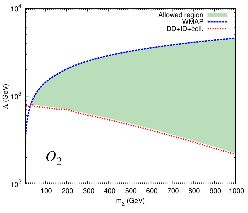
In this section, we do a combined chi-square analysis from all the experimental data sets on each effective operator. Note that the relic density from WMAP7 constrains from above, while all the other experiments constrain from below. Therefore, we combine the chi-squares from (i) direct detection, (ii) collider, (iii) gamma-ray, and (iv) antiproton:
| (58) |
We vary the input parameter until the increase in chi-square is 4 units from the minimum value, i.e.,
| (59) |
The limit on thus obtained is a lower limit. Together with the upper limit due to the WMAP7 data, we show the results for all the operators in Figs. 7, 8, 9, and 10. For each operator there are two curves: one from WMAP7 bounded from above and one from all other experimental data sets bounded from below. We indicate the allowed region by an arrow for each curve. Except for operators , , and , the two arrows in each panel are pointing away from each other, and therefore no region is allowed for all other operators. The working assumption here is that the effective interaction between the DM and SM particles thermalized the DM particles in equilibrium in the early Universe and later decoupled the DM particles according to the standard Boltzmann equation, and there are no other sources for the DM. Under this assumption most of the effective operators, except for , , and , cannot give a smaller interaction constrained by direct detection, indirect detection and collider, while at the same time provide a larger interaction allowed by the WMAP7 data. This is the main result of this work.
Very little parameter space is allowed for most of the operators because we take the assumption that only one operator exists for the early universe and for present day experiments. If there are more than one operators exist at the same time, then the lower limit obtained by all the detection experiments (collider, indirect, and direct) will be stronger; on the other hand, the upper limit due to the relic density will be weaker. Therefore, there would be more allowable regions. Also note that if we further extends to larger masses for in almost all of the operators, there could be some allowed regions.
IX Discussion and Conclusions
Since we have performed the analysis for each experimental data set and the combined analysis, we can easily see which data set dominates for each operator. They are summarized as follows.
- •
dominated by direct detection:
- •
by collider:
- •
by indirect detection ( and -ray):
- •
by collider at low and direct detection at high :
- •
by collider at low and indirect detection at high :
- •
by indirect detection at low and direct detection at high :
The operators , , and that have allowed regions of parameter space are dominantly constrained by the collider data only. This is because these operators in the nonrelativistic limit (e.g. the present Universe) are highly suppressed and thus cannot contribute at any significant level to direct and indirect detection.
In this work, we have exhausted all recent experimental data sets from WMAP7, direct/indirect detection, gamma-ray flux, antiproton flux and collider to obtain important constraints on the effective interactions of the dark matter with the SM particles. We found that almost all effective operators, except for , , and , cannot give a smaller interaction that was constrained by the direct and indirect detection as well as collider data, while at the same time provide a large enough interaction required by the WMAP7 data for the relic density to avoid the Universe over closed by the DM. The result has interesting implications to model buildings, especially those with a heavy mediator between the dark sector and the SM sector. A lot of possibilities shown in this work will not work if we allow at the same time the new physics to give a thermal relic density and to be consistent with the existing data from direct and indirect detections as well as collider data.
Acknowledgments
We thank Eiko Yu and Joel Heinrich for a discussion on treatment of data. This work was supported in parts by the National Science Council of Taiwan under Grant Nos. 99-2112-M-007-005-MY3 and 98-2112-M-001-014-MY3 as well as the WCU program through the KOSEF funded by the MEST (R31-2008-000-10057-0). Y.S.T. is funded by the Welcome Programme of the Foundation for Polish Science.
Appendix A Reductions to effective operators
A.1 Darkon Model
The darkon model [55] consists of a real-scalar boson , which is hidden from the SM interactions, except for a Higgs-portal type interaction with the SM Higgs boson
After the Higgs field develops a VEV , the interactions between the physical Higgs boson and the darkon are given by
such that the interactions of the darkon proceed via the Higgs boson. We can write down the amplitude for as
In the limit , the amplitude becomes
where . This is very similar to the operator in the case of a real scalar DM, with the explicit dependence.
A.2 Higgs Portal model for fermionic DM
The hidden sector consists of a fermion as the DM and a scalar boson , which can mix with the SM Higgs field :
The amplitude for , after boson mixing, is given by
which becomes, in the limit ,
which is exactly the same as with the explicit dependence on .
A.3 - portal model
The hidden sector consists of a fermionic DM and a gauge boson , which then mixes with the SM boson via the kinetic mixing or Stueckelberg-type mixing [56]. The hidden sector does not have any SM interactions originally, but via the mixing with the SM boson, some level of interactions with the SM particles is possible. Suppose the interactions of the DM and the SM fermions are given by, after mixing and integrating out the heavy boson,
then the amplitude for the process can be written as
In the limit of , the amplitude becomes
The couplings of the boson to the SM fermions are all of the same order and the coupling to is unknown, we can, to a crude approximation, take the overall couplings to be similar. Thus, we arrive at the operators to . Note that the coefficients for different SM fermions may as well be different, though they are highly model dependent, they should not differ from one another too much. Again, we take the crude approximation that they are similar and thus reduce a large number of parameters.
A more thorough discussion on deriving various effective operators from various particle exchanges can be found in Ref. [57].
Appendix B Annihilation cross section formulas
Here we list all the differential cross section formulas for the dark matter annihilation of the operators =1 to 20).
| (60) | |||||
| (61) | |||||
| (62) | |||||
| (63) | |||||
| (64) | |||||
| (65) |
| (66) | |||||
| (67) | |||||
| (68) | |||||
| (69) |
| (70) | |||||
| (71) | |||||
| (72) | |||||
| (73) |
| (75) | |||||
| (76) | |||||
| (77) | |||||
| (78) | |||||
| (79) | |||||
| (80) |
where , and are the usual Mandelstam variables, is the cosine of scattering angle, , , , , and is the color factor (3 for quarks and 1 for leptons). We have absorbed the coefficients into in these formulas. The nonrelativistic limits of are listed at the last column of Table 1.
References
- [1] E. Komatsu et al. [WMAP Collaboration], “Seven-Year Wilkinson Microwave Anisotropy Probe (WMAP) Observations: Cosmological Interpretation,” Astrophys. J. Suppl. 192, 18 (2011) [arXiv:1001.4538 [astro-ph.CO]].
- [2] G. Bertone, D. Hooper and J. Silk, “Particle dark matter: Evidence, candidates and constraints,” Phys. Rept. 405, 279 (2005) [arXiv:hep-ph/0404175].
- [3] E. Aprile et al. [XENON100 Collaboration], “Dark Matter Results from 100 Live Days of XENON100 Data,” arXiv:1104.2549 [astro-ph.CO].
- [4] M. Ackermann et al. [The -LAT Collaboration], “Measurement of separate cosmic-ray electron and positron spectra with the Fermi Large Area Telescope,” arXiv:1109.0521 [astro-ph.HE].
- [5] A. A. Abdo et al. [The -LAT Collaboration], “The Spectrum of the Isotropic Diffuse Gamma-Ray Emission Derived From First-Year Fermi Large Area Telescope Data,” Phys. Rev. Lett. 104, 101101 (2010) [arXiv:1002.3603 [astro-ph.HE]].
- [6] Q. -H. Cao, C. -R. Chen, C. S. Li and H. Zhang, “Effective Dark Matter Model: Relic density, CDMS II, Fermi LAT and LHC,” JHEP 1108, 018 (2011) [arXiv:0912.4511 [hep-ph]].
- [7] M. Beltran, D. Hooper, E. W. Kolb, Z. A. C. Krusberg and T. M. P. Tait, “Maverick dark matter at colliders,” JHEP 1009, 037 (2010) [arXiv:1002.4137 [hep-ph]].
- [8] Y. Bai, P. J. Fox and R. Harnik, “The Tevatron at the Frontier of Dark Matter Direct Detection,” JHEP 1012, 048 (2010) [arXiv:1005.3797 [hep-ph]].
- [9] J. Goodman, M. Ibe, A. Rajaraman, W. Shepherd, T. M. P. Tait and H. -B. Yu, “Constraints on Light Majorana dark Matter from Colliders,” Phys. Lett. B 695, 185 (2011) [arXiv:1005.1286 [hep-ph]].
- [10] J. Goodman, M. Ibe, A. Rajaraman, W. Shepherd, T. M. P. Tait and H. -B. Yu, “Constraints on Dark Matter from Colliders,” Phys. Rev. D82, 116010 (2010) [arXiv:1008.1783 [hep-ph]].
- [11] P. J. Fox, R. Harnik, J. Kopp and Y. Tsai, “Missing Energy Signatures of Dark Matter at the LHC,” [arXiv:1109.4398 [hep-ph]].
- [12] A. Rajaraman, W. Shepherd, T. M. P. Tait and A. M. Wijangco, “LHC Bounds on Interactions of Dark Matter,” [arXiv:1108.1196 [hep-ph]].
- [13] K. Cheung, P. Y. Tseng and T. C. Yuan, “Cosmic Antiproton Constraints on Effective Interactions of the Dark Matter,” JCAP 1101, 004 (2011) [arXiv:1011.2310 [hep-ph]].
- [14] K. Cheung, K. Mawatari, E. Senaha, P. Y. Tseng and T. C. Yuan, “The Top Window for Dark Matter,” JHEP 1010, 081 (2010) [arXiv:1009.0618 [hep-ph]].
- [15] K. Cheung, J. Song and P. Y. Tseng, “Cosmic positron and antiproton constraints on the gauge-Higgs Dark Matter,” JCAP 1009, 023 (2010) [arXiv:1007.0282 [hep-ph]].
- [16] C. Boehm, T. Delahaye, P. Salati, F. Staub and R. K. Singh, “Implication of the PAMELA antiproton data for dark matter indirect detection at LHC,” JCAP 1006, 013 (2010) [arXiv:0907.4511 [hep-ph]].
- [17] G. D. Mack, T. D. Jacques, J. F. Beacom, N. F. Bell and H. Yuksel, “Conservative Constraints on Dark Matter Annihilation into Gamma Rays,” Phys. Rev. D 78, 063542 (2008) [arXiv:0803.0157 [astro-ph]].
- [18] P. Scott, J. Conrad, J. Edsjo, L. Bergstrom, C. Farnier and Y. Akrami, “Direct Constraints on Minimal Supersymmetry from -LAT Observations of the Dwarf Galaxy Segue 1,” JCAP 1001, 031 (2010) [arXiv:0909.3300 [astro-ph.CO]].
- [19] D. T. Cumberbatch, Y. L. Tsai and L. Roszkowski, “The impact of propagation uncertainties on the potential Dark Matter contribution to the -LAT mid-latitude gamma-ray data,” Phys. Rev. D 82, 103521 (2010) [arXiv:1003.2808 [astro-ph.HE]].
- [20] J. Goodman, M. Ibe, A. Rajaraman, W. Shepherd, T. M. P. Tait and H. -B. Yu, “Gamma Ray Line Constraints on Effective Theories of Dark Matter,” Nucl. Phys. B844, 55-68 (2011) [arXiv:1009.0008 [hep-ph]].
- [21] D. Hooper and L. Goodenough, “Dark Matter Annihilation in The Galactic Center As Seen by the Fermi Gamma Ray Space Telescope,” Phys. Lett. B 697, 412 (2011) [arXiv:1010.2752 [hep-ph]].
- [22] P. Ciafaloni, M. Cirelli, D. Comelli, A. De Simone, A. Riotto and A. Urbano, “On the Importance of Electroweak Corrections for Majorana Dark Matter Indirect Detection,” arXiv:1104.2996 [hep-ph]; P. Ciafaloni, D. Comelli, A. Riotto, F. Sala, A. Strumia and A. Urbano, “Weak Corrections are Relevant for Dark Matter Indirect Detection,” JCAP 1103, 019 (2011) [arXiv:1009.0224 [hep-ph]].
- [23] N. F. Bell, J. B. Dent, A. J. Galea, T. D. Jacques, L. M. Krauss and T. J. Weiler “ Bremsstrahlung as the Dominant Annihilation Channel for Dark Matter, Revisited,” arXiv:1104.3823 [hep-ph].
- [24] K. Cheung, P. -Y. Tseng and T. -C. Yuan, “Gamma-ray Constraints on Effective Interactions of the Dark Matter,” JCAP 1106, 023 (2011) [arXiv:1104.5329 [hep-ph]].
- [25] J. Fan, M. Reece and L. T. Wang, “Non-relativistic effective theory of dark matter direct detection,” arXiv:1008.1591 [hep-ph].
- [26] J. -M. Zheng, Z. -H. Yu, J. -W. Shao, X. -J. Bi, Z. Li and H. -H. Zhang, “Constraining the interaction strength between dark matter and visible matter: I. fermionic dark matter,” Nucl. Phys. B 854, 350 (2012) [arXiv:1012.2022 [hep-ph]].
- [27] Z. -H. Yu, J. -M. Zheng, X. -J. Bi, Z. Li, D. -X. Yao and H. -H. Zhang, “Constraining the interaction strength between dark matter and visible matter: II. scalar, vector and spin-3/2 dark matter,” arXiv:1112.6052 [hep-ph].
- [28] Ran Ding and Yi Liao “Spin 3/2 Particle as a Dark Matter Candidate: an Effective Field Theory Approach,” arXiv:1201.0506 [hep-ph].
- [29] See for example, K. Cheung, “Collider phenomenology for a few models of extra dimensions,” plenary talk at SUSY2004 [hep-ph/0409028].
- [30] ATLAS Collaboration, “Search for New Phenomena in Monojet plus Missing Transverse Momentum Final States using 1 fb-1 of Collisions at TeV with the ATLAS Detector”, ATLAS-CONF-2011-096.
- [31] T. Aaltonen et al. [ CDF Collaboration ], “Search for large extra dimensions in final states containing one photon or jet and large missing transverse energy produced in collisions at = 1.96-TeV,” Phys. Rev. Lett. 101, 181602 (2008). [arXiv:0807.3132 [hep-ex]].
- [32] E. Carrera [ DØ Collaboration ], “Physics with Single Photons plus Missing Energy Final States at D0,” [arXiv:0906.0041 [hep-ex]].
- [33] DØ Collaboration, “Search for large extra spatial dimensions in Jets + Missing topologies”, DØ CONF-4400 v1.4.
- [34] O. Adriani et al. [ PAMELA Collaboration ], “An anomalous positron abundance in cosmic rays with energies 1.5-100 GeV,” Nature 458, 607-609 (2009) [arXiv:0810.4995 [astro-ph]].
- [35] O. Adriani et al. [PAMELA Collaboration], “PAMELA results on the cosmic-ray antiproton flux from 60 MeV to 180 GeV in kinetic energy,” Phys. Rev. Lett. 105, 121101 (2010) [arXiv:1007.0821 [astro-ph.HE]].
- [36] Z. Ahmed et al. [The CDMS-II Collaboration], “Dark Matter Search Results from the CDMS II Experiment,” Science 327, 1619-1621 (2010) [arXiv:0912.3592 [astro-ph.CO]].
- [37] J. Angle et al. [XENON10 Collaboration], “Limits on spin-dependent WIMP-nucleon cross-sections from the XENON10 experiment,” Phys. Rev. Lett. 101, 091301 (2008) [arXiv:0805.2939 [astro-ph]].
- [38] V. N. Lebedenko et al. [ZEPLIN-III Collaboration], “Limits on the spin-dependent WIMP-nucleon cross-sections from the first science run of the ZEPLIN-III experiment,” Phys. Rev. Lett. 103, 151302 (2009) [arXiv:0901.4348 [hep-ex]].
- [39] M. Felizardo et al. [SIMPLE Collaboration], “Final Analysis and Results of the Phase II SIMPLE Dark Matter Search,” arXiv:1106.3014 [Astro-ph.CO].
- [40] A. Friedland, M. L. Graesser, I. M. Shoemaker and L. Vecchi, “Probing Nonstandard Standard Model Backgrounds with LHC Monojets,” arXiv:1111.5331 [hep-ph].
- [41] I. M. Shoemaker and L. Vecchi, “Unitarity and Monojet Bounds on Models for DAMA, CoGeNT, and CRESST-II,” arXiv:1112.5457 [hep-ph].
- [42] Y. Mambrini and B. Zaldivar, “When LEP and Tevatron combined with WMAP and XENON100 shed light on the nature of Dark Matter,” JCAP 1110, 023 (2011) [arXiv:1106.4819 [hep-ph]].
- [43] A. Kurylov and M. Kamionkowski, “Generalized analysis of weakly interacting massive particle searches,” Phys. Rev. D 69, 063503 (2004) [hep-ph/0307185].
- [44] C. E. Aalseth et al. [ CoGeNT Collaboration ], “Results from a Search for Light-Mass Dark Matter with a P-type Point Contact Germanium Detector,” Phys. Rev. Lett. 106, 131301 (2011) [arXiv:1002.4703 [astro-ph.CO]].
- [45] R. Bernabei et al. [ DAMA Collaboration ], “First results from DAMA/LIBRA and the combined results with DAMA/NaI,” Eur. Phys. J. C56, 333-355 (2008) [arXiv:0804.2741 [astro-ph]].
- [46] P. Gondolo, J. Edsjo, P. Ullio, L. Bergstrom, M. Schelke and E. A. Baltz, JCAP 0407, 008 (2004) [arXiv:astro-ph/0406204].
- [47] H. -Y. Cheng and C. -W. Chiang, arXiv:1202.1292 [hep-ph].
- [48] J. Engel, S. Pittel and P. Vogel, “Nuclear physics of dark matter detection,” Int. J. Mod. Phys. E 1, 1 (1992).
- [49] J. A. M. Vermaseren, “New features of FORM”, math-ph/0010025.
- [50] P. J. Fox, R. Harnik, J. Kopp and Y. Tsai, Phys. Rev. D 84, 014028 (2011) [arXiv:1103.0240 [hep-ph]].
- [51] A. W. Strong, I. V. Moskalenko, T. A. Porter, G. Johannesson, E. Orlando and S. W. Digel, “The GALPROP Cosmic-Ray Propagation Code,” arXiv:0907.0559 [astro-ph.HE].
- [52] R. Trotta, G. Johannesson, I. V. Moskalenko, T. A. Porter, R. R. de Austri and A. W. Strong, “Constraints on cosmic-ray propagation models from a global Bayesian analysis,” Astrophys. J. 729, 106 (2011) [arXiv:1011.0037 [astro-ph.HE]].
- [53] T. Sjostrand, S. Mrenna and P. Z. Skands, “A Brief Introduction to PYTHIA 8.1,” Comput. Phys. Commun. 178, 852-867 (2008) [arXiv:0710.3820 [hep-ph]].
- [54] M. Ackermann et al. [Fermi-LAT Collaboration], Phys. Rev. Lett. 107, 241302 (2011) [arXiv:1108.3546 [astro-ph.HE]].
- [55] X. -G. He, T. Li, X. -Q. Li, J. Tandean and H. -C. Tsai, “Constraints on Scalar Dark Matter from Direct Experimental Searches,” Phys. Rev. D 79, 023521 (2009) [arXiv:0811.0658 [hep-ph]].
- [56] K. Cheung and T. -C. Yuan, “Hidden fermion as milli-charged dark matter in Stueckelberg Z- prime model,” JHEP 0703, 120 (2007) [hep-ph/0701107].
- [57] P. Agrawal, Z. Chacko, C. Kilic and R. K. Mishra, “A Classification of Dark Matter Candidates with Primarily Spin-Dependent Interactions with Matter,” arXiv:1003.1912 [hep-ph].