Quantum coherent control of highly multipartite continuous-variable entangled states by tailoring parametric interactions
Abstract
The generation of continuous-variable multipartite entangled states is important for several protocols of quantum information processing and communication, such as one-way quantum computation or controlled dense coding. In this article we theoretically show that multimode optical parametric oscillators can produce a great variety of such states by an appropriate control of the parametric interaction, what we accomplish by tailoring either the spatio-temporal shape of the pump, or the geometry of the nonlinear medium. Specific examples involving currently available optical parametric oscillators are given, hence showing that our ideas are within reach of present technology.
pacs
42.50.Dv–Quantum state engineering and measurement, 42.65.Yj–Optical parametric oscillators and amplifiers, 42.65.Re–Ultrafast processes, optical pulse generation and pulse compression.I Introduction
Squeezed states of light were introduced several decades ago as states which could help beating the limits set by quantum mechanics on the precision of measurements performed with coherent light [1, 2]. These are states in which one of the quadratures of light (equivalent to the position and momentum of a mechanical oscillator) has a quantum uncertainty below the vacuum or “shot noise” level, at the expense of increasing the quantum fluctuations in the orthogonal quadrature. These states found their way into the new century thanks to their widely proved applications in ultra-precise metrology (such as gravitational wave detection [3, 4] or beam displacements [5, 6]), as well as in the field of quantum information with continuous variables [7, 8], where the highest-quality entangled states (the basic ingredient of many quantum information protocols) known to date are currently obtained by mixing squeezed beams with linear optics [9, 10].
Squeezed light can be obtained via the parametric down-conversion process that takes place inside a second order nonlinear medium pumped by a laser beam [1]. In order to increase the nonlinear interaction, it is customary to insert the nonlinear crystal in an optical cavity—dealing then with a so-called “optical parametric oscillator” (OPO)—, and large levels of squeezing are obtained in the down-converted field when the OPO is operated close to threshold, 93% of noise reduction being the current benchmark [11] (see also [12, 13]).
On the other hand, quantum information has reached a stage where real-world applications stimulate an intense research for the implementation of reliable and practical quantum protocols for quantum communication and information processing. Several of the promised benefits require though a quantum “substrate” that is created by distributing quantum correlations (entanglement) among a number of degrees of freedom (modes) increasing with the complexity of the task to achieve. The protocols of quantum telecloning [14, 15] and controlled dense coding [16, 17] constitute paradigmatic examples of this scenario for small number of modes, while one-way quantum computation [18, 19, 20, 21], in which the computation is achieved by applying local measurements to a set of modes initially in a cluster state, is a most promising example in the large number of modes regime.
However, the generation of such multipartite entangled states by means of optical devices requires experimental configurations whose complexity increases with the number of modes involved [10, 17, 22, 23, 24, 25]. In contrast, a practical source should be compact, scalable, and permit to master the quantum properties of the generated states even when the number of modes is very large.
A continuous-variable cluster state source with these properties was proposed in [26]—and refined in subsequent papers [27, 28] (see also [20])—, which consisted in an OPO driven by a multifrequency pump field in the presence of concurrent nonlinearities. Recently, these ideas have been brought to the laboratory, and the record of 15 quadripartite cluster states have been generated along 60 consecutive longitudinal modes of the OPO cavity [29]. This interesting approach is however limited by the number of frequencies that can be coupled within the phase-matching bandwidth, the need of frequency-sensitive measurements, and the fact that a nonlinear crystal with different phase-matching properties has to be engineered for each particular cluster state that one desires to create. An even more simple and promising approach based on the synchronously operation of only one single mode vacuum squeezer and a quantum non-demolition gate was proposed very recently in [30].
In this paper we propose an alternative approach based on the use of a naturally multimode optical parametric oscillator, either in the spatial [31, 32, 33, 34, 35, 36, 37, 38, 39, 40, 41, 42] or in the temporal domain [43, 44]. Below threshold, they produce multimode squeezed states, which has been observed experimentally [42, 45]. When operated above threshold, such multimode devices have been recently proved to be capable of producing non-critically squeezed states of light via the phenomena of spontaneous symmetry breaking [32, 33, 35, 41, 46] and pump clamping [37, 42].
The advantage of the scheme introduced in the current article for the generation of cluster states over previous proposals [20, 26, 27, 28] is that one does not need to engineer the couplings between each mode through crystal design (which is specific of each coupling scheme): choosing instead the temporal or spatial shape of the pump (which is a flexible technique) is enough to directly control the characteristics of the generated quantum state, even for a very large number of modes. We will show that it is possible to master in this way the number of entangled modes, as well as the distribution of their quantum correlations, thus permitting the generation of arbitrary multimode Gaussian quantum states of any dimension. The technique that we propose is therefore reminiscent of the widely used “coherent control” of evolution of atoms and molecules that is obtained by appropriately shaping the pulses with which they interact [47, 48].
The article is organized as follows. In Section II we show how both the light generated via single-pass spontaneous parametric down conversion in the low-gain regime, as well as that leaving a multimode optical parametric oscillator below threshold, can be described as a combination of independent, squeezed modes (termed “supermodes” later on). After considering a particular (but physically relevant) example of the parametric interaction to show how these supermodes arise (Section III), we demonstrate that the squeezing and spatio-temporal shape of such modes can be controlled either by tailoring the shape of the pumping field, or the geometry of the nonlinear medium; we consider separately the cases of an OPO with either many longitudinal modes (Section IV.1) or just a few transverse modes (Section IV.2) available for parametric down-conversion. We then explain how our results can be used for the generation of arbitrary cluster states of copropagating modes in Section V, and give our conclusions in Section VI.
II Generalized supermode description of weak parametric interactions
The dynamics of parametric interactions in the low-gain regime (for single-pass devices) or below its oscillation threshold (for cavity devices) is controlled by a kernel function or matrix (depending on the continuum or discrete nature of the modes involved) which describes the coupling among the different relevant signal-idler modes. As shown in previous studies, the diagonalization of such kernel is instrumental for determining the objects with well-defined quantum properties, which turn out to be linear combinations of the signal-idler modes. Such linear combinations were termed “supermodes” in [43] and the next subsections are devoted to their introduction in both single-pass and cavity devices. We will consider collinear type I degenerate phase matching for definiteness but our treatment can be generalized easily to other types of phase matching.
II.1 Single-pass parametric interactions
In the single-pass configuration the pump beam amplifies parametrically the quantum noise impinging the crystal around the subharmonic frequencies and the down-converted field is measured at the exit of that crystal. In the undepleted pump approximation, holding when parametric gain is low, the “output” boson operators are generically related to the “input” ones via the well known Bogoliubov transformation
| (1) |
where is a general continuous index standing for frequency or/and transverse position11 1 Transverse means orthogonal with respect to a propagation direction, in which case the paraxial approximation is assumed., and and are Green functions that solve the propagation equations (see [49] for details). In the very weak conversion limit a perturbative treatment can be applied to first order in the crystal length, which physically means considering only generation of single photon pairs. In such case and , where is a coupling constant proportional to the length and nonlinear susceptibility of the crystal and to the square root of the total pump irradiance , and is a kernel. Hence in this regime (1) becomes
| (2) |
As we will see immediately, the form of is universal, and is given by the product of the pump amplitude and some function describing the overlap between modes over the crystal. However, the special form of depends on the considered problem and in the following we treat successively the temporal and spatial aspects of single-pass parametric interaction in the single photon pair approximation (2).
Let us begin by the spectral/temporal aspects in which case corresponds to the frequency of the monochromatic modes (we call this the temporal case). Assuming that all the parametrically coupled modes have the same transverse dependence, and neglecting diffraction inside the crystal, the coupling kernel turns out to be [49]
| (3) |
being proportional to the spectral pump amplitude at frequency , and the usual phase-matching function22 2 In [49] a factor is included in the expression (4). Here it is absent because we are implicitly working in the interaction picture with respect to time and space, analogous to Eq. () in [49], see [43, 44] for details.
| (4) |
where , is the optical wavenumber at frequency inside the crystal, is the sinus cardinal function, and
| (5) |
is a phase mismatch.
Let us now turn to the spatial case within the paraxial approximation, in which case is the transverse spatial variable (). We define this “spatial case” in the sense that pump is assumed monochromatic and focus is put on the signal/idler (multimode) field at just the subharmonic frequency, in which case the kernel is given by [40]:
| (6) |
being the normalized pump amplitude at transverse point , and the diffraction function
| (7) | |||||
being the phase-matched signal wavenumber inside the crystal, the “coherence length”, and the sine integral function.
In the general case, the spatial and spectral aspects of the parametric interaction are simultaneously present, giving rise to new interesting features [50] which we will not consider here.
II.2 Intracavity parametric interactions
When an optical cavity is used to enhance the efficiency of the nonlinear process, the previous nonlinear couplings represented by kernel are projected onto the cavity modes, and the multi-dimensional spectral and spatial properties of the correlated photons can be lost due to such filtering. However for a given length and geometry of the cavity, which we assume to have a cylindrical symmetry around the optical axis, a great number of modes can be simultaneously sustained: in the frequency domain they are the series of longitudinal modes separated by the free spectral range of the cavity; in the transverse spatial domain they are the set of Laguerre-Gauss modes .
In the temporal case we assume the pump consisting of an unlimited series of pulses at a given repetition rate, equal to the free spectral range of the cavity: this is what is called a Synchronously Pumped OPO (SPOPO) [43, 44]. The pump spectrum is thus a frequency comb, consisting of a large number of frequency components, each of which gives rise to signal-idler photons belonging to different longitudinal modes through the parametric down conversion process, and selected by energy and linear momentum conservation.
In the spatial case, on the contrary, the pump is assumed monochromatic with a given spatial profile. In this case, owing to the linearity of the interaction in the below threshold regime, one can focus on, say, the subharmonic signal photons. However these photons belong, in general, to different transverse modes (degenerate in frequency), characterized by a constant value of the sum , known as “family index” [37]. As well, even several families of transverse modes can become relevant in the case of a degenerate cavity such as the the confocal [31, 34, 51] or the self-imaging cavity [40, 52], in which many different families (with different family indices ) resonate at the same frequency. We will use a single generic index to label this discrete series of modes.
It is instructive in this intracavity interaction problem to write down the interaction Hamiltonian in the undepleted pump approximation, which can be written in general as
| (8) |
where the continuous boson operators satisfy the standard commutation relations
| (9a) | |||||
| (9b) | |||||
and the kernel plays a role analogous to that in single-pass devices.
In the temporal/spectral case (SPOPO) the Hamiltonian of the nonlinear interaction can be written in terms of discrete creation and annihilation operators of the cavity longitudinal modes:
| (10) |
where are the specialization of the continuous-variable kernel (3–5) to the relevant longitudinal modes around the subharmonic, and is the boson operator for the signal-idler mode verifying . The dynamics of the intracavity modes is then given by the following quantum Langevin equations
| (11) |
where is the cavity loss rate (assumed identical for all signal/idler modes – which, by the way, cannot be distinguished from one another in this collinear type I degenerate phase matching case), and is a dimensionless pumping parameter proportional to the actual pump power (see, e.g. [44] for more details).
In the spatial case (as defined in the previous Section), under circumstances in which only a few signal modes are relevant [37], Hamiltonian (10) holds by identifying the indices with the available TEMpl modes at the signal frequency, whose dynamics are ruled by the quantum Langevin equations (11). In degenerate cavities, such as confocal or self-imaging cavities, a discrete representation is still possible, but a continuous one (8) is more helpful, in which case the quantum Langevin equations become [40]
| (12) |
For self-imaging cavities [40] the kernel is given by (6) and (7), while for the confocal case it has a slightly different expression [31] owed to the fact that even and odd transverse families resonate at different frequencies.
II.3 Supermodes
We have seen in the previous Section that the output from parametric devices in the low-gain (or below threshold) regime is governed by a kernel , which is equal, under equivalent conditions, in the single-pass and intracavity cases. As both the input-output relations in single-pass configurations and quantum Langevin equations in cavity devices are linear in the considered regime, diagonalization of the kernel allows a considerable simplification in the description of the problem as well as a clear physical picture of the entities in which clean quantum properties are concentrated. This approach [40, 43, 44, 49] is the single-partite and continuous-variable version [53] of the Schmidt decomposition for the bi-partite bi-photon wave function [54], which in general is formally expressed by the Bloch-Messiah decomposition [55].
Let us introduce the eigenmodes of the continuous kernel , which are the solutions of the Fredholm integral equation:
| (13) |
Starting from the eigenmodes , we can define the associated supermode annihilation operator as
| (14) |
where we assume to be normalized so that . These operators annihilate a photon in a mode which is a combination of either spatial or frequency modes, and we call it “supermode” [43] because it is the combination of many cavity modes and has a non trivial spatial or spectral/temporal shape in general. Using (14) and (13) into Eq. (2) we get
| (15) |
When the crystal is inserted in an optical cavity—OPO case—, Ref. [43] shows that the supermodes can be defined as a discrete combination of the cavity eigenmodes instead of the continuous combination written above, corresponding to the diagonalization of matrix in Eq. (11). These two possible expressions are identical in the limit where the cavity modes are tight enough so that the sum can be assimilated to an integral. In the following we assume that this condition is fulfilled. In this case, the evolution of these supermode operators is governed by a set of uncoupled quantum Langevin equations obtained by introducing the discrete versions of (14) and (13) in Eq. (11):
| (16) |
This equation shows that according to this definition, any multimode OPO can be in fact seen as a set of independent single-mode OPOs, and therefore can produce a set of copropagating squeezed supermodes. Hence each supermode is independently squeezed, and the squeezed quadrature can be shown to have a noise level at zero frequency equal to ( setting the shot-noise level) when the system is operated close to threshold, where is the eigenvalue of largest absolute value.
III A general method for tailoring the supermode spectrum
The solution of Eq. (13) is simple when the kernel factorizes,
| (17) |
in which case the unique eigenmode is, within a multiplicative factor, , with corresponding eigenvalue . This result can be extended to the case where there is a set of orthogonal functions such that
| (18) |
in which case Eq. (13) has solutions (save multiplicative constant), . When has the same type of decomposition as (18), but with non orthogonal functions, just linearly independent, one can show that (13) has still solutions [56], which are now different from the functions .
The analytical description of the kernel in terms of a basis of linearly independent functions (supermodes) like in Eq. (18) has a very simple solution and physical interpretation in the case where the kernel can be factorized as
| (19) |
In the spatial case this is the form encountered [40], see (6): relates to the pump, while has to do with the crystal. In the temporal case, while this is not the most general kernel one can find in actual applications, it has been shown in [44, 49] that it is a sensible approximation to many real cases. The function in (19) can be manipulated by tailoring the pump shape, while in order to tune the function one needs to play with the geometry of the nonlinear crystal.
We now exhibit a series of “simple” kernels which allow a high degree of control over their spectra and, as we will show in the next Section, find applications in actual systems.
Let us start by the simplest case, the symmetric Gaussian kernel, defined by , reading
| (20) |
as in (17), whose only supermode is the Gaussian function , with corresponding eigenvalue .

Let us now consider the previous symmetric kernel (20), now multiplied by cosine functions of and , i.e.:
| (21) |
which is a quasiperiodic modulation of the Gaussian kernel. In (21), are constants and by definition. This leads to a kernel (19) which can be written like in Eq. (18)—with non-orthogonal functions —using well known trigonometric formulae. We have therefore shown that a kernel having the form (19) with (21) will have exactly eigenmodes, or modes if the constant terms . As shown in Appendix A a simple way to diagonalize the kernel defined by (21) consists in using auxiliary functions
| (22) |
where stands for any of the trigonometric functions or , in terms of which actual eigenvectors and eigenvalues can be found by linear combinations of them. The expressions for eigenvalues and eigenvectors are awfully cumbersome but one can show that whenever
| (23) |
the functions (22) are approximate eigenvectors indeed. For each couple in (22) two doubly degenerate eigenvalues are found, of equal magnitude but opposite sign: . The positive one is associated to and the negative one to . As for the cases and , in which and respectively, the eigenvalues read and , respectively. Finally, the eigenvalue associated to the fundamental Gaussian eigenvector, that is, to the case , reads .
We have therefore shown that one is able to master the number of supermodes and the magnitude and sign of their eigenvalues by a proper choice of the modulation amplitudes of the parametric multimode interaction kernel (21). In Figure 1 we give two examples of kernels, designed so as to lead to eigenvalues respectively proportional to and . We note that the results shown in the figures have been obtained by numerically diagonalizing the kernels, what gives additional support to our previous approximate analytical treatment.
Our analysis has been restricted so far to the case of kernels with symmetric Gaussians. However, it can be readily extended to the more physical case of a kernel factorizing in two Gaussian functions of variables and having unequal widths [44, 49]. In fact this is the most general situation as it is not always possible to configure the OPO/OPA in such a symmetric way (in SPOPOs, for instance, for typical situations one has a difference of one order of magnitude between Gaussian widths). In this case the kernel we propose has again the factorized form (19), now with
| (24) |
instead of (21), where we allowed for different widths, , along the directions and . In Appendix B we give the eigenvalues and eigenvectors of this general case.
IV Controlling the number of supermodes and the eigenvalues in actual parametric devices
The method we sketched out above can be practically applied to spatial or temporal modes of the OPO/OPA since in both cases a factorized form (19) of the kernel is a very good approximation (it is even exact in the “spatial case”), and both admit as well an approximated Gaussian form, see e.g. [44, 49, 53]. The point is then how to implement in real devices the quasiperiodic modulations we introduced in the previous Section.
We will divide our presentation in two Subsections. The first one deals with what we call the continuous case, which includes both problems in which a continuous boson representation is used (single-pass devices) or problems in which, being that representation discrete, the kernel can be treated as a continuous function (SPOPO [44] and the self-imaging OPO [40]). The second Subsection deals with what we call the discrete case, in which a discrete boson representation is used and a discrete treatment of the problem is simpler, given the relatively small number of modes involved, like an OPO tuned to a single transverse mode family [37].
IV.1 The continuous case
As for the Gaussian form of the subkernels we note that both the phase-matching function (4,5) of the temporal case and the diffraction function (7) of the spatial case can be well approximated by the Gaussian . In the temporal case [44, 49]
| (25) |
being the derivatives of the pump/signal wavenumber with respect to frequency at phase matching, while in the spatial case . Hence if the pump spectral amplitude has a Gaussian shape , being the individual pulse duration, the total kernel can be approximated by with . If the pump has not a Gaussian shape but can be expressed as a sum over functions, (hence ) and the Gaussian kernel will be multiplied by those modulations (see below).
As the pump amplitude is a factor of , see Eq. (3), a simple and practical way to tailor the kernel is by shaping the pump, as we will see more precisely now.
IV.1.1 Tailoring the pump
We focus on the temporal case [43, 44, 49] and hence deal with pumps consisting of pulses. However the ideas put forward below can be applied equally to the spatial case [40] by substituting the pulse shapers we consider by amplitude masks or simply by superposing different plane waves.
Using pulse shapers with harmonic spectral response:
A first possible method consists of using a pulse shaper [57] with several well separated amplitude modulations on the Spatial Light Modulator (SLM). The effect of such pulse shaper in the frequency domain can be represented in the general case by the modulating function
| (26) |
where by definition. The incoming pump field, of temporal envelope , is sent onto a diffraction grating and the image is created in the Fourier plane of a lens in correspondence of the SLM mask. Immediately after the mask, the outgoing field has a spectrum . Then another lens and diffraction gratings perform the inverse Fourier transform so that the outgoing field has the following temporal shape: , i.e. the usual convolution, which is used to pump the SPOPO. It is then straightforward to see that, by using in Eq. (3), one obtains a modulation of the kernel as in Eq. (24), with , and . As a consequence, the eigenvalues are proportional to according to the analytical solutions given in Section III.
Using pulse shapers leading to special waveforms:
In this case we assume that a pulse shaper has been programmed so as to convert the frequency comb coming from the pumping laser (whatever its temporal waveform could be) into into a sequence of equal rectangular pulses at the frequency comb repetition rate. Hence the pump spectrum is proportional to , being the pulse duration. Then, if is much smaller than the width of the crystal response function along the direction —equal to defined in Eq. (25)—, i.e. for “long” pulses, the kernel can be approximated by , see Eq. (3), where [44]. As a consequence, as can be approximated by a finite (Fourier) sum of functions , with large as compared to , the kernel reads as in (24). As the coefficients of the Fourier series, , are all very similar (because of the function , whose Fourier transform is rectangular) we expect a large degree of degeneracy between eigenmodes, as is actually evidenced by numerically diagonalizing the corresponding kernel.
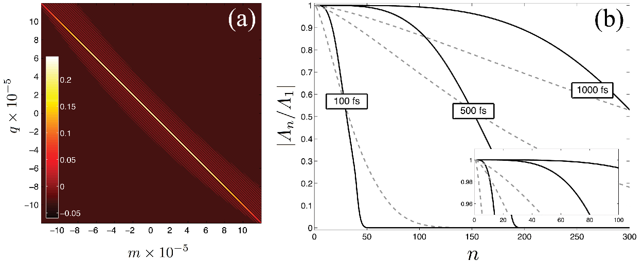
In Figure 2a we trace the kernel corresponding to a realistic situation where a SOPO cavity, with the nonlinearity of a 100-thick BIBO crystal (fs; see [44] for details), is pumped by a train of square pulses. The eigenvalues obtained by the numerical diagonalization of for increasing values of are shown in Figure 2b and are compared with the corresponding cases of Gaussian pump pulses: as expected, the degree of degeneracy increases dramatically with the duration of the square pump pulses. For instance, for pulses the first hundred eigenvalues differ by less than 1%, see the inset in Figure 2b, what allows the generation of very high quality, highly multi-dimensional entanglement.
Using delay lines
A third method consists in using delay lines that, starting from one comb, allow the superposition of several combs so that each “tooth” in the temporal domain is made of a series of pulses delayed/advanced by with respect to the first one; one then gets as many eigenvalues as there are different superposed combs, the eigenvalues being proportional to the amplitude of each comb as we show next. For example, being the (normalized) envelope of the pump field associated to a train of pulses incoming the OPA or the SPOPO cavity, the envelope of the pump field associated to a generic superposition of delayed/advanced trains of pulses reads
| (27) |
where and are real coefficients controllable in the experiment. In the Fourier domain Eq. (27) reads
| (28) |
being the Fourier transform of . Since we have the same eigenproblem as in the previous cases, the eigenvalues will be again proportional to .
IV.1.2 Tailoring the crystal response
Another interesting possibility in the temporal case is to modify not the pump temporal shape but the effect of the nonlinear medium, which allows us to control the function . It can be accomplished by using several identical non-linear crystals which are not perfectly phase-matched and separated by fixed distances. In the general case where crystals of thickness are used, centered at planes , the corresponding phase-matching function , see (4), reads
| (29) | |||||
where is given in (5). If the crystals are arranged symmetrically by couples at distances between mid-planes, then the above expression becomes
| (30) |
where now the sum extends over couples of crystals33 3 If the number of crystals is odd, say , then Eq. (30) is modified by substituting the sum upper limit by , and adding a term equal to to the result, as can be easily checked.. When the pump spectrum is narrow as compared with the width of along the direction —the quantity defined in Eq. (25)—a safe approximation consists in setting in . Hence,
acts as a harmonic modulation (equivalent to , , , and in our previous notation) of the single-crystal kernel, and the latter can be approximated by a factorized Gaussian form as already discussed, so the full kernel takes the form (24).
IV.2 Discrete case
As commented in Section II.2, the discrete representation is useful when dealing a low number of signal modes. A typical configuration corresponding to this case is given by OPO with monochromatic pump, whose cavity is tuned at the subharmonic to some transverse mode family represented by the family index [37]. Recall that family contains the Laguerre-Gauss modes with , being equal to for even families and for odd families.
In order to simplify the upcoming discussion, we assume that the the pump beam has a coaxial cylindrical symmetry, in which case Orbital Angular Momentum (OAM) conservation ensures that the down-converted photons must have opposite OAMs. This implies that, if one uses the basis of Laguerre-Gauss modes , the parametric down-conversion Hamiltonian takes the form [37]
| (31) |
with
| (32) |
and being the transverse profiles of the (normalized) pump field and the Laguerre-Gauss modes 44 4 Explicitly, we have (33) where are the modified Laguerre polynomials and is the spot size of the beam at the cavity waist. at the cavity waist, respectively, and the creation operator associated to the Laguerre-Gauss mode , which we abbreviate as from now on because a fixed value of the family index is assumed as explained.
The continuous boson operators defined on the transverse plane can be expressed in terms of Laguerre-Gauss modal operators as
| (34) |
The kernel of Hamiltonian (8) has therefore the following expression:
| (35) |
This expression is close to the one assumed in (19). It can actually be brought to that exact form by introducing the Hybrid Laguerre-Gauss modes
| (36a) | |||||
| (36b) | |||||
which are respectively proportional to and . The kernel can then be written as
| (37) |
In other words, we have just shown that the Hybrid Laguerre-Gauss modes and are the supermodes for the present OPO configuration. In addition, both the “sine” and “cosine” type modes have the same eigenvalue (). Note that nothing prevents from being complex, say , what means that the supermodes with different can be squeezed along different directions of phase space, direction in particular for modes . As for the number of available supermodes , it is given by the number of modes contained in family , that is, .

Let us now consider the situation in which the pump has a Gaussian shape, that is, , where
| (38) |
is a TEM00 mode with spot size , being the spot size of the transverse modes at the signal frequency and a scaling factor (the factor in is included for dimensional reasons, as we defined as a dimensionless, normalized pump amplitude). It is obvious from (32) that ; in other words, the lower the OAM, the better the signal modes overlap with the pump profile. However, for a large enough , the pump profile is somehow seen as plane by all the signal modes, and the couplings become independent of :
| (39) |
Hence, by pumping with a wide Gaussian, one can bring all the couplings to a common value, at the expense of decreasing them, hence increasing the OPO threshold. Note however that, as discussed next, the desired effect is obtained even for moderate values of , so that the OPO threshold stays within reasonable limits.
In Fig. 3 we show the ratios as a function of for the first families. Note that the axis starts at , which is the value one has in the doubly resonant configuration (cavity resonant both for the signal and the pump). Note also how goes very quickly above , which is the value above which one finds more than 90% squeezing for the corresponding supermodes [37]. In the insets, we show which gives the ratio between the pump power needed to make the signal field oscillate for a given and that for ; note that the threshold is not dramatically increased for reasonable values of (it is even decreased for small ).
One can even tune the actual values of the couplings to specific values by pumping not with a single TEM00 mode, but with a combination of TEM00 modes of different widths. To show this, let us consider two examples within the third family of transverse modes (, and then ). First, we want to make , so that the eigenvalues of the supermodes have the same magnitude, but opposite sign. In this case, we can use the following pump profile
| (40) |
that is, a superposition of two Gaussians with opposite phase, and spot sizes and . Note that this type of pump shape can be easily obtained in the lab by mixing the Gaussian beams on a beam splitter. It is then straightforward to show that choosing the mixing angle such that
| (41) |
one gets . Note that, in the general case where the resonator is tuned to family , one can have complete control of all the ratios between the coupling parameters by using TEM00 beams with adjustable amplitudes as pumping beams.
In the second example we show the very interesting case where some of the couplings become zero by using an appropriate pump shape. To show that this extreme case is indeed possible, we consider the previous example with the following choice of the mixing angle between the Gaussians:
| (42) |
in which case it is simple to show that , while can be large enough with a proper election of . It can be interesting, for example, to choose the mixing angle between the Gaussians in order to cancel the coupling with the TEM00 modes in a general OPO, so as to favor the coupling to the TEM10/01 modes, thus forcing it to emit the signal and idler modes with opposite OAM. This way, one can induce a spontaneous breaking of the radial symmetry, what has been predicted to give rise to some remarkable quantum properties [35, 41].
The methods discussed so far allow us to tune at will the eigenvalues of the supermodes, but not the spatial profile of the supermodes themselves (they are the Hybrid Laguerre-Gauss modes in all the cases). In order to change the form of the supermodes, we can go a little further and add beams with non-zero OAM to the pump, what would allow us to engineer any kind of coupling between the modes with definite OAM of a given family. For example, if one uses a pump field with a OAM component, it becomes possible to couple the signal modes with and OAM; mixing several of these pump beams, one can even tune each of these couplings to a desired complex value, so much as we have shown for the couplings between the signal modes with OAM by pumping with zero OAM Gaussian beams.
V Application to the generation of arbitrary cluster states
Having a set of copropagating modes with squeezing properties chosen at will (as we have discussed along the previous sections) offers the possibility of generating any type of continuous-variable cluster state, that is, of producing any type of Gaussian multipartite entangled state. To see this, just note that we have proved that these modes, which we have called supermodes, evolve according to the Hamiltonian
| (43) |
where is the creation operator associated to the supermode of the kernel having eigenvalue , both of which can be controlled via any of the ideas explained in the previous section. Note that this Hamiltonian can be written as
| (44) |
where is a row vector operator, superscript “” denotes transposition, and we have defined the diagonal matrix . Through an arbitrary unitary matrix , we can define a set of creation operators for some new modes, so that
| (45) |
where is a new coupling matrix. Hence (43) can be seen as the diagonal form of (45). For each choice of the coupling matrix , which can be chosen as symmetric without loss of generality, this Hamiltonian generates a different type of multipartite entanglement between the modes.

As simple examples, consider the cluster states represented in Figure 4. In the first type, four modes of a circle are connected (all with same strength) only to their first-neighbors, one coupling having opposite sign respect to the rest. The corresponding coupling matrix is (appart from a multiplicative factor)
| (46) |
which has doubly degenerate eigenvalues . Note that these eigenvalues correspond exactly to some of the examples considered in previous sections, in particular, to the example shown in Figure 1a of Section III, and to the second example of the previous section, where the couplings and of an OPO tuned tuned to the third family of transverse modes were tuned to the same absolute value and opposite sign.
In the second example of Figure 4, five modes are interconnected with the same strength via the coupling matrix (again appart from a possible multiplicative factor)
| (47) |
which has eigenvalues coinciding with the example of Figure 1b in Section III. In the discrete spatial case, these eigenvalues can be obtained by tuning the resonator to the family of transverse modes and tuning the couplings to , which can be done via the multi-Gaussian pump technique discussed in the previous section, in this case with Gaussians of appropriate widths and weights.
Incidentally, we note that these two cluster states are of very different nature: while in the first case tracing out one of the modes does not destroy the bipartite entanglement shared between the rest of the modes, this is not the case in the second example, in which tracing out one of the modes leads to a completely separable state. In the latter case, we then say that the entanglement is “genuinely multipartite” [7].
Indeed, the state of the second example in Figure 4 corresponds to the class of so-called GHZ-like states [7], that is, states which tend to
| (48) |
in the limit of perfect squeezing (kind of generalization of EPR states to modes), and are then completely characterized by the variance of the joint quadratures and , being and [7, 58], of which is indeed an eigenstate.

There is another way of obtaining GHZ-like states from a set of squeezed modes , which was introduced by van Loock and Braunstein [10], who proposed to start from modes squeezed along a given direction of phase space, plus another one squeezed along the orthogonal direction—a state that can be produced in the way explained in the present paper—, and to apply to this state a specific transformation known as the so-called “Braunstein rotation” [59, 10].
Note that in order to have a reasonable approximation of the GHZ state, one needs large squeezing in all the initial modes. In the previous section we actually showed that by pumping with a wide enough Gaussian mode an OPO tuned to the -th family of transverse modes, one can bring together the thresholds of the modes contained in that family, and hence all the supermodes will leave the OPO highly squeezed when working close to threshold. Note however that all the supermodes are squeezed in their quadrature (taking the pump phase as the reference), and hence, before applying Braunstein’s rotation, one needs to perform a phase shift in one of them to obtain the true entangled modes. In Figure 5 we show the transverse profile (square modulus) of these modes for the first families (the phase shift has been applied to the supermode). Note that using SPOPOs pumped by rectangular pulses we showed that one can generate hundreds of highly squeezed supermodes (see Figure 2), and hence, this system offers a highly dimensional alternative to the OPO tuned to a given transverse family where the number of squeezed supermodes is more modest.
VI Conclusions
We have shown that an appropriate shaping of the pump beam (or of the geometry of the nonlinear medium) enables us to generate in a multimode OPO any Hamiltonian bilinear in the annihilation operators of the down-converted modes, and therefore to generate highly multimode non-classical states of light that may be of interest. In addition, we have shown that these quantum states are easily characterized in a special mode basis, the basis of “supermodes”, as a superposition of independent, squeezed copropagating modes.
The measurement of the quadrature components of any mode is always possible with a balanced homodyne set-up using a coherent state in the mode of interest as a local oscillator, which projects the multimode state on the mode of the local oscillator. However, this technique is destructive, so that it allows for a measurement of the properties of one supermode at a time. An alternative to this single-mode homodyne detection is multiplexed homodyne detection [60, 39], with which it is possible to recover simultaneous information of the different supermodes using an appropriate data processing protocol. This opens the possibility of considering the copropagating entangled modes as a valid resource for one-way quantum computation, at least in the Gaussian domain.
Even though having a cluster state between copropagating optical modes could still be useful for certain quantum information processing tasks, a highly relevant question which deserves further consideration is the way to access the entangled modes independently (for example to perform measurements on each of them, what is needed for one-way universal quantum computation), or to separate them to further use in quantum communication networks.
There are different possible techniques to separate the different modes. For example in the spatial domain, diffraction gratings are often used but they introduce losses, which are detrimental for the quantum effects; combinations of spatial light modulators are promising candidates on this regard, as they are essentially unitary transforms on the spatial modes [61]. In the time domain, the well-known pulse shaping techniques can be of interest, but cannot transfer energy between different frequency modes; on the other hand, light modulators can do this task, and are the equivalent of diffraction gratings, but they cannot modify the light spectrum by a large amount. Then, for temporal modes, the solution proposed in [62] of using sum-frequency conversion with an appropriately shaped pump beam is certainly the most promising.
Acknowledgements.
We acknowledge fruitful discussions with E. Roldán and B. Chalopin. We acknowledge the financial support of the Future and Emerging Technologies (FET) programme within the Seventh Framework Programme for Research of the European Commission, under the FET-Open grant agreement HIDEAS, number FP7-ICT-221906, and of the Spanish Government and FEDER through Projects FIS2008-06024-C03-01 and FIS2011-26960, and the FPU programme of the MICINN.Appendix A
The set of functions defined by (22) allows the diagonalization of kernel (19) under (21). It is simple to show that the action of the kernel on such functions, defined by the Fredholm integral (13), is
| (49) |
where , ,
| (50) |
and
| (51) |
are constants. When computing a similar relation is obtained, showing that forms a closed set from which actual eigenvectors can be found. Analogously the set is closed with respect to the Fredholm integral (13).
The method can be easily visualized in the simplest case where are the only non-null coefficients of the expansion. In such case, by defining
| (52) |
where and are constants to be determined, and computing one obtains
| (53) |
where and so on, are short notations for the constants introduced in (51). Then the eigenvalue equation is trivially fulfilled by demanding
| (54) |
which determines the eigenvalues by imposing that the system of equations has nontrivial solutions. Two ’s are obtained (), proportional to the product , and for each of them the ratio becomes fixed, which defines the true eigenvectors, in this case.
Appendix B
Although cumbersome it is straightforward to show that, if condition (23) holds, the eigenvectors of the kernel (19) with Eq. (24) are
| (55) |
where stands for any of the trigonometric functions or , , , and are Hermite polynomials. Their corresponding eigenvalues read when and when , where
| (56) |
Hence also in this case one masters the number and eigenvalues of the supermodes as well as their shapes. Note that for (symmetric Gaussians) while , and one recovers the results of the symmetric case. Note finally that when modulations are absent the previous eigenvectors and eigenvalues coincide with those for a SPOPO pumped by Gaussian pulses [44].
References
- [1] P. Meystre and D. F. Walls (Eds.), Nonclassical Effects in Quantum Optics (American Institute of Physics, New York, 1991)
- [2] H. Bachor and T. Ralph, A guide to experiments in Quantum Optics (Wiley, 2004)
- [3] K. Goda, O. Miyakawa, E. E. Mikhailov, S. Saraf, R. Adhikari, K. McKenzie, R. Ward, S. Vass, A. J. Weinstein, and N. Mavalvala, Nat. Phys. 4, 472-476 (2008)
- [4] H. Vahlbruch, S. Chelkowski, B. Hage, A. Franzen, K. Danzmann, and R. Schnabel, Phys. Rev. Lett. 95, 211102 (2005)
- [5] N. Treps, U. Andersen, B. Buchler, P. K. Lam, A. Maître, H.-A. Bachor, and C. Fabre, Phys. Rev. Lett. 88, 203601 (2002)
- [6] N. Treps, N. Grosse, W. P. Bowen, C. Fabre, H.-A. Bachor, and P. K. Lam, Science 301, 940-943 (2003)
- [7] S. L. Braunstein and P. van Loock, Rev. Mod. Phys. 77, 513 (2005)
- [8] C. Weedbrook, S. Pirandola, R. Garcia-Patrón, N. J. Cerf, T. C. Ralph, J. H. Shapiro, and S. Lloyd, to appear in Reviews of Modern Physics, preprint in arXiv:1110.3234v1 [quant-ph]
- [9] A. Furusawa, J. L. Sørensen, S. L. Braunstein, C. A. Fuchs, H. J. Kimble, and E. S. Polzik, Science 282, 706 (1998)
- [10] P. van Loock and S. L. Braunstein, Phys. Rev. Lett. 84, 3482 (2000)
- [11] M. Mehmet, H. Vahlbruch, N. Lastzka, K. Danzmann, and R. Schnabel, Phys. Rev. A 81, 013814 (2010)
- [12] H. Vahlbruch, M. Mehmet, S. Chelkowski, B. Hage, A. Franzen, N. Lastzka, S. Gossler, K. Danzmann, and R. Schnabel, Phys. Rev. Lett. 100, 033602 (2008)
- [13] Y. Takeno, M. Yukawa, H. Yonezawa, and A. Furusawa, Opt. Express 15, 4321 (2007)
- [14] P. van Loock and S. L. Braunstein, Phys. Rev. Lett. 87, 247901 (2001)
- [15] S. Koike, H. Takahashi, H. Yonezawa, N. Takei, S.L. Braunstein, T. Aoki, and A. Furusawa, Phys. Rev. Lett. 96, 060504 (2006)
- [16] J. Zhang, C. Xie, and K. Peng, Phys. Rev. A 66, 032318 (2002)
- [17] J. Jing, J. Zhang, Y. Yan, F. Zhao, C. Xie, and K. Peng, Phys. Rev. Lett. 90, 167903 (2003)
- [18] R. Raussendorf and H. J. Briegel, Phys. Rev. Lett. 86, 5188 (2001)
- [19] N. C. Menicucci, P. van Loock, M. Gu, C. Weedbrook, T. C. Ralph, and M. A. Nielsen, Phys. Rev. Lett. 97, 110501 (2006)
- [20] N. C. Menicucci, S. T. Flammia, and O. Pfister, Phys. Rev. Lett. 101, 130501 (2008)
- [21] M. Gu, C. Weedbrook, N. C. Menicucci, T. C. Ralph, and P. van Loock, Phys. Rev. A 79, 062318 (2009)
- [22] T. Aoki, N. Takei, H. Yonezawa, K. Wakui, T. Hiraoka, A. Furusawa, and P. van Loock, Phys. Rev. Lett. 91, 080404 (2003)
- [23] X. Su, A. Tan, X. Jia, J. Zhang, C. Xie, and K. Peng, Phys. Rev. Lett. 98, 070502 (2007)
- [24] M. Yukawa, R. Ukai, P. van Loock, and A. Furusawa, Phys. Rev. A 78, 012301 (2008)
- [25] K. N. Cassemiro and A. S. Villar, Phys. Rev. A 77, 022311 (2008)
- [26] O. Pfister, S. Feng, G. Jennings, R. Pooser, and D. Xie, Phys. Rev. A 70, 020302(R) (2004)
- [27] A.S. Bradley, M.K. Olsen, O. Pfister, and R.C. Pooser, Phys. Rev. A 72, 053805 (2005)
- [28] N. C. Menicucci, S. T. Flammia, H. Zaidi, and O. Pfister, Phys. Rev. A 76, 010302(R) (2007)
- [29] M. Pysher, Y. Miwa, R. Shahrokhshahi, R. Bloomer, and O. Pfister, Phys. Rev. Lett. 107, 030505 (2011)
- [30] N. C. Menicucci, X. Ma, and T. C. Ralph, Phys. Rev. Lett. 104, 250503 (2010)
- [31] L. Lopez, S. Gigan, N. Treps, A. Maître, C. Fabre, and A. Gatti, Phys. Rev. A 72, 013806 (2005)
- [32] I. Pérez-Arjona, E. Roldán, and G. J. de Valcárcel, Europhys. Lett. 74, 247 (2006)
- [33] I. Pérez-Arjona, E. Roldán, and G. J. de Valcárcel, Phys. Rev. A 75, 063802 (2007)
- [34] L. Lopez, N. Treps, B. Chalopin, C. Fabre, and A. Maître, Phys. Rev. Lett. 100, 013604 (2008)
- [35] C. Navarrete-Benlloch, E. Roldán, and G. J. de Valcárcel, Phys. Rev. Lett. 100, 203601 (2008)
- [36] L. Lopez, B. Chalopin, A. Rivière de la Souchè, C. Fabre, A. Maître, and N. Treps, arXiv:0812.4735v1 [quant-ph]
- [37] C. Navarrete-Benlloch, G. J. de Valcárcel, and E. Roldán, Phys. Rev. A 79, 043820 (2009)
- [38] M. Lassen, G. Leuchs, and U. L. Andersen, Phys. Rev. Lett. 102, 163602 (2009)
- [39] J. Janousek, K. Wagner, J-F. Morizur, N. Treps, P. K. Lam, C. C. Harb, and H-A. Bachor, Nature Photonics 3, 399 (2009)
- [40] L. Lopez, B. Chalopin, A. Rivière de la Souchère, C. Fabre, A. Maître, and N. Treps , Phys. Rev. A 80, 043816 (2009)
- [41] C. Navarrete-Benlloch, A. Romanelli, E. Roldán, and G. J. de Valcárcel, Phys. Rev. A 81, 043829 (2010)
- [42] B. Chalopin, F. Scazza, C. Fabre, and N. Treps, Phys. Rev. A 81, 061804(R) (2010)
- [43] G. J. de Valcárcel, G. Patera, N. Treps, and C. Fabre, Phys. Rev. A 74, 061801 (2006)
- [44] G. Patera, N. Treps, C. Fabre, and G. J. de Valcárcel, Eur. Phys. J. D 56, 123 (2010)
- [45] O. Pinel, Pu Jian, Renne Medeiros de Araujo, Jinxia Feng, B. Chalopin, C. Fabre, N. Treps, ‘Generation and Characterization of Multimode Quantum Frequency Combs”, to be published in Physical Review Letters
- [46] C. Navarrete-Benlloch, E. Roldán, and G. J. de Valcárcel, Phys. Rev. A 83, 043812 (2011)
- [47] H. Suchowski, A. Natan, B. D. Bruner, and Y. Silberberg, J. Phys. B: At. Mol. Opt. Phys. 41, 074008 (2008)
- [48] P. Brumer and M. Shapiro, Principles of the Quantum Control of Molecular Processes (Wiley, New York, 2003)
- [49] W. Wasilewski, A. I. Lvovsky, K. Banaszek and C. Radzewicz, Phys. Rev. A 73, 063819 (2006)
- [50] A. Gatti, E. Brambilla, L. Caspani, O. Jedrkiewicz and L. A. Lugiato, Phys. Rev. Lett. 102, 223601 (2009)
- [51] F. V. Garcia-Ferrer, C. Navarrete-Benlloch, G. J. de Valcárcel, and E. Roldán, IEEE J. Quant. Electron. 45, 1404 (2009)
- [52] B. Chalopin, A. Chiummo, C. Fabre, A. Maitre, N. Treps, Opt. Express 18, 8033 (2010)
- [53] R. S. Bennink and R. W. Boyd, Phys. Rev. A 66, 053815 (2002)
- [54] C. K. Law, Phys. Rev. Lett. 84, 5304 (2000)
- [55] S. L. Braunstein, Phys. Rev. A 71, 055801 (2005)
- [56] R. Courant and D. Hilbert, Methods of Mathematical Physics (Wiley, New York, 1953); see, Chapter 3, page 112 of the first English edition
- [57] A. M. Weiner, Rev. Sci. Instrum. 71, 1929 (2000)
- [58] P. van Loock and A. Furusawa, Phys. Rev. A 67, 052315 (2003)
- [59] S. L. Braunstein, Nature 394, 97 (1998)
- [60] V. Delaubert, Quantum Imaging with a Small Number of Transverse Modes (PhD thesis, ANU, CNRS, 2007)
- [61] J.-F. Morizur, S. Armstrong, N. Treps, J. Janousek, and H.-A. Bachor, Eur. Phys. J. D 61, 237 (2011)
- [62] B. Brecht, A. Eckstein, A. Christ, H. Suche, and C. Silberhorn, New J. Phys. 13, 065029 (2011)