Delay Sensitive Communications over Cognitive Radio Networks

Feng Wang Jianwei Huang IEEE Senior Member Yuping Zhao ^†^†thanks: Feng Wang is with the Beijing Space Technology Development and Test Center, China Academy of Space Technology, Beijing 100094, China, and was with the State Key Laboratory of Advanced Optical Communication Systems & Networks, Peking University, Beijing 100871, China (email: fengwangpku@gmail.com). Yuping Zhao is with the State Key Laboratory of Advanced Optical Communication Systems & Networks, Peking University, Beijing 100871, China (email: yuping.zhao@pku.edu.cn). Jianwei Huang (corresponding author) is with the Department of Information Engineering, the Chinese University of Hong Kong, Shatin, Hong Kong (email: jwhuang@ie.cuhk.edu.hk). Part of the work was done when Feng Wang visited the Chinese University of Hong Kong between July to December, 2009. Part of the results was presented in IEEE GLOBECOM 2010 [1]. The authors acknowledge the contribution of Dr.˜Junhua Zhu in [1]. This work is supported by the General Research Funds (Project Number 412710 and 412511) established under the University Grant Committee of the Hong Kong Special Administrative Region, China, and by Important National Science and Technology Specific Projects of China (Project Number 2009ZX03003-011-01).

Abstract

Supporting the quality of service of unlicensed users in cognitive radio networks is very challenging, mainly due to dynamic resource availability because of the licensed users’ activities. In this paper, we study the optimal admission control and channel allocation decisions in cognitive overlay networks in order to support delay sensitive communications of unlicensed users. We formulate it as a Markov decision process problem, and solve it by transforming the original formulation into a stochastic shortest path problem. We then propose a simple heuristic control policy, which includes a threshold-based admission control scheme and and a largest-delay-first channel allocation scheme, and prove the optimality of the largest-delay-first channel allocation scheme. We further propose an improved policy using the rollout algorithm. By comparing the performance of both proposed policies with the upper-bound of the maximum revenue, we show that our policies achieve close-to-optimal performance with low complexities.

Index Terms:

Admission control, Markov decision process, Bellman’s equation, rollout algorithm

I Introduction

Cognitive radio technology has the potential to significantly improve spectrum utilization and accommodate many more devices in the limited spectrum. Supporting Quality of Service (QoS), however, is challenging in cognitive radio networks due to the dynamically changing network resources. In this paper, we will design an admission control and channel allocation mechanism to support delay-sensitive real-time secondary unlicensed communications. Compared with the resource allocation in conventional communication networks, the unique challenge here is to incorporate the impact of primary licensed users on the availability of the communication resources.

Optimal channel selection of a single secondary unlicensed user has been well studied in the literature (e.g., [2, 3]). Zhao et al. [2] considered the total expected reward maximization problem when the secondary user can only sense one channel at a time. Liu et al. [3] further considered the case where the secondary user can sense multiple channels simultaneously. The resource allocation problem becomes more complicated when there are multiple secondary users (e.g., [4, 5]). Zhou et al. [4] jointly considered channel allocation with power control. Urgaonkar and Neely [5] developed opportunistic scheduling policies to provide performance guarantees.

Admission control is critical for supporting QoS when there are too many users that want to access the network simultaneously. In traditional cellular networks, many results have shown that the optimal admission control policy has a threshold structure (e.g., [6, 7, 8]). In cognitive radio networks, researchers have studied admission control for both underlay networks (e.g., [9, 10, 11]) and overlay networks (e.g., [12, 13]). In cognitive overlay networks, admission control is often jointly pursued with channel allocation, as the secondary users can only access idle channels not occupied by primary users. Admission control also can be jointly considered with other mechanisms, e.g., Kim and Shin [12] considered joint optimal admission and eviction control using semi-Markov decision process and linear programming. Mutlu et al. [13] investigated the problem of optimal spot pricing of spectrum for maximizing the profit from the admission of secondary users.

In this paper, we consider the joint admission control and channel allocation problem for cognitive overlay networks. Our problem is very different from the throughput maximization for elastic data traffic studied in most previous literature [4, 5]. We want to support the secondary users’ real-time applications (e.g., VoIP and video streaming) with stringent delay constraints.

The rest of the paper is organized as follows. We describe the system model in Section II, and formulate the admission control and channel allocation problem as a Markov Decision Process (MDP) in Section III. In Section IV, we transform the problem into a stochastic shortest path problem and prove the convergence of the Bellman’s equation. Section V proposes a heuristic control policy and an improved rollout policy, together with the corresponding theoretical analysis and simulation results. We finally conclude in Section VI.

II System Model

This paper studies a cognitive radio network as shown in Fig. 1. We consider an infrastructure-based secondary unlicensed network, where a secondary network operator senses the channel availabilities (i.e., primary licensed users’ activities) and decides the admission control and channel allocation for the secondary users. A similar network architecture has been considered in several recent literature (e.g., [14, 15, 16, 17]). Comparing with the distributed network architecture where end users need to perform spectrum sensing individually, the network architecture considered in this paper has the advantage of reducing the complexity of the secondary user devices and providing better QoS support. Such infrastructure-based network without user sensing requirement is also consistent with the recent ruling of FCC (Federal Communications Commission) on the TV white space sharing [18].

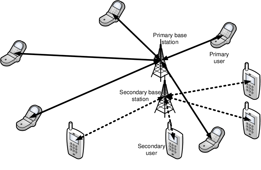
Refer to caption — Fig. 1: A cognitive radio network scenario. In the secondary network, the dotted arrows denote the channels between the secondary base station and the secondary users.

One way to realize network-based spectrum sensing is to construct a sensor network that is dedicated to sensing the radio environment in space and time [19]. The secondary base station will collect the sensing information from the sensor network and provide it to the unlicensed users, which is called “sensing as service”. There has been significant current research efforts along this direction in the context of an European project SENDORA [20], which aims at developing techniques based on sensor networks for supporting coexistence of licensed and unlicensed wireless users in a same area.

In our model, the time is divided into equal length slots. Primary users’ activities remain roughly unchanged within a single time slot. This means that it is enough for the operator to sense once at the beginning of each time slot (see Fig. 2). For readers who are interested in the optimization of the time slot length to balance sensing and data transmission, see [21].

The network has a set $\mathcal{J}=\{1,\ldots,J\}$ of orthogonal primary licensed channels. The state of each channel follows a Markovian ON/OFF process as in Fig. 3. If a channel is “ON”, then it means that the primary user is not active on the channel and the channel condition is good enough to support the transmission rate requirement of a secondary user. Here we assume that all secondary users want to achieve the same target transmission rate (e.g., that of a same type of video streaming application). If a channel is “OFF”, then either a primary user is active on this channel, or the channel condition is not good enough to achieve the secondary user’s target rate. In the time slotted system, the channel state changes from “ON” to “OFF” (“OFF” to “ON”, respectively) between adjacent time slots with a probability $p$ ( $q$ , respectively). When a channel is “ON”, it can be used by a secondary unlicensed user.

We consider an infinitely backlog case, where there are many secondary users who want to access the idle channels. Each idle channel can be used by at most one secondary user at any given time. A secondary user represents an unlicensed user communicating with the secondary base station as shown in Fig. 1. The secondary users are interested in real-time applications such as video streaming and VoIP, which require steady data rates with stringent delay constraints. The key QoS parameter is the accumulative delay, which is the total delay that a secondary user experiences after it is admitted into the system. Once a secondary user is admitted into the network, it may finish the session normally with a certain probability. However, if the user experiences an accumulative delay larger than a threshold, then its QoS significantly drops (e.g., freezing happens for video streaming) and the user will be forced to terminate.

To make the analysis tractable, we make several assumptions. First, we assume that the availabilities of all channels follow the same Markovian model. This is reasonable if the traffic types of different primary users are similar (e.g., all primary users are voice users). Second, we assume that all secondary users experience the same channel availability independent of their locations. This is reasonable when the secondary users are close-by. Third, we assume the spectrum sensing is error-free. This can be well approximated by having enough sensors performing collaborating sensing. Furthermore, we assume that all channels are homogeneous and can provide the same data rate to any single secondary user using any channel. Finally, we assume that all secondary users are homogeneous (i.e., interested in the same application such as video streaming). Each secondary user only requires one available channel to satisfy its rate requirement. Several of the above assumptions can be relaxed by increasing the state space of the MDP formulation. As we will see shortly, the admission control and channel allocation issue in this homogeneous case is already quite complicated and admits no closed-form solutions. The analysis and insights of this paper will enable us to further consider heterogeneous channels and secondary users in the future.

III Problem Formulation

We formulate the admission control and channel allocation problem as an MDP [22]. In an infinite-horizon MDP with a set of finite states $\mathcal{S}$ , the state evolves through time according to a transition probability matrix $\left\{P_{x_{k}x_{k+1}}\right\}$ , which depends on both the current state and the control decision from a set $\mathcal{U}$ . More specifically, if the network is in state $x_{k}$ in time slot $k$ and selects a decision $u(x_{k})\in\mathcal{U}(x_{k})$ , then the network obtains a revenue $g(x_{k},u(x_{k}))$ in time slot $k$ and moves to state $x_{k+1}$ in time slot $k+1$ with probability $P_{x_{k}x_{k+1}}(u(x_{k}))$ . We want to maximize the long-term time average revenue, i.e.,

\lim_{T\to\infty}E\left\{{\frac{1}{T}\sum_{k=0}^{T-1}{g(x_{k},u(x_{k}))}}\right\}.

(1)

III-A The State Space

The system state describes system information after the network performs spectrum sensing at the beginning of the time slot (see Fig. 2). It consists of two components:

•

A channel state component, $m=\boldsymbol{a}^{T}\cdot\boldsymbol{a}$ , describes the number of available channels. Here $\boldsymbol{a}=(a_{j},\forall j\in\mathcal{J})$ is the channel availability vector, where $a_{j}=1$ (or $0$ ) when channel $j$ is available (or not).
•

A user state component, $\boldsymbol{\omega_{e}}=(\omega_{e,i},\forall i\in\mathcal{D})$ , describes the numbers of secondary users with different accumulative delays. Here $\mathcal{D}=\{0,1,\ldots,D_{\max}\}$ is the set of possible delays, and $\omega_{e,i}$ denotes the number of secondary users whose accumulative delay is $i$ .

We let $\mathcal{M}$ denote the feasible set of the channel state component, and $\Omega$ denote the feasible set of the user state component. The state space is given by $\mathcal{S}=\left\{(m,\boldsymbol{\omega_{e})}|m\in\mathcal{M},\boldsymbol{\omega_{e}}\in\Omega\right\}.$

State $\theta$ is said to be accessible from state $\eta$ if and only if it is possible to reach state $\theta$ from $\eta$ , i.e., $P\{reach~\theta|start~in~\eta\}>0$ [23]. Two states that are accessible to each other are said to be able to communicate with each other. In our formulation, all the states in space $\mathcal{S}$ are accessible from state $\boldsymbol{0}$ , which is defined as a state where there is no available channel and no single admitted secondary user in the system. Since it is possible to have $m=0$ in several consecutive time slots (when primary traffic is heavy and occupies all channels), thus state $\boldsymbol{0}$ is accessible from any state in the state space $\mathcal{S}$ . Hence, all the states communicate with each other and the Markov chain is irreducible. Finally, the state space is finite, so all the states are positive recurrent [23]. This property turns out to be critical for the analysis in Section IV.

III-B The Control Space

For the state $x_{k}=\{m,\boldsymbol{\omega_{e}}\}\in\mathcal{S}$ in each time slot $k$ , the set of available control choices $\mathcal{U}(x_{k})$ depends on the relationship between the channel state and the user state. The control vector $u(x_{k})=\{u_{a},\boldsymbol{u_{e}}\}$ consists of two parts: scalar $u_{a}$ denotes the number of admitted new secondary users, and vector $\boldsymbol{u_{e}}=\{u_{e,i},\forall i\in\mathcal{D}\}$ denotes the numbers of secondary users who are allocated channels and have accumulative delays of $i\in\mathcal{D}$ at the beginning of the current time slot. Without loss of generality, we assume $0\leq u_{a}\leq J$ , i.e., we will never admit more secondary users than the total number of channels. This leads to $0\leq u_{e,0}\leq\omega_{e,0}+u_{a}$ , $0\leq u_{e,i}\leq\omega_{e,i}$ for all $i\in[1,D_{\max}]$ , and $0\leq\sum_{i=0}^{D_{\max}}{u_{e,i}}\leq m$ . Since $m\leq J$ , the cardinality of the control space $\mathcal{U}$ is $J^{D_{\max}+2}$ .

III-C The State Transition

Current state $x_{k}=\{m,\boldsymbol{\omega_{e}}\}\in\mathcal{S}$ together with the control $u(x_{k})\in\mathcal{U}(x_{k})$ determine the probability of reaching the next state $x_{k+1}=\{m^{\prime},\boldsymbol{\omega_{e}^{\prime}}\}$ .

First, the transition of channel state component from $m$ to $m^{\prime}$ depends on the underlying primary traffic. We can divide $m^{\prime}$ available channels into two groups: one group contains $m_{1}^{\prime}$ channels which are available in the (current) time slot $k$ , the other group contains $m_{2}^{\prime}$ channels which are not available in time slot $k$ . Let us define the set $\mathcal{Z}\!\!=\!\!\left\{(m_{1}^{\prime},m_{2}^{\prime})|m^{\prime}\!\!=\!\!m_{1}^{\prime}\!\!+\!\!m_{2}^{\prime},0\!\!\leq\!\!m_{1}^{\prime}\!\!\leq\!\!m,0\!\!\leq\!\!m_{2}^{\prime}\!\!\leq\!\!J\!\!-\!\!m\right\}.$ Then we can calculate the probability based on the i.i.d. ON/OFF model in Section II:

P_{mm^{\prime}}\!\!=\!\!\!\!\sum_{(m_{1}^{\prime},m_{2}^{\prime})\in\mathcal{Z}}\!\!\left\{\!\!\binom{m}{m_{1}^{\prime}}\!\!p^{m_{1}^{\prime}}(1\!\!-\!\!p)^{m\!\!-\!\!m_{1}^{\prime}}\!\!\binom{J\!\!-\!\!m}{m_{2}^{\prime}}\!\!(1\!\!-\!\!q)^{m_{2}^{\prime}}q^{J\!\!-\!\!m\!\!-\!\!m_{2}^{\prime}}\right\}.

(2)

Thus the channel transition function is $f_{s}(m)=m^{\prime}$ with probability $P_{mm^{\prime}}$ for all $m^{\prime}\in{\mathcal{M}}$ .

Let us define $\boldsymbol{\omega_{c}}=\{\omega_{c,i},\forall i\in\mathcal{D}\}$ as the number of secondary users who normally complete their connections (not due to delay violation) in time slot $k$ . For example, a user may terminate a video streaming session after the movie finishes, or terminate a VoIP session when the conversation is over. If we assume that all users have the same completion probability $P_{f}$ per slot when they are actively served, then the event of having $\rho$ out of $\tau$ users completing their connections (denoted as $f_{c}(\tau)=\rho$ ) happens with probability $\binom{\tau}{\rho}{P_{f}^{\rho}(1-P_{f})^{\tau-\rho}}$ .

Finally, define $\omega_{q}$ as the number of secondary users who are forced to terminate their connections during time slot $k$ . The state transition can be written as

\left\{\begin{split}&m^{\prime}=f_{s}(m),\\ &\omega_{c,i}=f_{c}(u_{e,i}),\forall i\in\mathcal{D},\\ &\omega_{q}=\omega_{e,D_{\max}}-u_{e,D_{\max}},\\ &\omega_{e,0}^{\prime}=u_{e,0}-\omega_{c,0},\\ &\omega_{e,1}^{\prime}\!=\!u_{e,1}+(\omega_{e,0}+u_{a}-u_{e,0})-\omega_{c,1},\\ &\omega_{e,i}^{\prime}\!=\!u_{e,i}\!+\!(\omega_{e,i-1}-u_{e,i-1})\!-\!\omega_{c,i},\forall i\in[2,D_{\max}].\end{split}\right.

(3)

Let us take a network with $J=10$ and $D_{max}=2$ as a numerical example. In a particular time slot, assume that there are $m=7$ channels available and a total of $6$ secondary users admitted in the system: $1$ user with zero accumulative delay, $3$ users with $1$ time slot of accumulative delay, and $2$ users with $2$ time slots of accumulative delay. Then the state vector is $\{m,\boldsymbol{\omega_{e}}\}=\{7,(1,3,2)\}$ . Assume the control decision is to admit $2$ new users and to allocate available channels to the users except one of the new users, i.e., $u=\{u_{a},\boldsymbol{u_{e}}\}=\{2,(2,3,2)\}$ . Thus if there is no user completing a connection in the current time slot and $m^{\prime}=4$ available channels in the next time slot, the system state becomes $\{m^{\prime},\boldsymbol{\omega_{e}^{\prime}}\}=\{4,(2,4,2)\}$ .

III-D The Objective Function

Our system optimization objective is to choose the optimal control decision for each possible state to maximize the expected average revenue per time slot (also called stage), i.e.,

\max{\lim_{T\to\infty}E\left\{{\frac{1}{T}\sum_{k=0}^{T-1}{g(x_{k},u(x_{k}))}}\right\}}.

(4)

Here the revenue function is computed at the end of each time slot $k$ as follows:

g(x_{k},u(x_{k}))\!\!=\!\!R_{c}\!\!\sum_{i=0}^{D_{\max}}{\omega_{c,i}(k)}\!\!+\!\!R_{t}\!\!\sum_{i=0}^{D_{\max}}{\omega_{e,i}}(k)\!\!-\!\!C_{q}\omega_{q}(k),

(5)

where $R_{c}\geq 0$ is the reward of completing the connection of a secondary user normally (without violating the maximum delay constraints), $R_{t}\geq 0$ is the reward of maintaining the connection of a secondary user, and $C_{q}\geq 0$ is the penalty of forcing to terminate a connection. By choosing different values of $R_{c}$ , $R_{t}$ , and $C_{q}$ , a network designer can achieve different objective functions. In this paper, we assume that the values of $R_{c}$ , $R_{t}$ , and $C_{q}$ are given parameters.

IV Analysis of the MDP Problem

We define a sequence of control actions as a policy, ${\boldsymbol{\mu}}=\left\{u(x_{0}),u(x_{1}),\cdots\right\}$ , where $u(x_{k})\in\mathcal{U}(x_{k})$ for all $k$ . A policy is stationary if the choice of decision only depends on the state and is independent of the time. Let

V_{\boldsymbol{\mu}}(\theta)=\lim_{T\to\infty}E\left\{\frac{1}{T}\sum_{k=0}^{T-1}g(x_{k},u(x_{k}))|x_{0}=\theta\right\}

be the expected revenue in state $\theta$ under policy $\boldsymbol{\mu}$ . Our objective is to find the best policy $\boldsymbol{\mu^{\ast}}$ to optimize the average revenue per stage starting from an initial state $\theta$ .

Section III-A shows that any state can be visited from any other state within finite stages under a stationary policy.¹¹ 1 A policy is stationary if the choice of decision only depends on the state and is independent of the time. Moreover, since the revenue $g(x_{k},u(x_{k}))<\infty$ for all $x_{k}$ and $u$ , we have

\lim_{T\to\infty}\frac{1}{T}E\left\{\sum_{k=0}^{K}g(x_{k},u(x_{k}))\right\}=0

(6)

for any finite $K$ . Therefore, we have the following proposition in our prior preliminary results [1].

Proposition 1

For any stationary policy, the average revenue per stage is independent of the initial state.

Next we give the following detailed proof of the proposition.

Proof:

Since the revenue $g(x_{k},u(x_{k}))<\infty$ for all $x_{k}$ and $u$ , we have

\lim_{T\to\infty}\frac{1}{T}E\left\{\sum_{k=0}^{K}g(x_{k},u(x_{k}))\right\}=0

(7)

for any finite value of $K$ . Consider a stationary policy $\boldsymbol{\mu}$ whose control decision only depends on the state of the system. According to the MDP formulation, all the states are positive recurrent. So starting in state $\theta$ , the process will visit state $\eta$ infinitely often; and the expected time that the process visits state $\eta$ from state $\theta$ is finite [23]. Thus, any state in the state space can be visited from any other state within enough stages (finite) under the stationary policy. Therefore, we assume, under the policy $\boldsymbol{\mu}$ , the state $\eta\in\mathcal{S}$ is visited from the state $\theta\in\mathcal{S}$ . Let $K_{\theta\eta}(\boldsymbol{\mu})$ be the number of time slots that the system first passes state $\eta$ from state $\theta$ under policy $\boldsymbol{\mu}$ , then the average revenue per stage corresponding to initial condition $x_{0}=\theta$ can be expressed as

\begin{split}V_{\boldsymbol{\mu}}(\theta)=&\lim_{T\to\infty}\frac{1}{T}E\left\{\sum_{k=0}^{K_{\theta\eta}(\boldsymbol{\mu})-1}g(x_{k},u(x_{k}))\right\}\\ &+\lim_{T\to\infty}\frac{1}{T}E\left\{\sum_{k=K_{\theta\eta}(\boldsymbol{\mu})}^{T-1}g(x_{k},u(x_{k}))\right\}.\end{split}

(8)

The first term in (8) is zero according to (7), while the second limit is equal to $V_{\boldsymbol{\mu}}(\eta)$ . So with $E\{K_{\theta\eta}(\boldsymbol{\mu})\}<\infty$ ,

V_{\boldsymbol{\mu}}(\theta)=V_{\boldsymbol{\mu}}(\eta)=V_{\boldsymbol{\mu}},

(9)

for any two states $\theta$ and $\eta$ . ∎

As shown in Proposition 1, the average revenue per stage under any stationary policy is independent of the initial state, and the average revenue maximization problem could be transformed into the stochastic shortest path problem. More specifically, we pick a state $n$ as the start state of the stochastic shortest path problem, and define an artificial termination state $t$ from the state $n$ . The transition probability from an arbitrary state $\theta$ to the termination state $t$ satisfies $P_{\theta t}(\boldsymbol{\mu})=P_{\theta n}(\boldsymbol{\mu})$ , as show in Fig. 4.

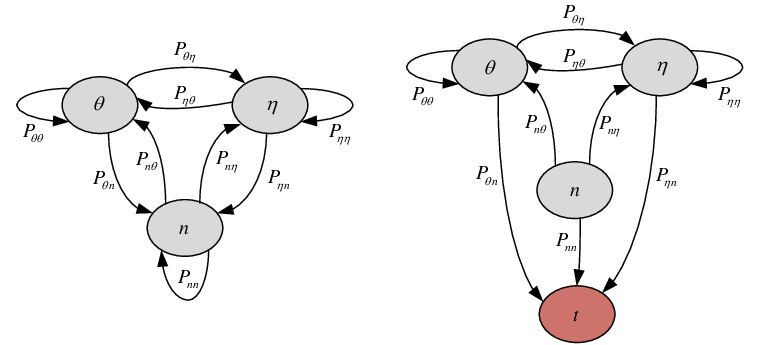
In the stochastic shortest path problem, we define $-\hat{g}(n,\boldsymbol{\mu})$ as the expected stage cost incurred at state $n$ under policy $\boldsymbol{\mu}$ . Let $A^{\ast}$ be the optimal average revenue per stage starting from the state $n$ to the terminal state $t$ , and let $A^{\ast}-\hat{g}(n,\boldsymbol{\mu})$ be the normalized expected stage cost. Then the normalized expected terminal cost from the state $x_{0}=n$ under the policy $\boldsymbol{\mu}$ , $h^{\boldsymbol{\mu}}(n)=\lim_{N\to\infty}{E\left\{\sum_{k=0}^{N-1}\left\{A^{\ast}-g(x_{k},u(x_{k}))\right\}\right\}}$ , is zero when the policy $\boldsymbol{\mu}$ is optimal. The cost minimization in the stochastic shortest path problem is equivalent to the original average revenue per stage maximization problem. Let $h^{\ast}(\theta)$ denote the optimal cost of the stochastic shortest path starting at state $\theta\in\mathcal{S}$ , then we get the corresponding Bellman’s equation as follows [22]:

h^{\boldsymbol{\mu}}(\theta)\!\!=\!\!\min_{\boldsymbol{\mu}}\left\{A^{\ast}\!\!-\!\!\hat{g}(\theta,\boldsymbol{\mu})\!\!+\!\!\sum_{\eta\in\mathcal{S}}p_{\theta\eta}(\boldsymbol{\mu})h^{\boldsymbol{\mu}}(\eta)\right\},~\theta\in\mathcal{S}.

(10)

If $\boldsymbol{\boldsymbol{\mu}^{\ast}}$ is a stationary policy that maximizes the cycle revenue, we have the following equations:

h^{\ast}(\theta)=A^{\ast}-\hat{g}(\theta,\boldsymbol{\mu}^{\ast})+\sum_{\eta\in\mathcal{S}}p_{\theta\eta}(\boldsymbol{\mu}^{\ast})h^{\ast}(\eta),~\theta\in\mathcal{S}.

(11)

The Bellman’s equation is an iterative way to solve MDP problems. Next we show that solving the Bellman’s equation (12) in the stochastic shortest path problem leads to the optimal solution.

Proposition 2

For the stochastic shortest path problem, given any initial values of terminal costs $h_{0}(\theta)$ for all states $\theta\in\mathcal{S}$ , the sequence $\{h_{l}(\theta),l=1,2,\ldots\}$ generated by the iteration

h_{l+1}(\theta)\!\!=\!\!\min_{\boldsymbol{\mu}}{\left\{A^{\ast}\!\!-\!\!\hat{g}(\theta,\boldsymbol{\mu})\!\!+\!\!\sum_{\eta\in\mathcal{S}}P_{\theta\eta}(\boldsymbol{\mu})h_{l}(\eta)\right\},{\theta\in\mathcal{S},}}

(12)

converges to the optimal terminal cost $h^{\ast}(\theta)$ for each state $\theta$ .

Proof:

For an arbitrary state $\theta$ and an admissible policy $\boldsymbol{\mu}$ , there exists an integer $\gamma$ satisfying $P\{x_{\gamma}\neq t|x_{0}=\theta,\boldsymbol{\mu}\}<1$ [24]. Let $\rho=\max_{(\theta,\boldsymbol{\mu})}{P\{x_{\gamma}\neq t|x_{0}=\theta,\boldsymbol{\mu}\}}$ , then $\rho<1$ and $P\left\{x_{2\gamma}\neq t|x_{0}=\theta,\boldsymbol{\mu}\right\}=P\{x_{2\gamma}\neq t|x_{\gamma}\neq t,x_{0}=\theta,\boldsymbol{\mu}\}\cdot P\{x_{\gamma}\neq t|x_{0}=\theta,\boldsymbol{\mu}\}\leq\rho^{2}.$ Therefore, we get $P\{x_{\phi\gamma}\neq t|x_{0}=\theta,\boldsymbol{\mu}\}\leq\rho^{\phi}.$

We break down the cost $h^{\boldsymbol{\mu}}(x_{0})$ into the portions incurred over the first $K\gamma$ time slots ( $K$ is a positive integer) and over the remaining time slots, i.e.,

\begin{split}h^{\boldsymbol{\mu}}(x_{0})=&\lim_{N\to\infty}{E\left\{\sum_{k=0}^{N-1}\left\{A^{\ast}-g(x_{k},u(x_{k}))\right\}\right\}}\\ =&E\left\{\sum_{k=0}^{K\gamma-1}\left\{A^{\ast}-g(x_{k},u(x_{k}))\right\}\right\}\\ &+\lim_{N\to\infty}{E\left\{\sum_{k=K\gamma}^{N-1}\left\{A^{\ast}-g(x_{k},u(x_{k}))\right\}\right\}}.\end{split}

(13)

Define $\Gamma=\gamma\max_{(\theta,\boldsymbol{\mu})}{\left|A^{\ast}-\hat{g}(\theta,\boldsymbol{\mu})\right|}$ , which denotes the upper bound on the cost of an $\gamma$ -slot cycle when termination does not occur during the cycle. Then, the expected cost during the $K$ -th $\gamma$ -slot cycle (time slots $K\gamma$ to $(K+1)\gamma-1$ ) is upper bounded by $\rho^{K}\Gamma$ , so that

\begin{split}&E\left\{\left|h^{\boldsymbol{\mu}}(x_{0})-\sum_{k=0}^{K\gamma-1}\{A^{\ast}-g(x_{k},u(x_{k}))\}\right|\right\}\\ &=\left|\lim_{N\to\infty}{E\left\{\sum_{k=K\gamma}^{N-1}\{A^{\ast}-g(x_{k},u(x_{k}))\}\right\}}\right|\\ &\leq\Gamma\sum_{\phi=K}^{\infty}{\rho^{\phi}}=\frac{\rho^{K}\Gamma}{1-\rho}.\end{split}

(14)

Let $h_{0}(x_{0})$ be a terminal cost function as defined in the proposition, and then its expected value under $\boldsymbol{\mu}$ after $K\gamma$ time slots is bounded by

\begin{split}\left|E\{h_{0}(x_{K\gamma})\}\right|&\!\!=\!\!\left|\sum_{\theta\in\mathcal{S}}{P(x_{K\gamma}=\theta|x_{0},\boldsymbol{\mu})h_{0}(\theta)}\right|\\ &\!\!\leq\!\!\left(\sum_{\theta\in\mathcal{S}}{P(x_{K\gamma}=\theta|x_{0},\boldsymbol{\mu})}\right)\!\!\max_{\theta\in\mathcal{S}}{|h_{0}(\theta)|}.\end{split}

(15)

Since the probability that $x_{K\gamma}\neq t$ is less than or equal to $\rho^{K}$ for any policy, we have $\left|E\{h_{0}(x_{K\gamma})\}\right|\leq\rho^{K}\max_{\theta\in\mathcal{S}}{|h_{0}(\theta)|}$ . Therefore, we can get

\begin{split}&-\rho^{K}\max_{\theta\in\mathcal{S}}{|h_{0}(\theta)|}+h^{\boldsymbol{\mu}}(x_{0})-\frac{\rho^{K}\Gamma}{1-\rho}\\ &\leq E\left\{h_{0}(x_{K\gamma})+\sum_{k=0}^{K\gamma-1}\{A^{\ast}-g(x_{k},u(x_{k}))\}\right\}\\ &\leq\rho^{K}\max_{\theta\in\mathcal{S}}{|h_{0}(\theta)|}+h^{\boldsymbol{\mu}}(x_{0})+\frac{\rho^{K}\Gamma}{1-\rho}.\end{split}

(16)

The expected value in the middle term of the above inequalities is the $K\gamma$ -slot cost of policy $\boldsymbol{\mu}$ starting from state $x_{0}$ with a terminal cost $h_{0}(x_{K\gamma})$ . The minimum of this cost over all $\boldsymbol{\mu}$ is equal to the value $h_{K\gamma}(x_{0})$ , which is generated by the dynamic programming recursion (12) after $K\gamma$ iterations. Thus, by taking the minimum over $\boldsymbol{\mu}$ in (16), we obtain for all $x_{0}$ and $K$ ,

\begin{split}-\rho^{K}\max_{\theta\in\mathcal{S}}{|h_{0}(\theta)|}+h^{\ast}(x_{0})-\frac{\rho^{K}\Gamma}{1-\rho}\leq h_{K\gamma}(x_{0})&\\ \leq\rho^{K}\max_{\theta\in\mathcal{S}}{|h_{0}(\theta)|}+h^{\ast}(x_{0})+\frac{\rho^{K}\Gamma}{1-\rho}.&\end{split}

(17)

And by taking the limit when $K\to\infty$ , the terms involving $\rho^{K}$ will go to zero, and we obtain $\lim_{K\to\infty}{h_{K\gamma}(x_{0})}=h^{\ast}(x_{0})$ for all $x_{0}$ . In addition, since $\left|h_{K\gamma+q}(x_{0})-h_{K\gamma}(x_{0})\right|\leq\rho^{K}\Gamma,\;q=1,2,\cdots,\gamma-1$ , we have $\lim_{K\to\infty}{h_{K\gamma+q}(x_{0})}=\lim_{K\to\infty}{h_{K\gamma}(x_{0})}=h^{\ast}(x_{0})$ for all $q=1,\cdots,\gamma-1$ . ∎

Proposition 2 shows that solving the Bellman’s equation leads to the optimal average revenue $A^{\ast}$ and the optimal differential cost $h^{\ast}$ . The Bellman’s equation can often be solved using value iteration or policy iteration algorithms; details can be found in [24] and [25]. Once having $A^{\ast}$ and $h^{\ast}$ , we can compute the optimal control decision $u^{\ast}(\theta)$ that minimizes the immediate differential cost of the current stage plus the remaining expected differential cost for state $\theta$ , i.e.,

u^{\ast}(\theta)\!=\!\arg{\min_{\boldsymbol{\mu}}{\left\{A^{\ast}\!-\!\hat{g}(\theta,\boldsymbol{\mu})\!+\!\sum_{\eta\in\mathcal{S}}{p_{\theta\eta}(\boldsymbol{\mu})h^{\ast}(\eta)}\right\}}}.

(18)

V Suboptimal Control and Dynamic Programming

Solving the Bellman’s equation does not lead to a closed-form optimal control policy, and the iterative computation is time-consuming for our problem with a large state space. To resolve this issue, a broad class of suboptimal control methods referred as approximate dynamic programming (ADP) have been proposed in [22]. Next we first propose a simple heuristic control policy in Section V-A. Then in Section V-B, we will improve the performance of the heuristic algorithm by using the idea of rollout algorithm (which is a class of ADP algorithms). It is known that the suboptimal policy based on the rollout algorithm is identical to the policy obtained by a single policy improvement step of the classical policy iteration method [24, 25].

V-A Heuristic Control Policy

Several observations can help us with the suboptimal algorithm design. First, the channel state transitions are determined by the underlying primary traffic and are not affected by any control policy. Second, all secondary users experience the same channel availability independent of their locations, and all channels are homogenous and provide the same data rates. This means that we are interested in how many users to admit rather than who to admit, and we only care how many channels are available instead of which are available. This motivates us to first consider admission control and channel allocation separately.

For the admission control, we first consider a simple threshold-based strategy, where a new user will be admitted if and only if the total number of admitted users is smaller than the threshold. Given a fixed admission control threshold $T_{h}$ , there are many ways of performing the channel allocation. To resolve this issue, we propose the largest-delay-first strategy, which allocates available channels to admitted users with the largest accumulated delay first.

Proposition 3

The largest-delay-first channel allocation policy is optimal under any fixed threshold-based admission control policy.

Proof:

Under a threshold-based admission control policy, the number of admitted users in the system is constant in any time slot. The objective function in (4) is equal to the maximization problem $\max{E\left\{g(x,u(x))\right\}}$ due to ergodicity of the instant revenue $g(x_{k},u(x_{k}))$ . Let $\Omega_{c}=E\left\{\sum_{i=0}^{D_{max}}{\omega_{c,i}}\right\}$ be the expected number of normally completed users at the end of each time slot, $\Omega_{e}=E\left\{\sum_{i=0}^{D_{max}}{\omega_{e,i}}\right\}$ be the expected number of users in the network at the end of each time slot, and $\Omega_{q}=E\left\{\omega_{q}\right\}$ be the expected number of forcefully terminated users at the end of each time slot. Then

\max{E\left\{g(x,u(x))\right\}}=\max{\left\{R_{c}\Omega_{c}+R_{t}\Omega_{e}-C_{q}\Omega_{q}\right\}}.

(19)

Under the threshold-based admission control policy, $\Omega_{e}=\sum_{i=0}^{D_{max}}{\omega_{e,i}}$ in all time slot $k$ and equals to the threshold.

In the largest-delay-first policy, let $L_{c}$ be the expected length of a normally completed session, $D_{c}$ the expected delay of a normally completed session, and $L_{q}$ the expected length of a forcefully terminated session. Now let us consider an arbitrary channel allocation policy as the benchmark, and we use the superscript ${(g)}$ to denote all parameters corresponding to this particular channel allocation policy, i.e., $\Omega_{c}^{(g)}$ , $\Omega_{e}^{(g)}$ , $\Omega_{q}^{(g)}$ , $L_{c}^{(g)}$ , $D_{c}^{(g)}$ , and $L_{q}^{(g)}$ . We will show that the largest-delay-first policy is no worse than this benchmark policy, which will prove the proposition.

Because all actively served users have the same completion probability $P_{f}$ independent of the channel allocation decisions, we can show that $\Omega_{c}=\Omega_{c}^{(g)},$ $\Omega_{e}=\Omega_{e}^{(g)}$ , and $L_{c}=L_{c}^{(g)}$ . Since the largest-delay-first policy always allocates available channels to the secondary users with the largest delay, we have $D_{c}\geq D_{c}^{(g)}.$

Here comes the critical proof step. We consider $\Omega_{e}$ virtual channels, one for each user in the network. If the secondary user is allocated an available physical channel, then its virtual channel is “idle” in that time slot; otherwise its virtual channel is “busy” and causes a delay. In the long run (when $T\to\infty$ ), we have the following:

\begin{split}\Omega_{e}\cdot T&=\Omega_{c}T(L_{c}+D_{c})+\Omega_{q}T(L_{q}+D_{max})\\ &=\Omega_{c}^{(g)}T(L_{c}^{(g)}+D_{c}^{(g)})+\Omega_{q}^{(g)}T(L_{q}^{(g)}+D_{max}).\end{split}

(20)

Based on the relationships we just derived in the previous paragraph, we have

\Omega_{q}(L_{q}+D_{max})\leq\Omega_{q}^{(g)}(L_{q}^{(g)}+D_{max}).

(21)

Since the number of available channels is the same under the two channel allocation policies in any time slot , we have

\Omega_{c}TL_{c}+\Omega_{q}TL_{q}=\Omega_{c}^{(g)}TL_{c}^{(g)}+\Omega_{q}^{(g)}TL_{q}^{(g)}.

(22)

Since $\Omega_{c}=\Omega_{c}^{(g)}$ and $L_{c}=L_{c}^{(g)}$ , (22) implies that $\Omega_{q}L_{q}=\Omega_{q}^{(g)}L_{q}^{(g)}$ . Together with inequality (21), we have $\Omega_{q}\leq\Omega_{q}^{(g)}.$

Because $\Omega_{c}=\Omega_{c}^{(g)},$ $\Omega_{e}=\Omega_{e}^{(g)}$ , and $\Omega_{q}\leq\Omega_{q}^{(g)}$ , we have $R_{c}\Omega_{c}+R_{t}\Omega_{e}-C_{q}\Omega_{q}\geq R_{c}\Omega_{c}^{(g)}+R_{t}\Omega_{e}^{(g)}-C_{q}\Omega_{q}^{(g)},$ i.e., $\max{E\left\{g(x_{k},u(x_{k}))\right\}}\geq\max{E\left\{g^{(g)}(x_{k},u(x_{k}))\right\}}.$ This shows that our proposed largest-delay-first channel allocation policy is no worse than any channel allocation algorithm, and thus is optimal with a threshold-based admission control. ∎

For performance comparison, we further define two benchmark channel allocation strategies.

•

Strategy 1: allocate the available channels to the admitted users with the smallest accumulated delays. If there is a tie, break it randomly.
•

Strategy 2: allocate the available channels to the admitted users randomly.

In Fig. 5 and Fig. 6, we compare the proposed channel allocation policy and the two benchmark policies with different total number of channels. All three policies follow the same threshold-based admission control policies. From these figures, we observe that the proposed largest-delay-first policy is no worse than the other two under all choices of parameters.

V-B Rollout Control Policy

The heuristic algorithm proposed in Section V-A can be further improved by the rollout algorithm. The general background of the rollout algorithm is in Appendix -A. In this subsection, based on the analysis of the heuristic control policy, we propose a simplified rollout algorithm (rollout control policy) to further improve the performance.

Consider two different user states $\boldsymbol{\omega_{e}^{(1)}}$ and $\boldsymbol{\omega_{e}^{(2)}}$ that have the same number of secondary users. If it is possible for transit from state $\boldsymbol{\omega_{e}^{(1)}}$ to state $\boldsymbol{\omega_{e}^{(2)}}$ under a particular channel condition without admitting any new user, then obviously the total time delay of $\boldsymbol{\omega_{e}^{(1)}}$ summed over all users must be less than that of $\boldsymbol{\omega_{e}^{(2)}}$ (as each user either has the same delay or a larger delay during the transition). We give the following definitions:

Definition 1 (User State Comparison)

Consider two different user states $\boldsymbol{\omega_{e}^{(1)}}$ and $\boldsymbol{\omega_{e}^{(2)}}$ that have the same number of secondary users. If it is possible to transit from state $\boldsymbol{\omega_{e}^{(1)}}$ to state $\boldsymbol{\omega_{e}^{(2)}}$ under a particular channel condition without admitting any new user, then $\boldsymbol{\omega_{e}^{(1)}}$ is better than $\boldsymbol{\omega_{e}^{(2)}}$ , denoted $\boldsymbol{\omega_{e}^{(1)}}\gtrdot\boldsymbol{\omega_{e}^{(2)}}$ .

Definition 2 (Quality of Channel State)

Consider a user state $\boldsymbol{\omega_{e}^{(1)}}$ and a channel state $m$ . The channel state $m$ is $\boldsymbol{B}$ (Bad) for the user state $\boldsymbol{\omega_{e}^{(1)}}$ if and only if $m$ is less than the total number of users in $\boldsymbol{\omega_{e}^{(1)}}$ . Otherwise, the channel state $m$ is $\boldsymbol{G}$ (Good) for the user state $\boldsymbol{\omega_{e}^{(1)}}$ .

Now consider a heuristic control policy with the admission control threshold $N_{th}$ and largest-delay-first channel allocation mechanism. Under this policy, we can divide the infinite-horizon process into infinite number of segments separated by the time slots in which there is at least one user leaving the system (normal completion or forced termination). Then we can define a new average revenue $\bar{g}(N_{th},\theta)$ and its expectation $\bar{G}(N_{th},\theta)$ ) over each segment. Due to the threshold-based admission control, we will only admit new users in the first slot of a segment.

Definition 3 (Average Revenue and Expected Average Revenue)

If the network state is $\theta$ at the beginning of time slot $k$ , and at least one user leaves the system for the first time (normal completion or forced termination) in time slot $k+\delta$ , we define the average revenue over the period $[k,k+\delta]$ as

\bar{g}(N_{th},\theta)\!=\!\frac{n_{c}(N_{th},\theta)}{\delta+1}R_{c}\!-\!\frac{n_{d}(N_{th},\theta)}{\delta+1}C_{q}\!+\!N_{th}R_{t},

(23)

where $n_{c}(N_{th},\theta)$ is number of users completing connections normally in time slot $k+\delta$ , and $n_{d}(N_{th},\theta)$ is number of users being forced to terminate in time slot $k+\delta$ . The expected average revenue is denoted as

\begin{split}\bar{G}(N_{th},\theta)&=E\{\bar{g}(N_{th},\theta)\}\\ &=\!N_{c}(N_{th},\theta)R_{c}\!-\!N_{d}(N_{th},\theta)C_{q}\!+\!N_{th}R_{t},\end{split}

(24)

where $N_{c}(N_{th},\theta)=E\left\{\frac{n_{c}(N_{th},\theta)}{\delta+1}\right\}$ and $N_{d}(N_{th},\theta)=E\left\{\frac{n_{d}(N_{th},\theta)}{\delta+1}\right\}.$

The expected revenue in Definition 3 is different from the instant revenue in (5). The expected revenue is defined under a very special case, where no new users are admitted except in the first time slot and no users leave the network except in the last time slot of the interval. The instant revenue defined in (5) is the revenue for a generic time slot. Furthermore, $\bar{G}(N_{th},\theta)$ represents the expected average revenue per time slot when maintaining a fixed number of users until someone leaves. Although the precise value of $\bar{G}(N_{th},\theta)$ is hard to compute explicitly, we have the following result as a corollary of Proposition 3.

Proposition 4

Given any fixed $N_{th}$ and $\theta$ , the largest-delay-first channel allocation policy achieves the maximum $\bar{G}(N_{th},\theta)$ .

Based on Proposition 4, we will still use the largest-delay-first strategy channel allocation. The key remaining issue is how to improve the admission control policy. Next we characterize the properties of the largest-delay-first channel allocation policy (the expected average revenue $\bar{G}(N_{th},\theta)$ in the heuristic control policy) in several lemmas, which enable us to design a better heuristic algorithm for the admission control part.

According to the lemmas given in Appendix -B, we can characterize $\bar{G}(N_{th},\theta)$ as follows.

Proposition 5

$\bar{G}(N_{th},\theta)$ is a concave function of $N_{th}$ .

Proof:

The second order derivative of $\bar{G}(N_{th},\theta)$ in terms of $N_{th}$ is

\bar{G}^{\prime\prime}(N_{th},\theta)=N_{c}^{\prime\prime}(N_{th},\theta)R_{c}-N_{d}^{\prime\prime}(N_{th},\theta)C_{q},

(25)

where $N_{c}^{\prime\prime}(N_{th},\theta)<0$ and $N_{d}^{\prime\prime}(N_{th},\theta)>0$ based on Lemma 1 and Lemma 2 in Appendix -B. Thus we have $\bar{G}^{\prime\prime}(N_{th},\theta)<0$ , i.e., $\bar{G}(N_{th},\theta)$ is a concave function of $N_{th}$ . ∎

Figure 7 plots $\bar{G}(N_{th},\theta)$ versus $N_{th}$ with fixed $\theta=\left\{m,[0,0,0,0,0,0]\right\}$ and different values of $R_{c}$ and $C_{q}$ .

Now we are ready to discuss the heuristic admission control policy. Given a state $\theta=(m,\boldsymbol{\omega_{e}})$ , the admission control decision can be either maintaining or searching, depending on the relationship between the channel state component $m$ and user state component $\boldsymbol{\omega_{e}}$ . More precisely, if $m$ is $\boldsymbol{B}$ (Bad) for $\boldsymbol{\omega_{e}}$ , the network coordinator will maintain the current user population and do not admit any new user (i.e., maintaining). This is because the network resource is not enough to support the current users, and admitting new users will make the situation worse. If $m$ is $\boldsymbol{G}$ (Good) for $\boldsymbol{\omega_{e}}$ , the network coordinator first searches for the value of $N_{th}^{\ast}$ that achieves $\max_{N_{th}}\bar{G}(N_{th},\theta)$ (i.e., searching), and then admits the number of users equal to the difference between $N_{th}^{\ast}$ and the current users in the network. Proposition 5 shows that $\bar{G}(N_{th},\theta)$ has a unique maximizer $N_{th}^{\ast}$ (with a fixed state $\theta$ ), and implies a simple stopping rule for the numerical search. If we have $\bar{G}(N_{th}^{\prime}-1,\theta)\leq\bar{G}(N_{th}^{\prime},\theta)$ and $\bar{G}(N_{th}^{\prime},\theta)\geq\bar{G}(N_{th}^{\prime}+1,\theta)$ , then $N_{th}^{\ast}=N_{th}^{\prime}$ .

The heuristic admission control introduced above is a rollout control policy based on the theory in Appendix -A. More specifically, the value of $\max_{N_{th}}\bar{G}(N_{th},\theta)$ computed in the searching step is the cost-to-go starting from a state $\theta$ . As Proposition 5 shows that this is a concave maximization problem, we can use several well-known numerical methods to achieve this. One possibility is the gradient decent method, which has a linear convergence rate as shown in [26]. More precisely, the maximum number of convergence of the gradient decent method is proportional to $\log{(\bar{G}(N_{th}^{initial},\theta)-\bar{G}(N_{th}^{optimal},\theta))}/{\epsilon}$ , where $\epsilon$ is the stopping criterion. Since the precise value of $\bar{G}(N_{th},\theta)$ is hard to compute with a low complexity, we will use an approximation $\tilde{G}(N_{th},\theta)$ instead in the searching step. In this paper, we use an on-line computation (simulation) to get $\tilde{G}(N_{th},\theta)$ . Mover specifically, for each choice of $(N_{th},\theta)$ , we can obtain the value of $\bar{g}((N_{th},\theta))$ as in (23) for each particular simulation, and take the average over many simulations to obtain an approximation $\tilde{G}(N_{th},\theta)$ . The memory requirements are proportional to the expected length of the segments separated by the time slots in which there is at least one user leaving the system (normal completion or forced termination)

V-C Revenue Boundary

In this subsection, we will compare the performance of two heuristic policies that we have proposed. Before that, we will establish an upper-bound of the revenue achievable under any control policy (heuristic or optimal). We call the bound the revenue boundary.

We first prove the following property of the expected average revenue $\bar{G}(N_{th},\theta)$ .

Proposition 6

For a fixed number of users $N_{th}$ , if there are two states $\theta_{1}=\left\{m,\boldsymbol{\omega_{e}^{(1)}}\right\}$ and $\theta_{2}=\left\{m,\boldsymbol{\omega_{e}^{(2)}}\right\}$ such that $\boldsymbol{\omega_{e}^{(1)}}\gtrdot\boldsymbol{\omega_{e}^{(2)}}$ , we have $\bar{G}(N_{th},\theta_{1})>\bar{G}(N_{th},\theta_{2})$ .

Proof:

According to Lemma 3 in Appendix -B, we have $N_{c}(N_{th},\theta_{1})>N_{c}(N_{th},\theta_{2})$ and $N_{d}(N_{th},\theta_{1})<N_{d}(N_{th},\theta_{2})$ . By substituting them into (24), we get $\bar{G}(N_{th},\theta_{1})>\bar{G}(N_{th},\theta_{2})$ . ∎

Then we can characterize the revenue boundary.

Proposition 7

Consider a network state $\bar{\theta}=\left\{m,[0,0,0,\cdots]\right\}$ , where there are $m$ available channels. The maximum expected revenue per time slot achieved by any policy, denoted by $G_{max}$ , satisfies $G_{max}<\max_{m,N_{th}}\left\{\bar{G}(N_{th},\bar{\theta})\right\},$ where $N_{th}$ is an admission control threshold.

Proof:

Assume $\hat{\theta}=\left\{m,\boldsymbol{\omega_{e}^{\theta}}\right\}$ and $\eta=\left\{m,\boldsymbol{\omega_{e}^{\eta}}\right\}$ are two network states with $m$ available channels and $N_{th}$ users, where $\boldsymbol{\omega_{e}^{\theta}}=[N_{th},0,0,\cdots]$ . If $\boldsymbol{\omega_{e}^{\eta}}\neq\boldsymbol{\omega_{e}^{\theta}}$ , we have $\boldsymbol{\omega_{e}^{\theta}}\gtrdot\boldsymbol{\omega_{e}^{\eta}}$ . From Proposition 6, we get $\bar{G}(N_{th},\hat{\theta})>\bar{G}(N_{th},\eta)$ . In addition, after the control decision in the first time slot, $N_{th}$ new secondary users are admitted in the case of $\overline{\theta}$ (since there are originally no users in the system), and no new secondary user is admitted in the case of $\hat{\theta}$ (since there are already $N_{th}$ users with zero accumulative delay in the system). Thus, after the first time slot, we achieve the same state in both cases. In the following time slots, the expected changes of the two cases are thus the same. Therefore, according to the definition of $\overline{G}$ in Definition 3, we have $\bar{G}(N_{th},\bar{\theta})=\bar{G}(N_{th},\hat{\theta})$ . Therefore, the cost-to-go we compute in the search step is never larger than $\max_{m,N_{th}}\left\{\bar{G}(N_{th},\bar{\theta})\right\}$ . As the optimal policy can be viewed as a special case of the rollout policy by using the optimal policy as the base policy, it follows that the expected revenue per time slot of any policy (including the optimal one) is less than $\max_{m,N_{th}}\left\{\bar{G}(N_{th},\bar{\theta})\right\}$ . ∎

In Section II, we have assumed perfect spectrum sensing. Under this assumption, the control policy of the throughput maximization problem studied in [4, 5] can be simplified into admitting secondary users to make full use of the available channels in each time slot, which we call greedy admission control in this paper. Such greedy admission control policy will admit new users whenever possible such that the total active users in a time slot equals to the number of available channels. Comparing with our proposed policy, this greedy policy is more aggressive and does not consider channel availabilities in the future, and thus will lead to a larger number of forced dropped users. We have plotted the expected revenue of the greedy admission control in Fig. 8, with the comparison with our proposed admission control and the revenue boundary. We can see that even the performance of our proposed heuristic control policy is better than that of the greedy control policy. The heuristic control policy (with the threshold-based admission control) is simple but effective, while the rollout algorithm achieves a slightly better performance but with a much higher computational complexity. The actual performance gap between the proposed algorithms and the optimal policy could be even smaller, as the revenue boundary in Proposition 7 may not be very tight.

VI Conclusions

Supporting QoS over cognitive radio networks is very challenging, mainly due to the uncertainty of available communication resources. As one further step towards understanding this under-explored yet practically important research area, we considered supporting delay sensitive traffic in cognitive radio networks. The key is to jointly optimize admission control and channel allocation, in order to balance the number of concurrent sessions and the QoS of each session. We formulated the problem as an infinite-horizon Markov decision process problem, and proved that the optimal average revenue is independent of the initial system state. Then we transformed the original problem into a stochastic shortest path problem, and proved that the Bellman’s equation converged to the optimal policy. Furthermore, we proposed a heuristic control policy and proved that the largest-delay-first strategy is optimal given threshold-based admission control. We further proposed a rollout algorithm that improves upon the heuristic algorithm by doing dynamic admission control. By comparing with a revenue bound, we show that both of our proposed algorithms achieve close-to-optimal performance.

-A Rollout Algorithm

For convenience, we consider the finite-horizon stochastic shortest path problem as a discrete-time dynamic system

x_{k+1}=f(x_{k},u(x_{k}),\zeta_{k}),~k=0,1,\cdots.

(26)

According to definitions in Section III, $x_{k}$ is the state (belonging to the state space $\mathcal{S}$ ) at time slot $k$ , $u(x_{k})$ is the control selected from the control space $\mathcal{U}$ at time $k$ , $\zeta_{k}$ is a random disturbance caused by the activities of the users at time $k$ , and $f$ is the state transition function. We focus on an $N$ -stage horizon problem with a terminal cost $g(x_{N})$ that depends on the terminal state $x_{N}$ . We define the cost-to-go of a policy $\boldsymbol{\mu}=\{u(x_{0}),u(x_{1}),\cdots,u(x_{N-1})\}$ starting from a state $x_{k}$ at time slot $k$ as

J_{k}^{\boldsymbol{\mu}}(x_{k})=E\left\{A^{\ast}-g(x_{N})+\sum_{i=k}^{N-1}{\{A^{\ast}-g(x_{i},u(x_{i}))\}}\right\}.

(27)

The optimal cost-to-go starting from a state $x_{k}$ in time slot $k$ is $J_{k}(x_{k})=\inf_{\boldsymbol{\mu}}{J_{k}^{\boldsymbol{\mu}}(x_{k})}$ , and it satisfies the following recursive relationship

\begin{split}J_{k}(x_{k})\!\!=\!\!\inf_{\mu_{k}\in\mathcal{U}}{E\left\{A^{\ast}\!\!-\!\!g(x_{k},u(x_{k}))\!\!+\!\!J_{k+1}(f(x_{k},u(x_{k}),w_{k}))\right\}},\end{split}

(28)

with $k=0,1,\cdots,N-1$ and the initial condition is $J_{N}(x_{N})=A^{\ast}-g(x_{N})$ . We can also extend the definitions to infinite-horizon problems with minor modifications.

An optimal policy could be obtained by calculating the optimal cost-to-go functions $J_{k}$ . But it is prohibitively time-consuming for our problem. To reduce the computation complexity, we can adopt the rollout algorithm by replacing the optimal cost-to-go function $J_{k+1}$ in (28) with an approximation $\tilde{J}_{k+1}$ .

In the rollout algorithm, some known heuristic or suboptimal policy $\boldsymbol{\mu}$ , called the base policy, will be used to calculate the approximating function $\tilde{J}_{k+1}$ . The values of the approximate cost-to-go $\tilde{J}_{k+1}$ may be computed in a number of ways: by a closed-form expression, by an approximate off-line computation, or by an on-line computation. The improved policy is called the rollout policy based on $\boldsymbol{\mu}$ . It is a one-step lookahead policy (by using (28) once), where we approximate the optimal cost-to-go on the right hand side of (28) by the cost-to-go of the base policy. The more detailed description of the rollout algorithm can be found in references [24, 25].

-B Several Lemmas for Proving Propositions 5 and 6

After defining the expected revenue $\bar{g}(N_{th},\theta)$ and the expected average revenue $\bar{G}(N_{th},\theta)$ in Definition 3, we give the following intermediate lemmas to help to illustrate the properties of $\bar{G}(N_{th},\theta)$ in terms of the first and second order derivatives.

Lemma 1

For a fixed state $\theta$ , $N_{c}(N_{th},\theta)$ is a non-decreasing and concave function of the number of users $N_{th}$ .

Proof:

Recall that all the users have the same completion probability $P_{f}$ when they are actively served. Thus we have $N_{c}(N_{th}+1,\theta)\geq N_{c}(N_{th},\theta)$ , as having one more user means that it is possible to actively serve one more user and thus have one more normal session completion. Furthermore, we assume that under the same channel condition and over a period of time slots, the incremental number of served users per time slot is $\Delta_{1}$ when the number of users changes from $N_{th}-1$ to $N_{th}$ . Then $\Delta_{2}$ , the incremental number of served users per time slot from $N_{th}$ to $N_{th}+1$ , should be no bigger than $\Delta_{1}$ . This is because if $N_{th}+1$ users can be allocated available channels, $N_{th}$ users could be allocated available channels in the same time slot. Therefore, we have $N_{c}(N_{th}+1,\theta)-N_{c}(N_{th},\theta)\leq N_{c}(N_{th},\theta)-N_{c}(N_{th}-1,\theta),$ which means $N_{c}(N_{th},\theta)$ is a non-decreasing and concave function of $N_{th}$ . ∎

Lemma 2

For a fixed state $\theta$ , $N_{d}(N_{th},\theta)$ is a non-decreasing and convex function of the number of users $N_{th}$ .

Proof:

Having one more admitted user means that a higher probability of a forced termination, i.e., $N_{d}(N_{th}+1,\theta)\geq N_{d}(N_{th},\theta)$ . Under the largest-delay-first channel allocation policy, define $\Delta_{1}=N_{d}(N_{th},\theta)-N_{d}(N_{th}-1,\theta)$ and the additional user as $U_{ser}$ , and $\Delta_{2}=N_{d}(N_{th}+1,\theta)-N_{d}(N_{th},\theta)$ . For discussion convenience, we call the system with $N_{th}-1$ users as Case 1, the system with $N_{th}$ users as Case 2, and the system with $N_{th}+1$ users as Case 3. In Case 2, we divide users into two parts: $U_{ser}$ and other $N_{th}-1$ users. In Case 3, we also divide users into two parts: $U_{ser}$ and other $N_{th}$ users. Then we define $N_{d}(N_{th}+1,\theta)=N_{d}^{\prime}(N_{th},\theta)+N_{d}^{3}(U_{ser},\theta)$ and $N_{d}(N_{th},\theta)=N_{d}^{\prime}(N_{th}-1,\theta)+N_{d}^{2}(U_{ser},\theta)$ . Here $N_{d}^{3}(U_{ser},\theta)$ and $N_{d}^{\prime}(N_{th},\theta)$ represent the corresponding parts of $N_{d}(N_{th}+1,\theta)$ caused by the forced termination of $U_{ser}$ and other users in Case 3, respectively; $N_{d}^{2}(U_{ser},\theta)$ and $N_{d}^{\prime}(N_{th}-1,\theta)$ represent the corresponding parts of $N_{d}(N_{th},\theta)$ caused by the forced termination of $U_{ser}$ and other users in Case 2, respectively. On this basis, we further define $\Delta_{2}=\Delta_{2}^{\prime}+\Delta_{2}^{\prime\prime},$ where $\Delta_{2}^{\prime}=N_{d}^{\prime}(N_{th},\theta)-N_{d}^{\prime}(N_{th}-1,\theta)$ and $\Delta_{2}^{\prime\prime}=N_{d}^{3}(U_{ser},\theta)-N_{d}^{2}(U_{ser},\theta).$

In Case 2 and Case 3, we now exclude the user $U_{ser}$ from the system and assume the channels allocated to $U_{ser}$ are occupied by primary users. Then we can have the above expression of $\Delta_{2}^{\prime}$ to illustrate the effect of the increased user $U_{ser}$ from $N_{th}-1$ to $N_{th}$ . Comparing $\Delta_{2}^{\prime}=N_{d}^{\prime}(N_{th},\theta)-N_{d}^{\prime}(N_{th}-1,\theta)$ with $\Delta_{1}=N_{d}(N_{th},\theta)-N_{d}(N_{th}-1)$ , the difference is that in any time slot (on any sample path), the channel state of $\Delta_{2}^{\prime}$ is always no better than that of the $\Delta_{1}$ case (as the extra user $U_{ser}$ may occupy an available channel). Therefore, in terms of the expected number of users forced to leave the system per time slot, the effect of the increased user to $\Delta_{2}^{\prime}$ is larger than that to $\Delta_{1}$ . This leads to $\Delta_{2}^{\prime}\geq\Delta_{1}$ . Moreover, considering $U_{ser}$ from Case 2 to Case 3, we have $\Delta_{2}^{\prime\prime}\geq 0$ under the largest-delay-first policy. From the above analysis, we get $\Delta_{2}\geq\Delta_{1}$ , i.e., $N_{d}(N_{th}+1,\theta)-N_{d}(N_{th},\theta)\geq N_{d}(N_{th},\theta)-N_{d}(N_{th}-1,\theta),$ which means $N_{d}(N_{th},\theta)$ is a non-decreasing and convex function of $N_{th}$ [27]. ∎

Lemma 3

For a fixed number of users $N_{th}$ , if there are two states $\theta_{1}=\left\{m,\boldsymbol{\omega_{e}^{(1)}}\right\}$ and $\theta_{2}=\left\{m,\boldsymbol{\omega_{e}^{(2)}}\right\}$ such that $\boldsymbol{\omega_{e}^{(1)}}\gtrdot\boldsymbol{\omega_{e}^{(2)}}$ , we have $N_{c}(N_{th},\theta_{1})>N_{c}(N_{th},\theta_{2})$ and $N_{d}(N_{th},\theta_{1})<N_{d}(N_{th},\theta_{2})$ .

Proof:

The lemma directly follows the definitions of $\boldsymbol{\omega_{e}^{(1)}}\gtrdot\boldsymbol{\omega_{e}^{(2)}}$ in Definition 1 and $N_{c}(N_{th},\theta)$ , $N_{d}(N_{th},\theta)$ in Definition 3. If $\boldsymbol{\omega_{e}^{(1)}}\gtrdot\boldsymbol{\omega_{e}^{(2)}}$ , the user state $\boldsymbol{\omega_{e}^{(1)}}$ can reach the user state $\boldsymbol{\omega_{e}^{(2)}}$ under a proper channel condition and a control policy. Consider two systems with the initial states $\theta_{1}$ and $\theta_{2}$ , respectively, and follow the same channel conditions over time and the same control policy. When a user is forced to leave the system (completes the connection, respectively) with $\theta_{1}$ , in the system with $\theta_{2}$ , there must be a user that is forced to leave (completes the connection or is forced to leave, respectively) in the current or an earlier time slot. Therefore, we get $N_{c}(N_{th},\theta_{1})>N_{c}(N_{th},\theta_{2})$ and $N_{d}(N_{th},\theta_{1})<N_{d}(N_{th},\theta_{2})$ based on the definitions of $N_{c}(N_{th},\theta)$ and $N_{d}(N_{th},\theta)$ . ∎

References

[1] F. Wang, J. Zhu, J. Huang, and Y. Zhao, “Admission control and channel allocation for supporting real-time applications in cognitive radio networks,” in Proc. IEEE GLOBECOM, December 2010, pp. 1–6.
[2] Q. Zhao, B. Krishnamachari, and K. Liu, “On myopic sensing for multi-channel opportunistic access: structure, optimality, and performance,” IEEE Transactions on Wireless Communications, vol. 7, no. 12, pp. 5431–5440, December 2008.
[3] X. Liu, B. Krishnamachari, and H. Liu, “Channel selection in multi-channel opportunistic spectrum access networks with perfect sensing,” in Proc. IEEE DySPAN, April 2010, pp. 1–8.
[4] X. Zhou, G. Li, D. Li, D. Wang, and A. Soong, “Probabilistic resource allocation for opportunistic spectrum access,” IEEE Transactions on Wireless Communications, vol. 9, no. 9, pp. 2870–2879, September 2010.
[5] R. Urgaonkar and M. Neely, “Opportunistic scheduling with reliability guarantees in cognitive radio networks,” IEEE Transactions on Mobile Computing, vol. 8, no. 6, pp. 766–777, June 2009.
[6] T.-C. Chau, K. Wong, and B. Li, “Optimal call admission control with qos guarantee in a voice/data integrated cellular network,” IEEE Transactions on Wireless Communications, vol. 5, no. 5, pp. 1133–1141, May 2006.
[7] J. Hou, J. Yang, and S. Papavassiliou, “Integration of pricing with call admission control to meet qos requirements in cellular networks,” IEEE Transactions on Parallel and Distributed Systems, vol. 13, no. 9, pp. 898 – 910, September 2002.
[8] D. K. Kim, D. Griffith, and N. Golmie, “A new call admission control scheme for heterogeneous wireless networks,” IEEE Transactions on Wireless Communications, vol. 9, no. 10, pp. 3000–3005, October 2010.
[9] X. Kang, Y.-C. Liang, and H. K. Garg, “Fading cognitive multiple access channels: Outage capacity regions and optimal power allocation,” IEEE Transactions on Wireless Communications, vol. 9, no. 7, pp. 2382–2391, July 2010.
[10] J. Xiang, Y. Zhang, T. Skeie, and J. He, “Qos aware admission and power control for cognitive radio cellular networks,” Wireless Communications and Mobile Computing, vol. 9, no. 11, pp. 1520–1531, November 2009.
[11] L. B. Le and E. Hossain, “Resource allocation for spectrum underlay in cognitive radio networks,” IEEE Transactions on Wireless Communications, vol. 7, no. 12, pp. 5306–5315, December 2008.
[12] H. Kim and K. Shin, “Optimal admission and eviction control of secondary users at cognitive radio hotspots,” in Proc. IEEE Sensor, Mesh and Ad Hoc Communications and Networks (SECON), June 2009, pp. 1–9.
[13] H. Mutlu, M. Alanyali, and D. Starobinski, “Spot pricing of secondary spectrum access in wireless cellular networks,” IEEE/ACM Transactions on Networking, vol. 17, no. 6, pp. 1794–1804, December 2009.
[14] J. Chapin and W. Lehr, “Cognitive radios for dynamic spectrum access - the path to market success for dynamic spectrum access technology,” IEEE Communications Magazine, vol. 45, no. 5, pp. 96–103, May 2007.
[15] J. Peha, “Sharing spectrum through spectrum policy reform and cognitive radio,” Proceedings of the IEEE, vol. 97, no. 4, pp. 708–719, April 2009.
[16] L. Duan, J. Huang, and B. Shou, “Competition with dynamic spectrum leasing,” in Proc. IEEE DySPAN, April 2010, pp. 1–11.
[17] ——, “Investment and pricing with spectrum uncertainty: A cognitive operators perspective,” in IEEE Transactions on Mobile Computing, 2011.
[18] [Online]. Available: http://www.fcc.gov/
[19] M. Weiss, S. Delaere, and W. Lehr, “Sensing as a service: An exploration into practical implementations of dsa,” in Proc. IEEE DySPAN, April 2010, pp. 1–8.
[20] “Scenario descriptions and system requirements,” European Union, Project number ICT-2007-216076, 2008.
[21] S. Huang, X. Liu, and Z. Ding, “Optimal sensing-transmission structure for dynamic spectrum access,” in Proc. IEEE INFOCOM, April 2009, pp. 2295–2303.
[22] D. Bertsekas, “Dynamic programming and suboptimal control: a survey from adp to mpc,” European Journal of Control, vol. 44, no. 4-5, pp. 310–334, 2005.
[23] S. Ross, Introduction to Probability Models, 9th ed. Academic Press, 2007.
[24] D. Bertsekas, Dynamic Programming and Optimal Control, 3rd ed. Belmont, MA: Athena Scientific, 2005, vol. I.
[25] ——, Dynamic Programming and Optimal Control, 3rd ed. Belmont, MA: Athena Scientific, 2007, vol. II.
[26] S. Boyd and L. Vandenberghe, Convex Optimization. Cambridge University Press, 2004.
[27] B. Fox, “Discrete optimization via marginal analysis,” Management Science, vol. 13, no. 3, pp. 210–216, November 1966.