Bootstrap Percolation on Random Geometric Graphs
Abstract
Bootstrap percolation has been used effectively to model phenomena as diverse as emergence of magnetism in materials, spread of infection, diffusion of software viruses in computer networks, adoption of new technologies, and emergence of collective action and cultural fads in human societies. It is defined on an (arbitrary) network of interacting agents whose state is determined by the state of their neighbors according to a threshold rule. In a typical setting, bootstrap percolation starts by random and independent “activation” of nodes with a fixed probability , followed by a deterministic process for additional activations based on the density of active nodes in each neighborhood ( activated nodes). Here, we study bootstrap percolation on random geometric graphs in the regime when the latter are (almost surely) connected. Random geometric graphs provide an appropriate model in settings where the neighborhood structure of each node is determined by geographical distance, as in wireless ad hoc and sensor networks as well as in contagion. We derive bounds on the critical thresholds such that for all full percolation takes place, whereas for it does not. We conclude with simulations that compare numerical thresholds with those obtained analytically.
1 Introduction
Some crystals or lattices studied in physics and chemistry can be modeled as consisting of atoms occupying sites with specified probabilities. The lattice as a whole would then exhibit certain macroscopic properties, such as (ferro)magnetism, only when a sufficient number of neighboring sites of each atom are also similarly occupied. In computer memory arrays each functional memory unit can be considered as an occupied site, and a minimum percentage of functioning units are needed in the vicinity of each memory unit in order to maintain the array with proper functioning. In adoption of new technology or emergence of cultural fads, an individual is positively influenced when a sufficient number of its close friends have also done so.
All three examples cited above may be modeled via a formal process called “bootstrap percolation” which is a dynamic process that evolves similar to a cellular automaton. Unlike cellular automata, however, this process can be defined on arbitrary graphs and starts with random initial conditions. Nodes are either active or inactive. Once activated, a node remains active forever. Each node is initially active with a (given) probability . Subsequently and at each discrete time step, a node becomes active if of its nearest neighbors are active, for a fixed value of . As time evolves, a fraction of all the nodes are activated. The emergence of macroscopic properties of interest typically involve to be at or close to 1.
Gersho and Mitra [12] studied a similar model for adoption of new communication services using a random regular graph and obtained (implicit) critical thresholds for widespread adoption. Chalupa et al [9] were the first to introduce bootstrap percolation formally to explain ferromagnetism. Their analysis is carried out on regular trees (Bethe lattices) and a fundamental recursion is derived for computation of the critical threshold that has since been used extensively. In the more recent past, results for non-regular (infinite) trees have also been derived by Balogh et al [5]. Aizenman and Lebowitz [1] studied metastability of bootstrap percolation on the -dimensional Euclidean lattice which has now been thoroughly investigated in two and three dimensions, see [17, 8]. The existence of a sharp metastability threshold for bootstrap percolation in two-dimensional lattices was proved by Holroyd [17] and recently generalized to -dimensional lattices by Balogh et al [4]. Even more recently, bootstrap percolation has been studied on random graphs by Luczak et al [19]. In [25] Watts proposed a model of formation of opinions in social networks in which the percolation threshold is a certain fraction of the size of each neighborhood rather than a fixed value, a departure from the standard model that is used by Amini in [2] for random graphs with a given degree sequence.
Many diffusion processes of interest have a physical contact element. A link in an ad hoc wireless network, a sensor network, or an epidemiological graph connotes physical proximity within a certain locality. Study of diffusion of virus spread in ad hoc wireless, sensor or epidemiological graphs requires this notion of neighborhood for accurate estimation of likelihood of full percolation. This is in contrast to models with long-range reach where physical proximity plays little, if any, role. The natural random model for such phenomena is the random geometric graph. In this work, we focus on bootstrap percolation on random geometric graphs, a topic that has not been investigated, to the best of our knowledge, and obtain tight bounds on their critical thresholds for full percolation.
2 Random Geometric Graph Model
One of the transitions from the random graph model of Erdős and Rényi [10, 11] and Gilbert [13] to models that may describe processes constrained by geometric distances among the nodes is the model of random geometric graphs (RGGs) by Gilbert [14]. The RGG model has been used in many disciplines: for modeling of wireless sensor networks [23], cluster analysis, statistical physics, hypothesis testing, spread of computer viruses in wired networks, processes involving physical contact among individuals, as well as other related disciplines, see [22] for more details. For example, a wireless sensor network typically contains a large number of randomly deployed nodes with links determined by geometric proximity enabled by (a small) radio range among the nodes that is sufficient to enable successful signal transmission across the network. A further application of RGG is in representing -attribute data where numerical attributes are used as coordinates in and two nodes are considered connected if they are within a threshold (Euclidean) distance of each other. The metric distance imposed on such a RGG captures the similarity between data elements.
Consider an RGG in two dimensions that is constructed by drawing nodes uniformly at random within and connecting every pair of nodes at Euclidean distance at most . Let us denote this process by . A summary of basic structural properties of is as follows.
- (i)
is a ‘homogeneous’ geometrical model where the distribution of the number of nodes within a distance from a given node follows the same binomial distribution (with appropriate correction when the center is within a distance of the boundary). The average degree of a node is in the limit.
- (ii)
There is a critical value such that for there exists a giant component, i.e., the largest connected component of order nodes contained in whp11 1 Whp or “with high probability”, means with probability one as , the number of nodes, tends to infinity., [22]. We denote the critical threshold for existence of a giant component by .
- (iii)
In this regime, the second largest component is of order .
- (iv)
- (v)
- (vi)
Every monotone property in a (e.g., existence of a giant component and connectedness) exhibits a sharp threshold [15].
In order to simplify our analysis on RGGs, we now introduce which is asymptotically isomorphic to . Let be a Poisson point process of intensity on . Consider points of contained in representing the nodes of a graph denoted . Two nodes of are connected if their Euclidean distance is at most . Our analysis from here on will be based upon the fact that an instance of is isomorphic to an instance of whp [22].
We parameterize by introducing a new parameter which measures how denser is compared to an instance at the threshold for connectedness . The condition enables us to deal with an asymptotically connected [16, 22]. Notice that for sufficiently large the expected degree is concentrated around its mean , which can be easily derived from the Chernoff and union bounds.
For , the critical thresholds for the existence of a giant component and connectedness in satisfy and , respectively. In Figure 1 and Figure 2, we present for four different regimes when takes values: , respectively. The values and correspond to ‘ultra’-sparse regime and emergence of a giant component, Figure 1. The values and correspond to ‘almost’-connected and connected regimes, Figure 2.


3 Bootstrap Percolation
Bootstrap percolation (BP) is a cellular automaton defined on an underlying graph with state space whose initial configuration is chosen by a Bernoulli product measure. In other words, every node is in one of two different states or (inactive or active respectively), and a node becomes active with probability independently of other nodes within the initial configuration.
After drawing an initial configuration at time , a discrete time deterministic process updates the configuration according to a local rule: an inactive node becomes active at time if the number of its active neighbors at (not necessarily the nearest ones) is greater than some defined threshold . Once an inactive node becomes active it remains active forever. A configuration that does not change at the next time step is a stable configuration. A configuration is fully active if all its nodes of are active.
An interesting phenomenon to study is metastability near a first-order phase transition. Do there exist such that:
and
Further, is it necessary for to be asymptotically equal to ?
A study of BP on a regular infinite tree first appeared in [9]. Subsequently, the relations between the branching number of an infinite (non-regular) tree, threshold value, and necessary to fully percolate the tree were studied in [5].
An example of BP is a -dimensional lattice equipped with Bernoulli product measure with [1]. For and the existence of a unique threshold was shown in [1]. Concretely for and the exact threshold value is [17]. Furthermore the sharp threshold for bootstrap percolation in in all dimensions was provided in [4].
Additionally to BP on trees and lattices, there has been recent work of BP on random regular graphs [6], Erdős-Rényi random graphs [19], as well as random graphs with a given degree sequence where the threshold depends upon node degree [2].
3.1 Bootstrap Percolation on Connected RGGs
The structure of is conducted by random positions of its nodes and radius ; so it is more ‘irregular’ than the structure of a tree or a lattice. In this work we are interested in BP on which for brevity we denote by . In this process a node becomes active with probability independently of other nodes in the initial configuration and an inactive node becomes active at the following time step if at least of its neighbors are active, where and is the expected node degree.
For the critical thresholds and in , we derive bounds and such that a connected does not become fully active for whp, and conversely, becomes fully active for whp. These bounds are schematically presented in Figure 3.

The main ideas of the proofs are as follows. We obtain the distribution of the number of active neighbors for each node at the initial configuration. For we use the Poisson tail bound and the union bound (see (10) in Appendix) to show that an initial configuration is stable whp. For we use the Bahadur-Rao theorem (see Claim 7 in Appendix) to lower bound the number of active neighbors for each node. Then we develop a geometric argument to show that a stable, fully active, configuration is reached within steps whp. This geometric argument leverages the following simple observation about BP in with .
Lemma 1
Consider BP in with the threshold and the initial probability . For any and , a square becomes fully active within steps whp.
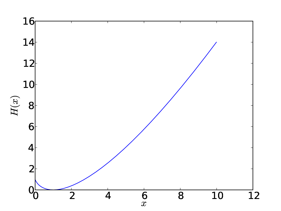
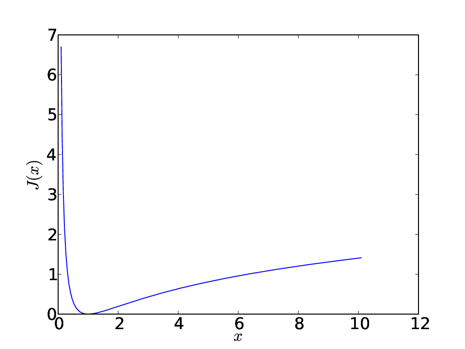
We first introduce the following functions upon which our analysis will heavily depend. For the function on (see Figure 4 left), define to be the inverse of on , and to be the inverse of on . Analogously for the function on (see Figure 4 right), define to be the inverse of on , and to be the inverse of on .
Theorem 2
Consider bootstrap percolation where and . For , and when
does not become fully active whp.
Proof We show that for the conditions of the assertion, an initial configuration is stable. The number of active nodes in the initial configuration follows Poisson distribution . The degree distribution of a node is , and the expected degree . By the thinning theorem [22] the number of active neighbors in the initial configuration follows . Consider the activation rule in . The probability that a node becomes active at the next time step given that it is inactive initially is .
For , given that , the tail bound on a Poisson random variable (10) implies for any node . Hence an initial configuration becomes fully active at the next time step with probability . Therefore we consider the case and seek a maximal (see Figure 3) such that does not become fully active whp. It follows
| (1) |
The same inequality (10) yields that the number of nodes within the square is concentrated around its mean whp. Hence the union bound over all nodes provides
| (2) |
Given , the condition suffices that the initial configuration is stable whp. The function is monotonically decreasing on , monotonically increasing on , with the minimum attained at . Hence for any positive there are two solutions of , denoted . This yields or . The acceptable solution is , since we consider the case . For from (2) it follows the probability that the initial configuration is stable tends to one as tends to infinity. Finally, a bound on is given by
which concludes the proof.
The following result clarifies the feasible region for and in Theorem 4.
Lemma 3
The condition is equivalent to:
and
Proof By inspection of the function .
Theorem 4
Consider bootstrap percolation where , , and . When and for
becomes fully active within steps whp.
For an initial configuration becomes fully active at the next time step whp (see the proof of Theorem 2), therefore we consider the case .
The proof of Theorem 4 consists of two parts. We tile the square into cells and show that in the initial configuration: (i) When , , and , every cell contains at least nodes whp; (ii) When at least one cell contains or more active nodes. By Lemma 1 it follows that for in the specified ranges becomes fully active within steps whp.
Proof Tile the square into cells , see Figure 5. Define the area of a cell . Call two cells neighboring if they share one side. Notice every pair of nodes within the same cell or within two neighboring cells are adjacent by the choice of the size of a cell. Define on the set of nodes of as follows. The set of edges of consists of the subset of edges of whose terminal nodes belong to the same cell or two neighboring cells. Then the monotonicity of bootstrap percolation yields
| (3) |
Therefore it is sufficient to show that whp becomes fully active when (8).

Part (i) (To show that every cell contains at least nodes whp.) We first bound the probability that an arbitrary cell contains at most nodes. The number of nodes in a cell follows , i.e., . Moreover, the numbers of nodes in cells are independent random variables (given the Poisson point process ). For , from (10) we obtain
The total number of cells in is . The union bound taken over all cells yields
| (4) |
Finally, for , from (4) it follows that every cell contains at least nodes whp.
Part (ii). (To show that at least one cell contains or more active nodes.) We now derive conditions such that at least one cell contains at least active nodes in the initial configuration. In order to guarantee that whp there is at least one cell among , which contains at least active nodes in the initial configuration, it suffices to find such that
| (5) |
since
Define , then by rewriting (5) we need such that
| (6) |
By the Bahadur-Rao tail bound [3], as , i.e., , the shifted Poisson random variable satisfies
where the rate function is defined by
(See Appendix for the details.) Therefore for (6) to be satisfied we require
| (7) |
The left hand side of (7) equals
which is if . Given , the condition is equivalent to , and moreover to
| (8) |
To complete the proof notice that once any nodes within a cell become active, all nodes within that cell become active at the next time step as would all nodes within its neighboring cells. This resulting process which jointly activates all nodes within one cell is equivalent to activating a site in . The resulting BP in has the threshold by construction, see Figure 5. Thus becomes fully active when by Lemma 1. The proof follows from (3).
Remark 1
For non-trival percolation threshold, that is, , it is necessary
Remark 2
3.2 Analysis of Bounds on Critical Thresholds
The critical threshold can be rewritten as
| (9) |
The function is monotonically decreasing in , hence is monotonically increasing in and monotonically decreasing in . As an example we numerically compute and tabulate for and different values of in Table 1. In Figure 6, is plotted as a function of for different values of
| 3 | 0.0000234198 | 0.0003678767 |
|---|---|---|
| 4 | 0.0001242460 | 0.0019516511 |
| 5 | 0.0003391906 | 0.0053279940 |
| 6 | 0.0006649716 | 0.0104453500 |
| 7 | 0.0010794693 | 0.0169562642 |
| 8 | 0.0015576467 | 0.0244674579 |
| 9 | 0.0020779022 | 0.0326396121 |
| 10 | 0.0026234549 | 0.0412091329 |
| 25 | 0.0101188498 | 0.1589465210 |
| 50 | 0.0174952121 | 0.0174952120 |
| 100 | 0.0246619916 | 0.3873896589 |

The experiments are performed on with and nodes, and for the cases: (i) and , and (ii) and . On these instances of graphs, for each chosen value of in we simulate BP times. More precisely, within each experiment we generate a random initial configuration with the probability and perform BP with the threshold where the expected degree is calculated for a given input .
Numerical results are presented with the initial probability on the horizontal axis, and the percentage of fully active stable configurations on the vertical axis. Four cases when , , for , are presented in Figures 7, 8, 9 and 10, respectively. These charts match the bounds derived theoretically for and . Further, they appear to support the case that even though we do not currently have a proof one way or the other.


Acknowledgements
This work was funded by NIST Grant No. 60NANB10D128.
References
- [1] Aizenman, M., and Lebowitz, J. L. Metastability effects in bootstrap percolation. Journal of Physics A: Mathematical and General 21, 19 (1988), 3801–3813.
- [2] Amini, H. Bootstrap percolation and diffusion in random graphs with given vertex degrees. Electronic Journal of Combinatorics 17, #R25 (2010).
- [3] Bahadur, R. R., and Rao, R. R. On deviations of the sample mean. Ann. Math. Statist. 31, 4 (1960), 1015–1027.
- [4] Balogh, J., Bollobás, B., Duminil-copin, H., and Morris, R. The sharp threshold for bootstrap percolation in all dimensions. In preparation.
- [5] Balogh, J., Peres, Y., and Pete, G. Bootstrap percolation on infinite trees and non-amenable groups. Combinatorics, Probability & Computing 15, 5 (2006), 715–730.
- [6] Balogh, J., and Pittel, B. Bootstrap percolation on the random regular graph. Random Structures & Algorithms 30, 1-2 (2007), 257–286.
- [7] Bucklew, J. A. Large Deviation Techniques in Decision, Simulation, and Estimation. Wiley-Interscience, New York, 1990.
- [8] Cerf, R., and Cirillo, E. N. M. Finite size scaling in three-dimensional bootstrap percolation. Ann. Prob 27 (1998).
- [9] Chalupa, J., Leath, P. L., and Reich, G. R. Bootstrap percolation on a Bethe lattice. J. Phys. C 12, L31 (1979).
- [10] Erdős, P., and Rényi, A. On random graphs. Publ. Math. Inst. Hungar. Acad. Sci. (1959).
- [11] Erdős, P., and Rényi, A. On the evolution of random graphs. Publ. Math. Inst. Hungar. Acad. Sci. (1960).
- [12] Gersho, A., and Mitra, D. A simple growth model for the diffusion of new commuinication services. IEEE Trans. on Systems, Man, and Cybernetics SMC-5, 2 (March 1975), 209–216.
- [13] Gilbert, E. N. Random graphs. Ann. Math. Statist. 30, 4 (1959), 1141–1144.
- [14] Gilbert, E. N. Random plane networks. Soc. Ind. Appl. Math. 9, 4 (1961), 533–543.
- [15] Goel, A., Rai, S., and Krishnamachari, B. Sharp thresholds for monotone properties in random geometric graphs. In STOC ’04: Proceedings of the thirty-sixth annual ACM symposium on Theory of computing (New York, NY, USA, 2004), ACM Press, pp. 580–586.
- [16] Gupta, P., and Kumar, P. R. Critical power for asymptotic connectivity. In Proceedings of the 37th IEEE Conference on Decision and Control (1998), vol. 1, pp. 1106–1110.
- [17] Holroyd, A. E. Sharp metastability threshold for two-dimensional bootstrap percolation. Probability Theory and Related Fields 125 (2003), 195–224.
- [18] Kong, Z., and Yeh, E. M. Analytical lower bounds on the critical density in continuum percolation. In Proceedings of the Workshop on Spatial Stochastic Models in Wireless Networks (SpaSWiN) (Limassol, Cyprus, April 16, 2007.).
- [19] Luczak, T., Janson, S., Turova, T., and Vallier, T. Bootstrap percolation on the random graph . Ann. of Appl. Probab. To appear.
- [20] Meester, R., and Roy, R. Continuum percolation. Cambridge University Press, 1996.
- [21] Penrose, M. D. The longest edge of the random minimal spanning tree. The Annals of Applied Probability 7, 2 (1997), 340–361.
- [22] Penrose, M. D. Random Geometric Graphs. Oxford University Press, 2003.
- [23] Pottie, G. J., and Kaiser, W. J. Wireless integrated network sensors. Commun. ACM 43, 5 (2000), 51–58.
- [24] Rintoul, M. D., and Torquato, S. Precise determination of the critical threshold and exponents in a three-dimensional continuum percolation model. Journal of Physics A. Mathematical and General 30, 16 (1997), L585–L592.
- [25] Watts, D. J. A simple model of global cascades in random networks. Proceedings of the National Academy of Sciences 99 (2002), 5766–5771.
Appendix
Lemma 5
(Concentration on a Poisson random variable, see [22]). A Poisson random variable (with ) satisfies:
| (10) | |||||
| (11) |
where for .
Theorem 6
(Bahadur-Rao, see [7]) Let be an i.i.d. sequence of random variables such that and for all . If is of lattice type and , then
where attained at , and .
Claim 7
A Poisson random variable for satisfies
where for .
Proof Let for be the independent lattice type random variables. We have and . Consider: (i) the moment generating function , (ii) the rate function which is attained at , and (iii) the variance . Now the claim follows from Theorem 6.