We consider a system whose classical phase space is $\mathbb{R}^{2}=\left\{(x,p)\right\}$ with the Poisson bracket $\{x,p\}=1$ and the Hamiltonian

We assume the potential $V$ to be defined for all $x$ and real-valued.

The polymer Hilbert space is spanned by the basis states

with the inner product

where the object on the right hand side is the Kronecker delta. The position operator $\hat{x}$ acts by pointwise multiplication as

and the family of translation operators $\bigl\{\widehat{U}_{\mu}\mid\mu\in\mathbb{R}\bigr\}$ is defined as in Schrödinger quantization by

In Schrödinger quantization the action of $\widehat{U}_{\mu}$ (2.6) is weakly continuous in $\mu$, and the usual momentum operator $\hat{p}:=-i\partial_{x}$ can be defined in terms of the translation operator by $\widehat{U}_{\mu}=e^{i\mu\hat{p}}$. In polymer quantization the action of $\widehat{U}_{\mu}$ is not weakly continuous in $\mu$ and a similar definition of a momentum operator is not available. Instead, we now take $\mu$ to be a fixed positive constant, understood as a fundamental length scale in the polymer quantum theory, and define the momentum operator and its square by

where ${\bar{\mu}}:=2\mu$. The polymer Hamiltonian is defined to be

where $\widehat{V}$ acts by pointwise multiplication,

and

$\widehat{H}$ is clearly symmetric. Its action decomposes the polymer Hilbert space into a continuum of separable superselection sectors, where each sector consists of wave functions supported on the regular ${\bar{\mu}}$-spaced lattice $\left\{\Delta+m{\bar{\mu}}\mid m\in\mathbb{Z}\right\}$ and the parameter $\Delta\in[0,{\bar{\mu}})$ parametrizes the sectors. A study of the deficiency indices [1] shows that $\widehat{H}$ has at least one self-adjoint extension in each superselection sector. In particular, the Kato-Rellich theorem [1] can be applied as in [10] to show that $\widehat{H}$ is essentially self-adjoint in every superselection sector in which the function $V$ is bounded.

It is useful to write the Hilbert space of each superselection sector in terms of sequences. For concreteness, consider the superselection sector $\Delta=0$. An orthonormal basis is given by $\bigl\{\psi_{m{\bar{\mu}}}\mid m\in\mathbb{Z}\bigr\}$. Writing $\psi=\sum_{m}c_{m}\psi_{m{\bar{\mu}}}$, the inner product reads $\left(\psi^{(1)},\psi^{(2)}\right)=\sum_{m}\overline{{c_{m}}^{(1)}}\,c_{m}^{(2)}$, and the action of $\widehat{H}$ reads

The Hilbert space hence consists of the two-sided square summable sequences $c:={(c_{m})}_{m=-\infty}^{\infty}$, and the action of $\widehat{H}$ reads

We wish to modify the polymer Hamiltonian (2.12) into a Hamiltonian in the Hilbert space of one-sided square-summable sequences.

We take the one-sided sequences to be of the form $c:={(c_{m})}_{m=1}^{\infty}$ and the inner product to read $\left(d,c\right)=\sum_{m=1}^{\infty}\overline{d_{m}}\,c_{m}$. We define the one-parameter family of modified Hamiltonians $\bigl\{\widehat{H}_{\alpha}\mid\alpha\in\mathbb{R}\bigr\}$ by

Each $\widehat{H}_{\alpha}$ is symmetric, and it can be verified as with the two-sided sequences that each $\widehat{H}_{\alpha}$ has at least one self-adjoint extension. If $V=0$, it can be explicitly verified that there are no nonvanishing normalizable solutions to $\widehat{H}_{\alpha}c=\pm ic$, and in this case $\widehat{H}_{\alpha}$ is hence essentially self-adjoint. It follows by the Kato-Rellich theorem [1] that $\widehat{H}_{\alpha}$ is essentially self-adjoint whenever the set $\bigl\{V(m{\bar{\mu}})\mid m=1,2,\ldots\bigr\}$ is bounded.

The motivation for the definition of $\bigl(\widehat{H}_{\alpha}c\bigr)_{m}$ by (2.13) is that $\bigl(\widehat{H}_{\alpha}c\bigr)_{m}$ agrees with $\bigl(\widehat{H}c\bigr)_{m}$ (2.12) for $m\geq 1$ if we envisage there to be a fictitious lattice point at $m=0$ such that $c_{0}=\alpha c_{1}$. This means that $\alpha\in\mathbb{R}$ can be regarded as a lattice counterpart of the continuum theory self-adjoint extension parameter $L$. The case $\alpha=0$ is analogous to continuum Dirichlet, with the continuum boundary at $m=0$. The cases $\alpha=\pm 1$ are respectively analogous to the continuum Neumann and continuum Dirichlet, with the continuum boundary half-way between $m=0$ and $m=1$.

Two comments are in order. First, given the definition (2.13), the coefficient of $\overline{d_{1}}\,c_{1}$ in the inner product $\left(d,c\right)=\sum_{m=1}^{\infty}\overline{d_{m}}\,c_{m}$ cannot be changed without losing symmetricity of $\widehat{H}_{\alpha}$. Second, although the definition of $\widehat{H}_{\alpha}$ is motivated by a fictitious lattice point at $m=0$, the actual definition involves $V$ only at lattice points $x=m{\bar{\mu}}$ with $m\geq 1$. $\widehat{H}_{\alpha}$ is hence well defined even if the classical potential is singular at $x=0$.

In Schrödinger quantization, the Hamiltonian operator of a free particle on the half-line is $\widehat{H}_{\text{free}}:=-d^{2}/dx^{2}$, acting in the Hilbert space $L_{2}(\mathbb{R}_{+},dx)$. $\widehat{H}_{\text{free}}$ is symmetric and has a $\text{U(1)}\simeq S^{1}$ of self-adjoint extensions, specified by the boundary condition (1.1).

The spectrum of each extension contains the positive continuum. The extensions with $0<L<\infty$ have in addition a discrete ground state of energy $-L^{-2}$. The spectral decomposition of the identity in terms of the eigenfunctions can be found in [18].

Polymer quantization on the full real line can be analyzed by interpreting the two-sided square summable sequence $c:={(c_{m})}_{m=-\infty}^{\infty}$ as the coefficients in the Fourier expansion $\chi(\varphi)={(2\pi)}^{-1/2}\sum_{m}c_{m}e^{im\varphi}$ of the function $\chi\in L_{2}(S^{1})$, so that in this realization $\bigl(\widehat{H}\chi\bigr)(\varphi)=2{\bar{\mu}}^{-2}\left(1-\cos\varphi\right)\chi(\varphi)$. It is immediate that $\widehat{H}$ is essentially self-adjoint and its spectrum is the continuum $(0,4{\bar{\mu}}^{-2})$.

The half-line polymer Hamiltonian is given by $\widehat{H}_{\alpha}$ (2.13) with $V=0$. As noted above, $\widehat{H}_{\alpha}$ is essentially self-adjoint.

In Schrödinger quantization [20], the Hamiltonian has a one-parameter family of self-adjoint extensions, specified by a boundary condition at $x=0$. The boundary condition does not take the Robin form (1.1) but reads instead

where $\psi$ is the wave function, $\Psi$ is the digamma function [21] and ${\tilde{L}}\in\mathbb{R}\cup\{\infty\}$ is the parameter. The second term in (4.1) can be understood as a logarithm-corrected first derivative, where the correction must be included because of the singularity of the potential at $x\to 0$.

The spectrum consists of the positive continuum and a countable number of proper negative eigenvalues. Writing $s:=1/\sqrt{-4E}$ for $E<0$, the eigenvalues are given by the solutions to

The solutions to (4.2) with ${\tilde{L}}=\infty$ are $s=1,2,3,\ldots$, coming from the simple poles of $\Psi$ at non-positive integers. This extension is analogous to the Dirichlet boundary condition for regular potentials, and it arises via a limiting prescription from regularized potentials that make the three-dimensional attractive Coulomb Hamiltonian essentially self-adjoint [20]. This is the extension that yields the textbook spectrum, realized in nature.

We note in passing that if physical dimensions are restored, ${\tilde{L}}$ has an interpretation as an inverse length scale. Using ${\tilde{L}}$, rather than the associated length scale $1/{\tilde{L}}$ [20], is convenient for us because the spectrum changes smoothly across ${\tilde{L}}=0$. The only discontinuous change in the spectrum in terms of ${\tilde{L}}$ occurs when ${\tilde{L}}\to\infty$ through positive values: in this limit the ground state descends to $-\infty$ and disappears.

The half-line polymer Hamiltonian is given by $\widehat{H}_{\alpha}$ (2.13) with $V(m{\bar{\mu}})=-1/(m{\bar{\mu}})$. As noted in subsection 2.2, the boundedness of $V$ over the lattice points shows that $\widehat{H}_{\alpha}$ is essentially self-adjoint.

We focus on a numerical study of the proper eigenvalues in the limit ${\bar{\mu}}\to 0$. The numerical scheme is as described in [9] except that the boundary condition to shoot for is now $c_{0}=\alpha c_{1}$.

The key is again to make $\alpha$ depend on ${\bar{\mu}}$ in a suitable way. Motivated by the continuum boundary condition (4.1), we introduce a parameter ${{\tilde{L}}_{P}}\in\mathbb{R}\cup\{\infty\}$, and we choose

which is well defined for sufficiently small ${\bar{\mu}}$ with any fixed value of ${{\tilde{L}}_{P}}$. Numerical results for the lowest three eigenvalues in terms of ${{\tilde{L}}_{P}}$ are shown in Table 1. Numerical accuracy allows us to probe values of ${\bar{\mu}}$ down to $10^{-5}$.

For ${{\tilde{L}}_{P}}=\infty$, we find that the polymer eigenenergies converge to those of the Schrödinger theory with ${\tilde{L}}=\infty$. For other values of ${{\tilde{L}}_{P}}$, we find that the polymer eigenenergies converge to those of a Schrödinger theory with ${\tilde{L}}-{{\tilde{L}}_{P}}\approx 0.423$. While we do not have an analytic explanation for this shift in ${\tilde{L}}-{{\tilde{L}}_{P}}$, we note that within our numerical accuracy the shift coincides with the constant $\Psi(2)\approx 0.4227843351$ that appears in (4.1) and (4.3). Examining whether this coincidence continues to hold beyond three decimal places would require numerical work beyond ${\bar{\mu}}=10^{-5}$.

If the limit ${\bar{\mu}}\to 0$ is taken with any fixed value of $\alpha$, the relation (4.3) shows that the numerical results in Table 1 are consistent with convergence to the continuum theory with ${\tilde{L}}=\infty$.

Schrödinger quantization of the system is reviewed in [10]. For $\lambda\leq-3/4$ the Hamiltonian is essentially self-adjoint and the spectrum consists of the positive continuum. For $\lambda>-3/4$ the self-adjoint extensions are specified by a parameter that takes values in $\text{U}(1)\simeq S^{1}$, and the spectrum of each extension contains the positive continuum but discrete negative eigenenergies can also exist. We shall recall here relevant facts about the cases in which discrete eigenenergies do exist.

For $\lambda>1/4$, each extension has a countable tower of proper eigenenergies, given by

where $\gamma\in[0,\pi)$ is the parameter specifying the extension. The discrete spectrum is unbounded below, $E_{n}\to-\infty$ as $n\to-\infty$, and it accumulates to $0$ from below, $E_{n}\to 0_{-}$ as $n\to\infty$.

For $\lambda=1/4$, one of the extensions has no discrete eigenenergies but the rest have exactly one negative eigenenergy each.

For $-3/4<\lambda<1/4$, there is an open interval of extensions that have exactly one negative eigenenergy each. The remaining extensions have no discrete eigenenergies.

The half-line polymer Hamiltonian is given by $\widehat{H}_{\alpha}$ (2.13) with $V(m{\bar{\mu}})=-\lambda/(m{\bar{\mu}})^{2}$. The boundedness of $V$ over the lattice points again implies that $\widehat{H}_{\alpha}$ is essentially self-adjoint.

We again focus on a numerical study of the discrete eigenvalues. Because of the scale invariance of the potential, the polymer eigenvalues depend on ${\bar{\mu}}$ only through the overall factor ${\bar{\mu}}^{-2}$. The question to be examined hence is how the combination ${\bar{\mu}}^{2}E$ depends on $\lambda$.

Because of the strong singularity of the continuum potential at $x\to 0$, it is not clear how the Schrödinger theory self-adjointness boundary conditions [10] might motivate a value of $\alpha$ in our polymer Hamiltonian. We hence take $\alpha=\tan\chi$, where $\chi\in[0,\pi)$, allowing $\chi=\pi/2$ to be considered as a limiting case. The numerical implementation is as in [10] except that the boundary condition to shoot for is

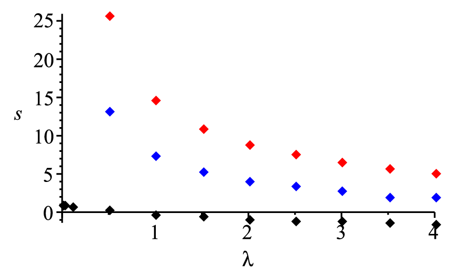
For $\lambda\gtrsim 2$, we find a tower of negative eigenenergies $E_{0}<E_{1}<E_{2}<\cdots<0$. We have followed the tower up to $E_{6}$ but slowness of the numerics has not enabled us to examine whether the tower terminates. Starting at $\chi=0$ and increasing $\chi$, $E_{0}$ first migrates downwards and then disappears at $\chi\approx\pi/2$; slowness of the numerics has not enabled us to examine whether this disappearance happens by descent to $-\infty$ or by some other mechanism. The excited states $E_{n}$, $n>0$, migrate down smoothly, meeting at $\chi\to\pi$ with $E_{n-1}$ at $\chi=0$. Graphs for $E_{3}$ in terms of $\chi$ are shown in Figure 1 for $\lambda=4$ and $\lambda=8$.

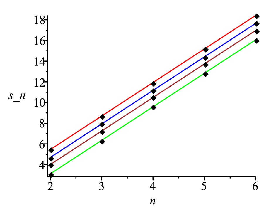
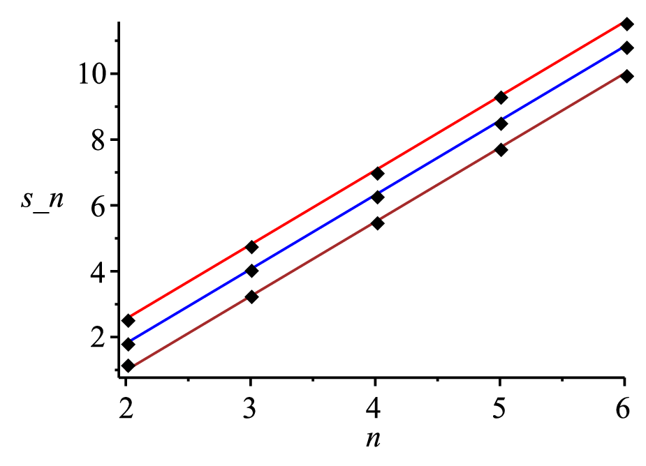
When $\lambda$ decreases towards $0$, the numerics becomes slow. Outside the interval $\pi/4<\chi<\pi/2$ we have found no evidence that any eigenstates would survive. Within the interval $\pi/4<\chi<\pi/2$, however, comparison with the free particle polymer theory of Section 3 suggests that the ground state should persist as $\lambda\to 0$ and tend to that of the corresponding $\lambda=0$ theory, given by

and we find numerical evidence that this indeed happens. A sample plot is shown in Figure 2.

If the lowest few states are excluded, the eigenergies for $\lambda\gtrsim 2$ are a good fit to the continuum eigenenergy formula (5.1), as shown in Figure 3. The continuum parameter $\gamma$ is an increasing function of $\chi$, and for large $\lambda$ it is slowly varying except when $\chi$ is close to $\pi/2$.

Following [11], we take the classical phase space to be $({\phi},\Pi)$, where the positive-valued configuration coordinate ${\phi}$ is the square of the wormhole throat area-radius and $\Pi$ is the real-valued conjugate momentum. The classical Hamiltonian is given by

We take the wave functions in Schrödinger quantization to be square integrable functions of ${\phi}$ in the measure $d{\phi}$. For reasons that will emerge in the polymer theory, we consider the quantum Hamiltonian with the symmetric ordering

It is shown in [11, 24] that the self-adjoint extensions of $\widehat{H}_{\text{Schr}}$ are labelled by the parameter $\theta\in[0,\pi)$ such that

or equivalently

so that $\theta=0$ is analogous to Dirichlet and $\theta=\pi/2$ is analogous to Neumann. The spectrum of each self-adjoint extension is discrete and bounded below. Further analytic and numerical results on the spectrum are given in [11, 24].

As the kinetic term of the classical Hamiltonian (6.1) does not have the conventional form of (2.1), the polymer quantization prescription of Section 2 must be suitably generalized. We now recall the results of [11] for the situation where ${\phi}$ is polymer quantized on the full real line.

We polymerize the pair $({\phi},\Pi)$ as the pair $(x,p)$ in subsection 2.1, letting ${\phi}$ take all real values, defining the basis states

with the inner product

and the operators

where the positive constant $\mu$ is again the fundamental polymer length scale. The polymer counterpart of the Schrödinger Hamiltonian (6.9) is taken to be

where the operator $\hat{\phi}^{1/2}$ is defined by

Specialising to the superselection sector in which ${\phi}$ is confined to the lattice $\bigl\{m{\bar{\mu}}\mid m\in\mathbb{Z}\bigr\}$ with ${\bar{\mu}}:=2\mu$, and writing $\psi=\sum_{m}c_{m}\psi_{m{\bar{\mu}}}$, the action of $\widehat{H}$ on the two-sided square-summable sequence $c:={(c_{m})}_{m=-\infty}^{\infty}$ reads

It follows that the polymer Hilbert space breaks further into the even superselection sector, in which $c_{m}=c_{-m}$, and the odd superselection sector, in which $c_{m}=-c_{-m}$. In the limit ${\bar{\mu}}\to 0$, it is found numerically [11] that the even (respectively odd) sector converges to the Schrödinger theory with $\theta=\pi/2$ ($\theta=0$). This convergence is consistent with what one would expect by inspection of the Schrödinger theory boundary condition (6.3).

References

- [1] M. Reed and B. Simon, Methods of Modern Mathematical Physics II: Fourier Analysis, Self-adjointness (Academic, New York, 1975).
- [2] J. Blank, P. Exner and M. Havlíček, Hilbert Space Operators in Quantum Physics, 2nd edition (Springer, New York, 2008).
- [3] G. Bonneau, J. Faraut and G. Valent, “Self-adjoint extensions of operators and the teaching of quantum mechanics”, Am. J. Phys. 69, 322 (2001) [arXiv:quant-ph/0103153]; V. S. Araujo, F. A. B. Coutinho and J. F. Perez, “Operator domains and self-adjoint operators”, Am. J. Phys. 72, 203 (2004); T. Fülöp, “Singular potentials in quantum mechanics and ambiguity in the self-adjoint Hamiltonian”, SIGMA 3, 107 (2007) [arXiv:0708.0866 [quant-ph]].
- [4] B. Belchev and M. A. Walton, “Robin boundary conditions and the Morse potential in quantum mechanics”, J. Phys. A 43, 085301 (2010) [arXiv:1002.2139 [quant-ph]].
- [5] A. Ashtekar, S. Fairhurst and J. Willis, “Quantum gravity, shadow states, and quantum mechanics”, Class. Quant. Grav. 20, 1031 (2003) [arXiv:gr-qc/0207106].
- [6] H. Halvorson, “Complementarity of representations in quantum mechanics”, Studies Hist. Philos. Mod. Phys. 35, 45 (2004) [arXiv:quant-ph/0110102].
- [7] T. Thiemann, Modern Canonical Quantum General Relativity (Cambridge University Press, Cambridge, 2007).
- [8] C. Rovelli, Quantum Gravity (Cambridge University Press, Cambridge, 2007).
- [9] V. Husain, J. Louko and O. Winkler, “Quantum gravity and the Coulomb potential”, Phys. Rev. D 76, 084002 (2007) [arXiv:0707.0273 [gr-qc]].
- [10] G. Kunstatter, J. Louko and J. Ziprick, “Polymer quantization, singularity resolution and the potential”, Phys. Rev. A 79, 032104 (2009) [arXiv:0809.5098 [gr-qc]].
- [11] G. Kunstatter, J. Louko and A. Peltola, “Polymer quantization of the Einstein-Rosen wormhole throat,” Phys. Rev. D 81, 024034 (2010) [arXiv:0910.3625 [gr-qc]].
- [12] G. Kunstatter, J. Louko and A. Peltola, “Quantum dynamics of the Einstein-Rosen wormhole throat,” Phys. Rev. D 83, 044022 (2011) [arXiv:1010.3767 [gr-qc]].
- [13] T. Thiemann, “Quantum spin dynamics (QSD),” Class. Quant. Grav. 15, 839 (1998) [arXiv:gr-qc/9606089].
- [14] G. Chacon-Acosta, E. Manrique, L. Dagdug and H. A. Morales-Tecotl, “Statistical thermodynamics of polymer quantum systems,” SIGMA 7, 110 (2011) [arXiv:1109.0803 [gr-qc]].
- [15] E. Marinari and G. Parisi, “On polymers with long-range repulsive forces,” Europhys. Lett. 15, 721 (1991).
- [16] J.-M. Lévy-Leblond, “Electron capture by polar molecules,” Phys. Rev. 153, 1 (1967); O. H. Crawford, “Bound states of a charged particle in a dipole field,” Proc. Phys. Soc. (London) 91, 279 (1967); C. Desfrançois, H. Abdoul-Carime, N. Khelifa and J. P. Schermann, “From to potentials: Electron exchange between Rydberg atoms and polar molecules,” Phys. Rev. Lett. 73, 2436 (1994).
- [17] J. Gegenberg, G. Kunstatter and R. D. Small, “Quantum structure of space near a black hole horizon,” Class. Quant. Grav. 23, 6087 (2006) [gr-qc/0606002]; G. Kunstatter and J. Louko, “Transgressing the horizons: Time operator in two-dimensional dilaton gravity,” Phys. Rev. D 75, 024036 (2007) [gr-qc/0608080].
- [18] E. C. Titchmarsh, Eigenfunction Expansions, Vol. I, 2nd edition (Clarendon, Oxford, 1962).
- [19] S. Odake and R. Sasaki, “Discrete quantum mechanics,” J. Phys. A 44, 353001 (2011).
- [20] C. J. Fewster, “On the energy levels of the hydrogen atom,” arXiv:hep-th/9305102.
- [21] Digital Library of Mathematical Functions (National Institute of Standards and Technology, Gaithersburg, Maryland, USA, 2010), http://dlmf.nist.gov/ .
- [22] J. L. Friedman, I. H. Redmount, and S. N. Winters-Hilt (unpublished, 1993).
- [23] I. H. Redmount, talk given at the 3rd Midwest Relativity Meeting, Oakland, Michigan, 1993.
- [24] J. Louko and J. Mäkelä, “Area spectrum of the Schwarzschild black hole”, Phys. Rev. D 54, 4982 (1996) [arXiv:gr-qc/9605058].
- [25] M. Bojowald, “Loop quantum cosmology,” Living Rev. Rel. 8, 11 (2005) [gr-qc/0601085].
- [26] A. Ashtekar and P. Singh, “Loop quantum cosmology: a status report,” Class. Quant. Grav. 28, 213001 (2011) [arXiv:1108.0893 [gr-qc]].
- [27] G. M. Hossain, V. Husain and S. S. Seahra, “Background independent quantization and wave propagation,” Phys. Rev. D 80, 044018 (2009) [arXiv:0906.4046 [hep-th]].