Andreev quantum dot with several conducting channels

In the middle of the last century, Josephson showed that a nondissipative current can flow between two superconductors separated by an intermediate region when a phase difference is applied between the two superconductors.[1, 2, 3] This intermediate region can, in practice, be composed of an insulator, a normal metal, a constriction, etc. Recent developments of nanotechnology allow us to insert quantum dots, e.g., using carbon nanotubes [4, 5] in this region. These types of Josephson junctions are called Andreev quantum dots.[6, 7] The charge of the Andreev dot was shown to vary smoothly with the phase difference between the superconductors[7, 8] in the absence of Coulomb interaction.

Reference 7 showed that the charge could be tuned continuously from $0$ to $2e$ depending on the phase difference $\varphi$ and gate voltage $V_{\rm g}$. In Refs. 9 and 10 it was shown that the Coulomb interaction can change the property of the ground state, from a usual nondegenerate state with two quasiparticles to a doubly degenerate state with one quasiparticle. The present article is a logical continuation of the above-mentioned work and is devoted to the case of several channels. These channels may appear due to the presence of two orbits in a single-wall carbon nanotubes and in multiwall nanotubes[11], or due to an inhomogeneous distribution of transverse quantized energy levels in metal wires.[12] In this article, we answer the natural questions: How is the charge dependence on the phase difference affected by the presence of such channels, what is the effect of Coulomb interaction between channels, and how does this dependence scale with the number of channels? The calculation is done in the limit of a large superconducting gap.

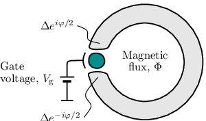
We describe the ground state properties for different setups with different strengths of the regular Andreev reflection (AR)[13] and crossed Andreev reflection (CAR)[14, 15, 16, 17] for different types of Coulomb interaction, such as metal nanowires with $1$ channel, single-wall carbon nanotubes (SWNT) with $2$ orbital channels, multiwall carbon nanotubes (MWNT) with $4$ channels, and two separate SWNTs with $2\times 2$ channels. In this article, we mainly focus on the dependencies on the tunable parameters gate voltage and superconducting phase difference. We consider the interplay between phase-sensitive singlet (nondegenerate) and phase-insensitive doubled (doubly degenerate) states from different channels, study the current-to-gate voltage and charge-to-phase sensitivities, and discuss two applications, the Josephson transistor[18] and a magnetometer based on an Andreev quantum dot.[10]

In Sec. II, we describe a setup based on a quantum dot with several levels, or alternatively an intermediate region composed of several single-wall nanotubes/a multiwall nanotube. The model Hamiltonian is introduced in Sec. III. In Sec. IV, we represent the iterative scheme providing the matrix elements of the $N$-channel Hamiltonian. Using these results, we study the degeneracy and energy of the ground state as a function of the superconducting phase difference and gate voltage in Sec. V. Furthermore, we analyze the magnetic properties of the dot in Sec. VI. The charge on the dot and the Josephson current are calculated in Sec. VII, and their “sensitivities” are discussed in Sec. VIII.

As shown in Fig. 1, the setup consists of a structured Josephson junction in the form of an Andreev quantum dot inserted into a superconducting loop. We consider a quantum dot with one or several conducting channels and account for the Coulomb interaction and crossed Andreev reflection. In the Andreev dot without Coulomb interactions, strong normal reflection (electron$\,\to\,$electron, hole$\,\to\,$hole) competes with Andreev reflection (electron$\,\to\,$hole, hole$\,\to\,$electron), and as a result a strong dependence of the charge and current on the superconducting phase difference occurs. Every conducting channel contributes to the charge[7] and current.[19, 18] Our Andreev dots describe a situation where the resonance width $\Gamma$ is much smaller than the superconducting gap $\Delta$ ($\Gamma\ll\Delta$) and the length of the normal part $L$ is much shorter than the superconducting coherence length $\xi$ ($L\ll\xi$). The superconducting phase difference $\varphi$ across the junction is controlled by the magnetic flux $\Phi$ passing through the ring: $\varphi=2\pi\Phi/\Phi_{0}$, where $\Phi_{0}$ is the flux quantum $\Phi_{0}=2|e|/2\pi\hbar$ and $e=-|e|$ is a charge of one electron.

Realistic experimental setups might be based on a single-wall nanotube,[4, 5] on two or more single-wall nanotubes placed in parallel, or on a multiwall nanotube. The case with two parallel single-wall nanotubes is illustrated in Fig. 2(b): This case is interesting because the Coulomb interaction between nanotubes can be smaller than in each nanotube. If such nanotubes are separated by a large distance, the effects of the tubes will be additive. The second interesting and experimentally realized case is the multiwall nanotube with approximately equal interactions in each channel and between them, as depicted in Fig. 2(c).

We consider a SWNT suspended between two superconducting leads, cf. Fig. 2(a). Additional gates placed above the nanotube allow us to define precisely the extent of the quantum dot and therefore allow us to modulate its energy levels. An overall gate voltage allows us to apply an electric field to the entire structure and changes the position of the normal dot levels $\varepsilon_{i}$ (index $i=1,\ldots,N$ labels the channels). The normal island(s) can be described as zero dimensional objects.

The model can be described by a Hamiltonian which includes the dot and its internal degrees of freedom, the leads, and the tunnel coupling between the latter two, ${\hat{H}}={\hat{H}}_{\rm\scriptscriptstyle D}+{\hat{H}}_{\rm\scriptscriptstyle S}+{\hat{H}}_{\rm\scriptscriptstyle T}$. The first part ${\hat{H}}_{\rm\scriptscriptstyle D}$ describes the quantum dot with $N$ normal levels

where the first term represents the interaction with the external gate, ${\hat{n}}_{i}={\hat{n}}_{i\uparrow}+{\hat{n}}_{i\downarrow}$, ${\hat{n}}_{i\sigma}={\hat{d}}_{i\sigma}^{\dagger}{\hat{d}}_{i\sigma}^{\phantom{{\dagger}}}$, and ${\hat{d}}_{i\sigma}^{\dagger}$ and ${\hat{d}}_{i\sigma}^{\phantom{{\dagger}}}$ are electronic creation and annihilation operators for the $i^{\text{th}}$ level in the dot, respectively; $\sigma=\uparrow,\downarrow$, and $\varepsilon_{i}$ is the $i^{\text{th}}$ energy level with respect to the Fermi level. The second term describes the Coulomb interaction within the channels ($U_{ii}$) and between different channels ($U_{ij}$, $i\neq j$). The symmetric matrix $U_{ij}$ is positive definite, and all its elements are positive.[20] The lead Hamiltonian describes two BCS superconductors [with a lead index $\ell=\rm L,R$ (left, right)]

with an energy dispersion in the superconducting leads $\xi_{k}=\hbar^{2}k^{2}/2m-E_{\rm\scriptscriptstyle F}$ and an absolute value of the gap $\Delta$ in the bulk of the superconductors. The electron hopping term between dots and leads is given by

where $\mathcal{\hat{T}}_{\rm\scriptscriptstyle L,R}=t_{\rm\scriptscriptstyle L,R}{\hat{\sigma}}_{z}e^{\pm i{\hat{\sigma}}_{z}\varphi/4}$ and $t_{\ell}$ are tunneling amplitudes between the superconductors and the dot. The superconductor has a phase $\varphi/2$ on the left and $-\varphi/2$ on the right. The calculation of observables for a thermal equilibrium system starts from the evaluation of the partition function $Z={\rm Tr}\{e^{-\beta{\hat{H}}}\}$, where $\beta$ is the inverse temperature.

We work in the limit of a large superconducting gap $|\varepsilon_{i}|$, $U_{ij}$, $\Gamma_{ij}\ll\Delta$ (the so-called $\Delta\to\infty$ limit), where $\Gamma_{ij}$ are the resonance half-widths originating from tunneling processes [Eq. (3)]. In this limit, one can integrate over the lead degrees of freedom and benefit from the absence of retardation effects due to the latter. The Hamiltonian $\hat{H}$ can be rewritten in a simpler form

describing the dot alone with the superconductors defining the boundary conditions.[21, 22, 23] We explicitly indicate the number of channels $N$ in the Hamiltonian $\mathcal{\hat{H}}_{\scriptscriptstyle N}$ [Eq. (4)] and build an iterative scheme for its matrix elements $\mathcal{H}_{\scriptscriptstyle N}$ on $N$. Upon integration, Eqs. (2) and (3) generate the last term in Eq. (4), which implies that this Hamiltonian does not conserve the number of electrons. The coefficients ${\tilde{\Gamma}}_{ij}$ are directly derived from the tunneling amplitudes $t_{\rm\scriptscriptstyle L,R}$ and describe two-particle tunneling processes involving both Andreev and normal scattering events at the left and right boundaries. For symmetric boundaries with equal transparencies $|t_{\rm\scriptscriptstyle L}|^{2}=|t_{\rm\scriptscriptstyle R}|^{2}=|t|^{2}$, we find $\tilde{\Gamma}_{ij}=\Gamma_{ij}\cos(\varphi/2)$. The symmetric matrix $\Gamma_{ij}$ describes Andreev reflection, the annihilation of two quasiparticles from the $i^{\text{th}}$ and $j^{\text{th}}$ channel ${\hat{d}}_{i\downarrow}{\hat{d}}_{j\uparrow}$ (with simultaneous creation of a Cooper pair in the superconductor) and the opposite process. The diagonal terms ${\tilde{\Gamma}}_{ii}$ correspond to the regular Andreev reflection inside the $i^{\text{th}}$ channel, the off-diagonal terms ${\tilde{\Gamma}}_{ij}$, ($i\neq j$)  describes the crossed Andreev reflection (CAR) between the $i^{\text{th}}$ and $j^{\text{th}}$ channel. The element $\Gamma_{ij}$ can be treated as the resonance half-width of the normal tunneling process between the $i^{\text{th}}$ and $j^{\text{th}}$ channel. Note that for a diagonal matrix $\Gamma_{ij}$ and $U_{ij}$ (with $\Gamma_{ij}=0$, $U_{ij}=0$, $i\neq j$) the channels are additive and the answers for all physical quantities can be obtained by summation over all channels.

The Hamiltonian Eq. (4) for a single channel (the first channel in the iterative scheme presented below) has the following form

where the $\hat{n}_{1\sigma}^{2}$ contributions from the sum ${\hat{n}}_{1}^{2}=(\hat{n}_{1\uparrow}+\hat{n}_{1\downarrow})^{2}$ has been absorbed in a shift of $\varepsilon_{1}$. We denote the Hamiltonian of the $i^{\text{th}}$ channel as ${\hat{H}}_{i}$ and the total Hamiltonian of $N$ channels as $\mathcal{\hat{H}}_{\scriptscriptstyle N}$. The corresponding matrix of the $H_{1}$ Hamiltonian has dimensions $4\times 4$ and can be calculated in a basis of four states $|\nu\rangle_{1}=\{|0\rangle_{1}$, $|\!\!\uparrow\rangle_{1}$, $|\!\!\downarrow\rangle_{1}$, $|2\rangle_{1}\}$, the state with no electrons $|0\rangle$, with one electron with spin up $|\!\!\uparrow\rangle={\hat{d}}_{\uparrow}^{\dagger}|0\rangle$ or spin down $|\!\!\downarrow\rangle={\hat{d}}_{\downarrow}^{\dagger}|0\rangle$, and the two electron state $|2\rangle={\hat{d}}_{\uparrow}^{\dagger}{\hat{d}}_{\downarrow}^{\dagger}|0\rangle$

where

are matrix elements of the dimensionless charge operator and ${\hat{Q}}_{1}=e{\hat{n}}_{1}$. In what follows, the expression ${\rm adiag}\{x_{1},x_{2},\ldots,x_{\scriptscriptstyle N}\}$ stands for the $N\times N$ matrix $A_{ij}$, where $A_{i,N-i+1}=x_{i}$ and $A_{i,j}=0$ for $j\neq N-i+1$. The eigenvalues of Eq. (IV) can be easily calculated. They consist of two nondegenerate levels with energies

and a doubly degenerate level with energy

which can be split into two separate levels by an external magnetic field through the Zeeman effect. Usually, the ground state of the Hamiltonian Eq. (IV) is given by the singlet $E_{0}$. But in the case of nonzero Coulomb interaction $U_{1}>0$, there exists a range of parameters $\varphi$ and $\varepsilon_{i}$ for which the ground state is doubly degenerate with energy $E_{1}$. The doublet region is defined by the inequality

where ${\tilde{\varepsilon}}=\varepsilon_{1}+2U_{1}$. For an asymmetric dot ($|t_{\rm\scriptscriptstyle L}|\neq|t_{\rm\scriptscriptstyle R}|$), in the presence of electron-phonon interaction or other perturbations, the “critical” $U_{1}$ is different from zero, $U_{1,\rm\scriptscriptstyle C}>0$.[10] In this article, we ignore such nonidealities and concentrate on the simplest case. The same results are valid for any other $i>1$ channel; they can be obtained by the substitution $\varepsilon_{1}\to\varepsilon_{i}$, $\Gamma_{1}\to\Gamma_{i}$, and $U_{1}\to U_{i}$.

The structure of the ground state in the one-channel case is presented in Fig. 3 as a function of phase $\varphi$ and the “central” dot-level ${\tilde{\varepsilon}}=\varepsilon_{1}+2U_{1}$. The blue figures in the center represent the doublet state 12, their shapes are defined by the inequality (13), the white space around corresponds to a usual singlet state with energy (11). For two completely separated single-channel dots with the same levels $\varepsilon_{1}=\varepsilon_{2}$ connected in parallel, the dependence is the same, however, now the central figure corresponds to a four-fold degenerate situation.

We now go back to the $N$-channel case. We calculate the matrix elements of the Hamiltonian Eq. (4) in the basis $|\nu\rangle_{1}\otimes|\nu\rangle_{2}\otimes\ldots\otimes|\nu\rangle_{\scriptscriptstyle N}=\{{|0,\ldots,0\rangle},$ ${|0,\ldots,\uparrow\rangle},$ ${|0,\ldots,\downarrow\rangle},\ldots,$ ${|2,\ldots,\downarrow\rangle},$ ${|2,\ldots,2\rangle}\}$, where $|\nu\rangle_{i}=\{|0\rangle_{i}$, $|\!\!\uparrow\rangle_{i}$, $|\!\!\downarrow\rangle_{i}$, $|2\rangle_{i}\}$ are states of the Hamiltonian for the single channel case [Eq. (IV)]

Here, the first sum takes into account the interactions inside each channel (given by the direct tensor product of $H_{i}$’s and unity operators $\mathbbm{1}_{j}$ in the other subspaces). The second sum is the interaction between channels; each term represents the tensor product of the charge operator in the $i^{\text{th}}$ channel and in the $j^{\text{th}}$ channel [as given by Eq. (10)]. Here, $\mathbbm{1}_{i}$ is the unit matrix in the Hilbert subspace of the $i^{\text{th}}$ channel, and $Q_{i}$ is the matrix characterizing the $i^{\text{th}}$ channel charge. The third sum describes CAR; each term corresponds to the CAR in the $i^{\text{th}}$ and $j^{\text{th}}$ channels. The Coulomb interaction inside each channel and the regular Andreev reflection are accounted for in the first term.

Let us construct a recursive procedure in $N$ for the matrix elements corresponding to the $N$-channel Hamiltonian. As the initial step of the recursion $N=1$ we take the matrix (IV). At the second step $N=2$ we build a matrix in $|\nu\rangle_{1}\otimes|\nu\rangle_{2}$ in the following way:

where we keep in mind that ${\tilde{\Gamma}}_{12}={\tilde{\Gamma}}_{21}$. The matrices

and the corresponding Hermitian conjugates $d_{i\uparrow}^{\dagger}$, $d_{i\downarrow}^{\dagger}$ are the matrix elements of the operators ${\hat{d}}_{i\uparrow}^{\phantom{{\dagger}}}$, ${\hat{d}}_{i\downarrow}^{\phantom{{\dagger}}}$ and ${\hat{d}}_{i\uparrow}^{\dagger}$, ${\hat{d}}_{i\downarrow}^{\dagger}$ in the $i^{\text{th}}$ channel basis. This is a $16\times 16$ matrix (the Hilbert space of the $1^{\text{st}}$ channel with dimension 4 should be multiplied by the Hilbert space of the $2^{\text{nd}}$ one with the same dimension). Each “element” is a $4\times 4$ block, “diag” and “adiag” to be in the $2^{\text{nd}}$ channel subspace. $H_{1}$ originates from Eq. (IV), with scalar elements to be multiplied by $\mathbbm{1}_{1}$. The matrices $\mathbb{U}_{21}={\rm diag}_{1}\{0,0,0,8U_{12}\}$ and $\mathbb{U}_{22}={\rm diag}_{1}\{0,8U_{12},8U_{12},0\}$ are based on the term $U_{12}$ which is responsible for the interaction between channels. For the noninteracting case $U_{12}=0$, the structure of the ground state is presented in Fig. 4(a) [$\varepsilon_{2}-\varepsilon_{1}=0$] and 4(d) [$\varepsilon_{2}-\varepsilon_{1}=\Gamma$] in coordinates $(\varphi,\tilde{\varepsilon})$, where ${\tilde{\varepsilon}}=(\varepsilon_{1}+\varepsilon_{2})/2+U_{1}+U_{2}$ is the average and renormalized normal level in the dot. The interacting case is shown in Figs. 4(g) and 4(j), where ${\tilde{\varepsilon}}=(\varepsilon_{1}+\varepsilon_{2})/2+U_{1}+U_{2}+2U_{12}$; see Sec. V for more details.

In the same way we can write a recursive formula for $\mathcal{H}_{\scriptscriptstyle N}$. The easiest way to write it down is

Here each matrix with index $i$ should be written as a matrix of size $4^{i}\times 4^{i}$ (i.e., in the subspace of the $i^{\text{th}}$ channel). Herein each element of the matrix associated with the $i^{\text{th}}$ channel is multiplied by a unitary matrix of size $4^{i-1}\times 4^{i-1}$ and starts on column $(c-1)\,2^{i-1}+1$ and on row $(r-1)\,2^{i-1}+1$ of the total matrix, where $c=1,\ldots,4$ is the column and $r=1,\ldots,4$ is the row in the original $4\times 4$ matrix of the $i^{\text{th}}$ channel. Schematically the recursive procedure for building the $N$-channel matrix can be represented as (for $N=3$)

The smallest “rectangle” corresponds to the Hamiltonian $H_{1}$. In a second step, we insert such blocks in the Hamiltonian $H_{2}$ and continue the procedure till $N$. At each $i^{\text{th}}$ step, we multiply the current space by the Hilbert subspace of the $i^{\text{th}}$ Andreev level.

Note that the same procedure can be realized by using the Bogoliubov-de Gennes equations and the scattering matrix approach in the tunneling regime (with a transparency of each junction much less than unity) as was done in Ref. 10 for a single channel. However, this approach is poorly scalable with $N$ and the calculation is much more cumbersome. See also Ref. 24 for the correspondence between the tunneling Hamiltonian method and the scattering matrix approach.

In the present notation, the first, the second, and the fourth sum in Eq. (24) are diagonal. In the absence of superconductivity they define energy levels of the system, and the Coulomb interaction leads to level “repulsion.” The third term of Eq. (24) includes the dependence on the superconducting phase difference and mixes the states due to the presence of Cooper pairs in the superconductors. At $\varphi=\pi$ the Hamiltonian Eq. (24) is diagonal and its eigenvalues can be found analytically.

In the single channel case, the ground state is formed by nondegenerate [Eq. (11)] or doubly degenerate [Eq. (12)] levels. However, for a large number of channels one can expect to observe $2^{\mathcal{P}_{\scriptscriptstyle N}}$ degeneracy, where $\mathcal{P}_{\scriptscriptstyle N}$ is the number of Andreev levels in the doublet state.

To characterize the state of each channel let us first determine the operator

which is defined in the Hilbert space of the $i^{\text{th}}$ channel. For the case with no interaction, this operator defines the $p_{i}$ value equal to $0$ if the $i^{\text{th}}$ channel is in the singlet state and $1$ if the $i^{\text{th}}$ channel is in the doublet state. In the case including interaction, $p_{i}$ may vary from $0$ to $1$. The $\mathcal{P}_{\scriptscriptstyle N}$ value of the operator

characterizes the state of the entire system, $0\leqslant\mathcal{P}_{\scriptscriptstyle N}\leqslant N$. In the noninteracting case $\mathcal{P}_{\scriptscriptstyle N}$ gives the number of channels in doublet states and can be considered as the degeneracy of the ground state.

In addition, the mechanism for intrastate transitions with different $\mathcal{P}_{\scriptscriptstyle N}$ should be discussed. As mentioned above these transitions qualitatively change the properties of the system, the charging effects, the transport properties, and the magnetic response to the external field. Such transitions occur, for instance, due to electron-phonon interactions involving a continuous spectrum.[7] Their rate is suppressed by the exponential factor $e^{-\Delta/k_{\rm\scriptscriptstyle B}\Theta}$, where $k_{\rm\scriptscriptstyle B}$ and $\Theta$ are the Boltzmann constant and temperature, respectively.[6, 7] Thus, transitions where the system’s spin changes by $1/2$ are more rare than transitions where the spin remains unchanged. Therefore, the above picture for conversion between singlet and doublet in one channel is valid for an adiabatically slow change of the parameters $\varphi$ and ${\tilde{\varepsilon}}$.

Let us consider cases defined by different matrices $U_{ij}$ and $\Gamma_{ij}$. The diagonal elements of the Coulomb matrix $U_{ij}$ define the interaction in each channel. The off-diagonal elements describing the interactions between channels can be of the order of the diagonal elements for the multichannel wire and about zero for a few separated wires. We can vary the “ratio” between off-diagonal to diagonal elements from 0 to 1. In the same way, we can vary the off-diagonal elements of $\Gamma_{ij}$, which are of the order of the diagonal elements and about zero for separated channels, e.g., see the superconductor in fork geometry in Fig. 5.

In this section, we describe the magnetic properties of the ground state in the presence of a weak external magnetic field. We take into account only the Zeeman splitting and neglect all other lower-order effects such as Rashba spin-orbit coupling (see Ref. 25 for more details). This situation can be described by an additional term to the Hamiltonian (4) with a magnetic field $B$ in the transverse direction

where $g\approx 2$ is the Landé factor and $\mu_{\rm\scriptscriptstyle B}=|e|\hbar/2m$ the Bohr magneton. The spin quantum number is $s_{\downarrow/\uparrow}=\mp\hbar/2$ in the corresponding $i^{\text{th}}$ channel. In the presence of a magnetic field, the doublet state of each channel splits into two levels with energy difference $g\mu_{\rm\scriptscriptstyle B}B$.

In the absence of CAR, $\mathcal{P}_{\scriptscriptstyle N}$ takes on only the integer values from $0$ to $N$. Then, the lowest level of the system with spin $-\mathcal{P}_{\scriptscriptstyle N}/2$ (where $\mathcal{P}_{\scriptscriptstyle N}$ is the number of channels in this doublet state) is nondegenerate, the first excited with spin $-(\mathcal{P}_{\scriptscriptstyle N}-2)/2$ is $\mathcal{P}_{\scriptscriptstyle N}$-degenerate, etc. The whole picture is presented in Table 1. In this table $C_{\mathcal{P}_{\scriptscriptstyle N}}^{i}\equiv\mathcal{P}_{\scriptscriptstyle N}!/(\mathcal{P}_{\scriptscriptstyle N}-i)!\,i!$ and naturally $\sum_{i=0}^{\mathcal{P}_{\scriptscriptstyle N}}C_{\mathcal{P}_{\scriptscriptstyle N}}^{i}=2^{\mathcal{P}_{\scriptscriptstyle N}}$.

The magnetic properties of the system correspond to a system of $\mathcal{P}_{\scriptscriptstyle N}$ independent spins $1/2$. The influence of the Hamiltonian (32) leads to a change in size of the degenerate regions, which is equivalent to changing the Coulomb interaction $U$. The dependence of $\mathcal{P}_{\scriptscriptstyle N}$ on $\varphi$ and $\tilde{\varepsilon}$ has been discussed in Sec. V.

The operator for the total dot charge is given by

where ${\hat{Q}}_{i}=e{\hat{n}}_{i}=e\,({\hat{d}}_{i\uparrow}^{\dagger}{\hat{d}}_{i\uparrow}^{\phantom{{\dagger}}}+{\hat{d}}_{i\downarrow}^{\dagger}{\hat{d}}_{i\downarrow}^{\phantom{{\dagger}}})$ is the $i^{\text{th}}$ channel charge operator. The latter has matrix elements $Q_{i}=e\,{\rm diag}_{i}\{0,1,1,2\}$. The dot charge (33) has matrix elements

where the matrices $n_{i}$ are inserted using the same rules as in formula (24).

The charge of the ground state is presented in Fig. 8 as a function of $\varphi$ and ${\tilde{\varepsilon}}$. In each channel, the charge can vary from $2e$ to $0$ when increasing ${\tilde{\varepsilon}}$; the Coulomb interaction $u$ and crossed Andreev reflections $\gamma$ change the total charge from the straightforward sum of channel charges.

In the single channel case $N=1$, the charge $\mathcal{Q}_{1}$ can vary from $0$ to $2e$; for the diagonal $U$ and $\Gamma$ matrices [Eqs. (27) and (28)], the total charge $\mathcal{Q}_{2,3}$ is reduced to the sum of charges from each channel as shown for $N=2$ in Fig. 8(a) and for $N=3$ in Fig. 8(g). The white flat plateau in the middle part of the plot corresponds to the region with $\mathcal{P}_{\scriptscriptstyle N}=N$ and $\mathcal{Q}_{\scriptscriptstyle N}=eN$; in this region, the charge does not depend on $\varphi$ or ${\tilde{\varepsilon}}$.[10, 22] The nonzero $u$ “divides” this region into pieces: partially [e.g. Figs. 8(c) and 8(i)] or fully [e.g. Figs. 8(e) and 8(k)]. In the regions with $\mathcal{P}_{\scriptscriptstyle N}<N$, only charges from $N-\mathcal{P}_{\scriptscriptstyle N}$ channels contribute to the phase-dependent part of the total charge; the remaining channels ($\mathcal{P}_{\scriptscriptstyle N}$) give a constant contribution $e$. As previously, CAR smears the borders of the plateau as shown in Figs. 8(b)-8(f) and 8(h)-8(l). In Figs. 8(m)-8(o) the total charge $\mathcal{Q}_{4}$ of the two SWNTs connected in parallel is presented; for comparison see Figs. 7(j)-7(l) with $\mathcal{P}_{4}$. The charge in each channel is changed from $0$ to $2e$, so the total charge goes from $0$ to $2eN$. The scaling of the phase-dependent part of the charge will be analyzed in Sec. VIII.

The total Josephson current operator is given by the expression

where

is the $i^{\text{th}}$ channel current operator. The latter has matrix elements

The total current operator can be generated in the same way as in Eqs. (24) and (34). Note that the charge $\mathcal{\hat{I}}_{\scriptscriptstyle N}$ and current $\mathcal{\hat{I}}_{\scriptscriptstyle N}$ can be obtained as a derivate with respect to $V_{\rm g}$ and $\varphi$, respectively. The Josephson current $\mathcal{I}_{\scriptscriptstyle N}$ corresponding to the operator (35) is presented in Fig. 9 as a function of the superconducting phase difference $\varphi$ and ${\tilde{\varepsilon}}$.

In the noninteracting case $u=0$ and $\gamma=0$, the current is defined by energy the levels [Eqs. (11) and (12)] and scales proportional to the number of channels $N$, see Fig. 9(a) for $N=2$ and in Fig. 9(g) for $N=3$. The white region corresponds to the zero-current region; along the horizontal lines the current demonstrates the usual sine behavior (if the channel is in the singlet state) or zero current behavior (if the channel is in the doublet state).[9, 22] In the maximally degenerate regions $\mathcal{P}_{\scriptscriptstyle N}=N$, the current can flow in the opposite direction ($\pi$-junction) if the continuous spectrum above $\Delta$ is taken into account.[9, 26, 27, 28, 29] The channels can be in the doublet state simultaneously [Figs. 9(a) and 9(g)] or asynchronously [Figs. 9(c), 9(e), 9(i), and 9(k)]. The small CAR $\gamma$ smears the borders of the degenerate regions [Figs. 9(b), 9(d), and 9(f)]; large CAR decreases or even eliminates the degenerate regions [Figs. 9(h), 9(j), and 9(l)].

The total current through two parallel SWNTs is shown in Figs. 9(m)-9(o); for comparison see Figs. 7(j)-7(l).

The Coulomb interaction as usually suppresses the current; CAR adds additional $N(N-1)$ channels for the current and therefore increases the current. Note that in the limits considered here, the maximal $\mathcal{P}_{\scriptscriptstyle N}=N$ leads to zero charge and current response with respect to $\varphi$; with decreasing $\mathcal{P}_{\scriptscriptstyle N}$ the response increases.

Let us now analyze the sensitivity of the charge $\mathcal{Q}$ with the superconducting phase difference $\varphi$. The most relevant physical quantity is the differential sensitivity $\mathcal{S}=(4e/\hbar)\partial_{\varphi}\mathcal{Q}$. It characterizes the charge response to infinitely small deviations of the superconducting phase and describes the operating component in new types of magnetometers based on the charge of the Andreev quantum dot proposed in Refs. 10 and 22. The above defined sensitivity coincides with the current-to-gate voltage sensitivity $\mathcal{\tilde{S}}=e\,\partial\mathcal{I}/\partial{\tilde{\varepsilon}}$, which characterizes the Josephson transistor.[18] This correspondence can easily be proven if we remember that the charge is the energy derivative with respect to the gate voltage, and the current is the energy derivative with respect to the phase. This implies that the results we find for the differential sensitivity of the magnetometer are also true for the sensitivity of the Josephson transistor. We will denote $\mathcal{S}_{\scriptscriptstyle N}$ as the sensitivity of the system with $N$ channels.

The sensitivity as a function of the phase difference $\varphi$ and the gate voltage ${\tilde{\varepsilon}}$ is displayed in Fig. 10. Given the case of multiple channels and the absence of Coulomb interaction between them, it is natural to expect the sensitivity to be composed from the sensitivity of each channel separately as shown in Fig. 10(a) and in Fig. 10(g). In this section we examine the influence of the Coulomb interaction between channels and CAR on the sensitivity.

Due to the slow singlet-doublet transitions, we analyze only the sensitivity which comes from the channels in the singlet regime and omit the sensitivity given by the step in the charge during the singlet-doublet transition: For low-frequency measurements this kind of sensitivity may be quite important.

In the absence of the Coulomb interaction $u=U=0$ and the same normal dot levels $\varepsilon_{1}=\varepsilon_{2}=\ldots=\varepsilon_{\scriptscriptstyle N}$, the differential sensitivity has a maximum near point $\varphi=\pi$ and ${\tilde{\varepsilon}}=\varepsilon_{1}=0$.[10]

In case of a single channel $N=1$ with Coulomb interaction $U=\Gamma$, the charge at $\varphi=0$ and $\varphi=\pi$ is insensitive to the phase. The maximal sensitivity appears at the border of the doublet region. See the shape Fig. 10(a) for $N=2$ and Fig. 10(g) for $N=3$.

If we consider the two-channel case $N=2$ with different dot levels $\varepsilon_{1}\neq\varepsilon_{2}$ without the Coulomb interaction $u=U=0$, then the sensitivity is defined by the distance $\delta\varepsilon_{12}=\varepsilon_{2}-\varepsilon_{1}$. If this distance equals to zero, then the sensitivity $\mathcal{S}_{2}=2\mathcal{S}_{1}$. With increasing $|\delta\varepsilon_{12}|$ the sensitivities associated with different channels are canceled inside the region $[\varepsilon_{1}\ldots\varepsilon_{2}]$ due to the different signs in the charge of the first and the second level and partially added outside this region. Given the large level separation $|\delta\varepsilon_{12}|\gg\Gamma$, the maximum sensitivity drops to the sensitivity of the single channel case $\mathcal{S}_{2}=\mathcal{S}_{1}$.

The effects of the Coulomb interaction in the multichannel case $N>1$ may be separated into the effect of degenerate regions ($0<\mathcal{P}_{\scriptscriptstyle N}<N$ or $\mathcal{P}_{\scriptscriptstyle N}=N$), which are either partially or totally insensitive to the phase, and the effect of the repulsion between normal dot levels. Note that the size of the regions with $\mathcal{P}_{\scriptscriptstyle N}>0$ decreases with increasing Coulomb interactions between levels, which can be seen by comparing Figs. 10(a), 10(c), and 10(e) or Figs. 10(g), 10(i), and 10(k). The combination of the normal level repulsion and the emergence of the insensitive regions leads to “oscillations” in the sensitivity as a function of $\varphi$ and $\tilde{\varepsilon}$ as presented by the blue and red color in Fig. 10.

The sensitivity as shown in Figs. 10(b), 10(d), 10(f), 10(h), 10(j), and 10(l) can either increase or decrease due to the CAR. Partially, the CAR leads to a divergence in sensitivity at the points $(\varphi,{\tilde{\varepsilon}})=(\pi,\pm\Gamma)$ in Figs. 10(b) and 10(h).

The sensitivity of the two parallel SWNTs is shown in Figs. 10(m)-10(o).

In this article we have described an Andreev quantum dot with several normal levels/conducting channels in the infinite superconducting-gap limit. The scaling of the charge and the current with the number of channels is the central question of the work. We have introduced a recursive scheme for an $N$ channel Hamiltonian and have analyzed it numerically/analytically.

This approach has allowed us to specify the degeneracy of the ground state, depending on the superconducting phase difference and the position of the back gate. Due to the Coulomb interaction inside each channel, doubly degenerate ground states appear. For the case of the intermediate Coulomb interaction between the channels, regions with a higher degeneracy are generated. Nevertheless, when increasing the Coulomb interaction between the channels, the doubly degenerate regions “repel” each other, and regions with higher degeneracy disappear. The size of the doublet regions decrease due to the Coulomb interaction between channels. The crossed Andreev reflection smears the borders between regions with different degeneracy and can completely destroy the regions with higher degeneracy. Also, we have studied the magnetic properties of the degenerate ground states in the presence of a Zeeman splitting.

Finally, the charge of the intermediate region and the current of the multichannel Andreev dot have been computed. The interplay between the scaling and interaction effects has been discussed for some realistic situations. The charge-to-phase and current-to-gate voltage sensitivities increase with the number of channels but do not scale linearly as in the case of independent channels. While the sensitivity always increases with the number of channels, the Coulomb interaction between channels leads to a sensitivity reduction. A similar behavior has been detected for the critical current as a function of the number of channels. The multichannel device could therefore be used as the sensitive magnetic flux detector or alternatively as the Josephson transistor. Summing up, the charge, the current, and the sensitivity scales linearly in the absence of crossed Andreev reflections and Coulomb interaction between channels. The Coulomb interaction suppresses the phase-dependent part, and CAR smears the jumps as a function of phase difference and gate voltage.

We acknowledge financial support by the CNRS LIA agreements with Landau Institute, the RFBR Grant No. 11-02-00744-a (G.B.L.) and Grants Nos. NSF ECS-0608842, ARO W911NF-09-1-0395, and DARPA HR0011-09-1-0009 (I.A.S.).

References

- [1] B.D. Josephson, Phys. Lett. 1, 251 (1962).
- [2] P.G. de Gennes, Rev. Mod. Phys. 36, 225 (1964).
- [3] P.W. Anderson and J.M. Rowell, Phys. Rev. Lett. 10, 230 (1963).
- [4] P. Jarillo-Herrero, J.A. van Dam, and L.P. Kouwenhoven, Nature (London) 439, 953 (2006).
- [5] J.-P. Cleuziou, W. Wernsdorfer, V. Bouchiat, T. Ondaro̧uhu, and M. Monthioux, Nat. Nanotech. 1, 53 (2006).
- [6] N.M. Chtchelkatchev and Yu.V. Nazarov, Phys. Rev. Lett. 90, 226806 (2003).
- [7] I.A. Sadovskyy, G.B. Lesovik, and G. Blatter, Phys. Rev. B 75, 195334 (2007).
- [8] K. Engström and J. Kinaret, Phys. Scr. 70, 326 (2004).
- [9] A.V. Rozhkov and D.P. Arovas, Phys. Rev. B 62, 6687 (2000).
- [10] I.A. Sadovskyy, G.B. Lesovik, and G. Blatter, Pis’ma v ZhETF 86, 239 (2007) [JETP Lett. 86, 210 (2007)].
- [11] R. Saito, G. Dresselhaus, and M.S. Dresselhaus, Physical Properties of Carbon Nanotubes (Imperial College Press, London, 1998).
- [12] V.I. Falko and G.B. Lesovik, Solid State Comm. 84, 835 (1992).
- [13] A.F. Andreev, Zh. Eksp. Teor. Fiz. 46, 1823 (1964) [Sov. Phys. JETP 19, 1228 (1964)].
- [14] G. Deutscher and D. Feinberg, Appl. Phys. Lett. 76, 81 (2000).
- [15] D. Beckmann, H.B. Weber, and H. v. Löhneysen, Phys. Rev. Lett. 93, 197003 (2004).
- [16] D. Beckmann and H. v. Löhneysen, AIP Conf. Proc. 850, 875 (2006).
- [17] G.B. Lesovik, T. Martin, and G. Blatter, Eur. Phys. J. B 24, 287 (2001).
- [18] D.D. Kuhn, N.M. Chtchelkatchev, G.B. Lesovik, and G. Blatter, Phys. Rev. B 63, 054520 (2001).
- [19] N.M. Chtchelkatchev, G.B. Lesovik, and G. Blatter, Phys. Rev. B 62, 3559 (2000).
- [20] L.D. Landau, E.M. Lifshitz, and L.P. Pitaevskii, Electrodynamics of Continuous Media, Volume 8 (Pergamon Press, Oxford 1984).
- [21] A. Zazunov, D. Feinberg, and T. Martin, Phys. Rev. Lett. 97, 196801 (2006).
- [22] I.A. Sadovskyy, G.B. Lesovik, T. Jonckheere, and T. Martin, Phys. Rev. B 82, 235310 (2010).
- [23] A. Martín-Rodero and A. Levy Yeyati, Adv. Phys. 60, 899 (2011).
- [24] B. Kubala and J. König, Phys. Rev. B 67, 205303 (2003).
- [25] Q.F. Sun, J. Wang, and H. Guo, Phys. Rev. B 71, 165310 (2005).
- [26] E. Vecino, A. Martín-Rodero, and A. Levy Yeyati, Phys. Rev. B 68 035105 (2003).
- [27] J.A. van Dam, Yu.V. Nazarov, E.P.A.M. Bakkers, S. De Franceschi, and L.P. Kouwenhoven, Nature (London) 442, 667 (2006).
- [28] A. Zazunov, A. Schulz, and R. Egger, Phys. Rev. Lett. 102, 047002 (2009).
- [29] A. Zazunov, A. Levy Yeyati, and R. Egger, Phys. Rev. B 81, 012502 (2010).