Optimal Allocation of Interconnecting Links in Cyber-Physical Systems: Interdependence, Cascading Failures and Robustness
Abstract
We consider a cyber-physical system consisting of two interacting networks, i.e., a cyber-network overlaying a physical-network. It is envisioned that these systems are more vulnerable to attacks since node failures in one network may result in (due to the interdependence) failures in the other network, causing a cascade of failures that would potentially lead to the collapse of the entire infrastructure. The robustness of interdependent systems against this sort of catastrophic failure hinges heavily on the allocation of the (interconnecting) links that connect nodes in one network to nodes in the other network. In this paper, we characterize the optimum inter-link allocation strategy against random attacks in the case where the topology of each individual network is unknown. In particular, we analyze the “regular” allocation strategy that allots exactly the same number of bi-directional inter-network links to all nodes in the system. We show, both analytically and experimentally, that this strategy yields better performance (from a network resilience perspective) compared to all possible strategies, including strategies using random allocation, unidirectional inter-links, etc.
Keywords: Interdependent networks, Cascading failures, Robustness, Resource allocation, Random graph theory.
I Introduction
Today’s worldwide network infrastructure consists a web of interacting cyber-networks (e.g., the Internet) and physical systems (e.g., the power grid). There is a consensus that integrated cyber-physical systems will emerge as the underpinning technology for major industries in the 21st century [9]. The smart grid is one archetypal example of such systems where the power grid network and the communication network for its operational control are coupled together and depend on each other; i.e., they are interdependent. While interdependency allows building systems that are larger, smarter and more complex, it has been observed [17] that interdependent systems tend to be more fragile against failures, natural hazards and attacks. For example, in the event of an attack to an interdependent system, the failures in one of the networks can cause failures of the dependent nodes in the other network and vice versa. This process may continue in a recursive manner and hence lead to a cascade of failures causing a catastrophic impact on the overall cyber-physical system. In fact, the cascading effect of even a partial Internet blackout could disrupt major national infrastructure networks involving Internet services, power grids and financial markets [3]. Real-world examples include the blackout in the northeastern United States and southeastern Canada [17] and the electrical blackout that affected much of Italy on 28 September 2003 [3].
I-A Background and Related Work
Despite recent studies of cascading failures in complex networks, the dynamics of such failures and the impact across multiple networks are not well understood. There is thus a need to develop a new network science for modeling and quantifying cascading failures, and to develop network management algorithms that improve network robustness and ensure overall network reliability against cascading failures. Most existing studies on failures in complex networks consider only the single network case. A notable exception is the very recent work of Buldyrev et al. [3] in which a “one-to-one correspondence” model for studying the ramifications of interdependence between two networks is set forth. This model considers two networks of the same size, say network and network , where each node in network depends on one and only one node in network and vice versa. In other words, each node in network has one bi-directional inter-edge connecting it to a unique node in network . Furthermore, it is assumed that a node in either network can function only if it has support from the other network; i.e., it is connected (via an inter-edge) to at least one functioning node from the other network.
The robustness of the one-to-one correspondence model was studied in [3] using a similar approach to that of the works considering single networks [5, 7]. Specifically, it is assumed that a random attack is launched upon network , causing the failure of a fraction of the nodes; this was modeled by a random removal of a fraction of the nodes from network . Due to the interdependency, these initial failures lead to node failures from network , which in turn may cause further failures from network thereby triggering an avalanche of cascading failures. To evaluate the robustness of the model, the size of the functioning parts of both networks are computed at each stage of the cascading failure until a steady state is reached; i.e., until the cascade of failure ends. One of the important findings of [3] was to show the existence of a critical threshold on , denoted by , above which a considerable fraction of nodes in both networks remain functional at the steady state; on the other hand, if , both networks go into a complete fragmentation and the entire system collapses. Also, it is observed in [3] that interdependent network systems have a much larger compared to that of the individual constituent networks; this is compatible with the observation that interdependent networks are more vulnerable to failures and attacks.
The original work of Buldyrev et al. [3] has received much attention and spurred the study of interdependent networks in many different directions; e.g., see [4, 6, 10, 14, 15, 16]. One major vein of work, including [4, 14, 16], aims to extend the findings of [3] to more realistic scenarios than the one-to-one correspondence model. More specifically, in [4] the authors consider a one-to-one correspondence model with the difference that mutually dependent nodes are now assumed to have the same number of neighbors in their own networks; i.e., their intra-degrees are assumed to be the same. In [14] the authors consider the case where only a fraction of the nodes in network depend on the nodes in network , and vice versa. In other words, some nodes in one network are assumed to be autonomous, meaning that they do not depend on nodes of the other network to function properly. Nevertheless, in [14] it was still assumed that a node can have at most one supporting node from the other network. More recently, Shao et al. [16] pointed out the fact that, in a realistic scenario, a node in network may depend on more than one node in network , and vice versa. In this case, a node will function as long as at least one of its supporting nodes is still functional. To address this case, Shao et al. [16] proposed a model where the inter-edges are unidirectional and each node supports (and is supported by) a random number of nodes from the other network. In a different line of work, Schneider et al. [15] adopted a design point of view and explored ways to improve the robustness of the one-to-one correspondence model by letting some nodes be autonomous. More precisely, they assume that the topologies of networks and are known and propose a method, based on degree and centrality, for choosing the autonomous nodes properly in order to maximize the system robustness.
I-B Summary of Main Results
In this study, we stand in the intersection of the two aforementioned lines of work. First, we consider a model where inter-edges are allocated regularly in the sense that all nodes have exactly the same number of bi-directional inter-edges, assuming that no topological information is available. This ensures a uniform support-dependency relationship where each node supports (and is supported by) the same number of nodes from the other network. We analyze this new model in terms of its robustness against random attacks via characterizing the steady state size of the functioning parts of each network as well as the critical fraction . In this regard, our work generalizes the studies on the one-to-one correspondence model and the model studied by Shao et al. [16]. From a design perspective, we show analytically that the proposed method of regular inter-edge allocation improves the robustness of the system over the random allocation strategy studied in [16]. Indeed, for a given expected value of inter-degree (the number of nodes it supports plus the number of nodes it depends upon) per node, we show that: i) it is better (in terms of robustness) to use bi-directional inter-links than unidirectional links, and ii) it is better (in terms of robustness) to deterministically allot each node exactly the same number of bi-directional inter-edges rather than allotting each node a random number of inter-edges.
These results imply that if the topologies of network and network are unknown, then the optimum inter-link allocation strategy is to allot exactly the same number of bi-directional inter-edges to all nodes. Even if the statistical information regarding the networks is available; e.g., say it is known that network is an Erdős-Rényi [2] network and network is a scale-free network [1], regular inter-edge allocation is still the best strategy in the absence of the detailed topological information; e.g., in the case where it is not possible to estimate the nodes that are likely to be more important in preserving the connectivity of the networks, say nodes with high betweenness [8]. Intuitively, this makes sense because without knowing which nodes play a key role in preserving the connectivity of the networks, it is best to treat all nodes “identically” and give them equal priority in inter-edge allocation.
The theoretical results in this paper are also supported by extensive computer simulations. Numerical results are given for the case where both networks are Erdős-Rényi (ER) and the optimality of the regular allocation strategy is verified. To get a more concrete sense, assume that and are ER networks with nodes and average degree . When inter-edges are allocated regularly so that each node has exactly bi-directional inter-edges, the critical threshold is equal to . However, for the same networks and , if the number of inter-edges follows a Poisson distribution with mean , the critical turns out to be equal to . This is a significant difference in terms of robustness, since in the former case the system is resilient to the random failure of up to of the nodes while in the latter case, the system is resilient to the random failure of up to only of the nodes.
To the best of our knowledge, this paper is the first work that characterizes the robustness of interdependent networks under regular allocation of bi-directional inter-edges. Also, it is the first work that determines analytically and experimentally the optimum inter-edge allocation strategy in the absence of topological information. We believe that our findings along this line shed light on the design of interdependent systems.
I-C Structure of the Paper
The paper is organized as follows. In Section II, we introduce the system model and present an overview of cascading failures. The behavior of this model under random attacks is analyzed in Section III, where the functional size of the networks is characterized. Section IV is devoted to proving the optimality of regular inter-link allocation, while in Section V we give numerical examples and simulation results. Possible future research is explained and the paper is concluded in Section VI.
II System Model
We consider a cyber-physical system consisting of two interacting networks, say network and network . For simplicity, both networks are assumed to have nodes and the vertex sets in their respective graphical representations are denoted by and . We refer to the edges connecting nodes within the same network as intra-edges and those connecting nodes from two different networks as inter-edges. Simply put, we assume that a node can function only if it is connected (via an inter-edge) to at least one functioning node in the other network [3]; and we will elaborate further on this. Clearly, the interdependency between two networks is intimately related to the inter-edges connecting them. In this study, inter-edges are assumed to be bi-directional so that it is convenient to use an interdependency matrix to represent the bi-directional inter-edges between networks and . Specifically, for each , let
| (1) |
We also assume that inter-edges are allocated regularly so that each node has exactly inter-edges, where is an integer satisfying . Without loss of generality, this strategy can be implemented in the following manner: For each , let the interdependency matrix be given by
| (2) |
where we define
for each ; see also Figure 1.


We are interested in evaluating the network robustness in the case of random node failures (or equivalently random attacks). Specifically, in the dynamics of cascading failures, we assume that a node is functioning at Stage if the following conditions are satisfied [3, 16]: i) The node has at least one inter-edge with a node that was functioning at Stage ; ii) The node belongs to the giant (i.e., the largest) component of the sub-network formed by the nodes (of its own network) that satisfy condition i). For both networks, a giant component consisting of functioning nodes will be referred to as a functioning giant component.
We assume that the cascade of failures is triggered by the failure of a fraction of the nodes in network . We further assume that these nodes are chosen (say by the attacker) uniformly at random amongst all nodes in network . By the definitions given above, it can be seen that after the initial attack, only nodes in the functioning giant component of can operate properly. As a result of that, in the next stage, some of the nodes in network may end up losing all of their inter-connections and turn dysfunctional. In that case, the nodes that can function properly in network will only be those in the functioning giant component of . But, this fragmentation of network may now trigger further failures in network due to nodes that lose all their -connections. Continuing in this manner, the cascade of failures propagates alternately between and , eventually (i.e., in steady state) leading to either: residual functioning giant components in both networks, or complete failure of the entire system. For an illustrative example, see Figure 2 where a cascading failure is demonstrated for a pair of interdependent networks with nodes, , and .
III Analysis of Cascading Failures under Regular Allocation of Inter-edges
In this section, we analyze the dynamics of cascading failures in two interacting networks. A principal objective of this study is to quantify the effectiveness of the regular allocation strategy for network robustness, by means of: i) characterizing the size of the remaining giant components in networks and after the cascade has reached a steady state, and ii) finding the corresponding critical threshold . To these ends, we will use the technique of generating functions [12, 13] to analyze the sizes of functioning giant components in the two networks at each stage. For convenience, the notation used in the calculations is summarized in Table I.
| , | the functioning giant components in A and B at stage | ||
|---|---|---|---|
| , |
| ||
| , |
|
III-A Stage Random Failure of Nodes in Network
Following the failures of a fraction of randomly selected nodes in network , the remaining network has size ; since we eventually let grow large, can be approximated as an integer. As in [3, 12, 13, 16], we use the technique of generating functions to quantify the fraction of the functioning giant component . Specifically, let the function determine the fraction of the giant component in a random subgraph that occupies a fraction of the nodes in network (the exact calculation of will be elaborated later). It follows that the functioning giant component has size
| (3) |
As shall become apparent soon, at the end of each stage it is necessary to determine not only the size of the functioning giant component, but also the specific inter-edge distribution over the functioning nodes; i.e., the numbers of functioning nodes having particular numbers of inter-edges. Indeed, this is what makes the analysis of the regular allocation model more complicated than the models considered in [3, 14, 16]. Here, at the end of Stage , each node in still has inter-edges from network since network has not changed yet.
III-B Stage Impact of Random Node Failures in Network on Network
As the functioning part of network fragments from to (in Stage ), some of the inter-edges that were supporting -nodes would be removed. Observe that the probability of removal can be approximated by for each inter-edge. With this perspective, a -node loses of its inter-edges with probability . Moreover, it stops functioning with probability due to losing all of its inter-edges. As a result, with denoting the set of nodes in that retain at least one inter-edge, we have
| (4) |
where . Also, the distribution of inter-edges over the nodes in is given by
| (5) |
with denoting the number of nodes in that have inter-edges.
As in Stage , the size of the functioning giant component can be predicted by
| (6) |
where is defined analogously to the definition of given in Section III-A. Obviously, each node in can survive as a functioning node in with probability . Thus, for each , the number of nodes in that have inter-edges is given (in view of (5)) by
| (7) |
III-C Stage Further A-Nodes Failures due to B-Node Failures
Due to the fragmentation of the functional part of network from to (not to ), some of the nodes in may now lose all their inter-edges and stop functioning. To compute the probability of this event, first observe that each inter-edge from to will be removed with an approximate probability of . Hence the probability that a node in will lose all of its inter-edges is given by . It also follows that the size of the network comprised of the nodes that did not lose all their inter-connections is given via
| (8) |
In other words, in passing from to , a fraction of the nodes have failed. As previously, the next step is to compute the size of the functioning giant component . However, this a challenging task as noted in [3]. Instead, we view the joint effect of the node failures in Stage and Stage as equivalent (in terms of the size of the resulting functional giant component; i.e., ) to the effect of an initial random attack that targets an appropriate fraction (to be determined later) of the nodes. Intuitively, the node failures in at Stage 3 (i.e., the removal of a fraction of nodes from ) have the same effect as taking out the same portion from [3]. In other words, it is equivalent to the removal of a fraction of the nodes from . Recalling also that a fraction of the nodes in network failed as a result of the initial attack at Stage 1, we find that the fragmentation of to can as well be modeled (with respect to the size of ) by an initial attack targeting a fraction
of the nodes. It is now a standard step to conclude that, with , the size of the functioning giant component is given by
| (9) |
III-D Stage Further Fragmentation of Network B
Due to the network fragmentation from to in Stage , each inter-edge supporting a -node will be disconnected with probability that equals the proportion nodes in that did not survive to ; i.e., by (8) and (9). Consequently, a node in with inter-edges will stop functioning with probability . Recalling also the inter-edge distribution (7), the fraction of node failures in is given by
Since , it follows that
| (10) |
In order to compute the size of the functioning giant component , we proceed as in Stage . Specifically, we view the joint effect of node removals in Stage and Stage as equivalent to that of an initial random attack which targets an appropriate fraction of the nodes. To determine this fraction, first observe that the failures in Stage have triggered further node failures in resulting a fraction
| (11) |
of the nodes’ failure. Next, note that the effect of these failures on is equivalent to that of taking out the same fraction of nodes from [3]. Moreover, it has the same effect as taking out a fraction of the nodes in . Now, recalling that a fraction of nodes in have failed in Stage , we conclude that the joint effect of cascading failures in Stage and Stage (on ) is identical to that of an initial random attack which targets a fraction
of nodes. As previously, with we conclude that the size of the functioning giant component is given by .
III-E Cascading Dynamics of Node Failures
As mentioned earlier, the main goal of this section is to characterize the size of the functional giant components in steady state. Indeed, along the lines outlined above, one can obtain the sizes of all functioning giant components and for any integer . However, it is easy to observe the pattern in the expressions obtained so far and conclude that with the size of all giant components are given by the recursive relations
and
| (15) |
This recursive process stops at an “equilibrium point” where we have and so that neither network A nor network B fragments further. Setting and , this yields the transcendental equations
| (16) |
The analysis carried out up to this point is valid for all networks, irrespective of their intra-structures. In principle, for specific intra-structures of networks and (which determine the functions and , respectively), the system (16) of equations can be solved for given and . The steady-state fractions of nodes in the giant components can then be computed by using the relations and . Indeed, in Section V, we consider a special case where both networks and are Erdős-Rényi (ER) graphs [2] and give solutions of the system (16) for several values of and .
IV Optimality of Regular Allocation Strategy
In this section, we show analytically that the regular allocation strategy always yields stronger robustness than other strategies and thus it is optimal in the absence of intra-topology information. In the following, we refer to the system that uses the regular allocation strategy as System . Specifically, we consider two networks and where each node is uniformly supported by bi-directional inter-edges. For convenience, we denote the fractions in the recursive relations (III-E)-(15) as and , where is the initial fraction of failed nodes in network . Also, we let and be the steady-state fractions of functional giant components of the two networks, respectively. Finally, we use to denote the critical threshold associated with System .
In what follows, we first investigate the dynamics of cascading failures in the auxiliary System , where bi-directional inter-edges are distributed randomly amongst nodes. The analysis is carried out under a generic inter-degree distribution so that all possible (bi-directional) inter-link allocation strategies are covered. By making use of the convexity property and Jensen’s inequality, we show that for a fixed mean inter-degree, System achieves the highest robustness against random attacks when its inter-degree distribution degenerates, i.e.; when all nodes have exactly the same number of inter-edges so that System is equivalent to System . Therefore, we conclude that regular allocation yields the strongest robustness amongst all possible (bi-directional) inter-link allocation strategies. Next, we show that systems with bi-directional inter-edges can better combat the cascading failures compared to the systems with unidirectional inter-edges [16]. Together, these results prove the optimality of the inter-link allocation strategy in System ; i.e., regular allocation of bi-directional inter-edges.
IV-A Analysis of Random Allocation Strategy
We now introduce the auxiliary System . Consider two arbitrary networks and , each with nodes, and a discrete probability distribution , such that
| (17) |
with
To allocate the interdependency links, we first partition each network randomly into subgraphs with sizes . 11 1 For large enough, each of these subgraph sizes can be well approximated by an integer. By doing so, we can obtain subgraphs and , such that
Then, for each , assume that each node in the subgraphs and is assigned bi-directional inter-edges. This ensures that the inter-degree of each node is a random variable drawn from the distribution ; i.e., an arbitrary node will have inter-edges with probability , for each . It is worth noting that the inter-degrees of the nodes are not mutually independent since the total number of inter-edges is fixed at for both networks.
We have a few more words on the possible implementation of the above random allocation strategy. Observe that each bi-directional edge can be treated equivalently as two unidirectional edges. In this way, there are a total of unidirectional inter-edges in the system, where edges are going outward from network and the other edges are going outward from network . We randomly match each unidirectional edge going outward from to a unique edge going outward from and combine them into a single bi-directional edge. To this end, let the edges going outward from and be separately labeled as and , respectively. Next, use the Knuth shuffle algorithm [11] to obtain random permutations and of the vectors and , respectively. Finally, for each , match the unidirectional inter-edges and to obtain bi-directional inter-edges.
We now analyze the dynamics of cascading failures in System using an iterative approach similar to that in Section III. For brevity, we skip most of the details and give only an outline of the arguments that lead to the sizes of functional giant components. The main difference from the analysis of Section III is that the fractions of nodes in and retaining at least one inter-edge, i.e., the fractions and , need to be calculated differently from (8) and (10) due to the random inter-degree of each node.
Owing to the fragmentation from to , each inter-edge supporting could be disconnected with probability , triggering further failures in network at step . With this insight, the aggregate effect of the failures in up to stage can be treated equivalently (with respect to the size of ) as removing each inter-edge supporting with probability . According to Section III, can be derived as follows:
| (18) |
Similarly, the aggregate effect of node failures in before step can be viewed as equivalent to removing each inter-edge supporting with probability (with respect to the size of ) such that
| (19) |
In System , each node is supported by inter-edges with probability . In view of this, at step , a node in network would retain at least one inter-edge with probability . Recalling also that a fraction of the nodes had already failed before the onset of the cascading failure, the equivalent remaining fraction of network at stage is given by:
Similarly, the equivalent remaining fraction of network turns out to be
IV-B Regular Allocation versus Random Allocation
We now compare Systems and in terms of their robustness against random attacks. For convenience, we use a vector to characterize the inter-degree distribution , where . Next, we denote the fractions in the recursive relations (20)-(21) as and . Also, we let and be the respective steady-state fractions of the functional giant components in the two networks where is the fraction of initially failed nodes in network . In other words, we set and . Finally, we denote the critical threshold associated with System by .
Assume that network (respectively network ) of Systems and have the same size and the same intra-degree distribution such that the functions (respectively ) are identical for both systems. The next result shows that if the two systems are “matched” through their mean inter-degrees, i.e., if , System always yields stronger robustness than System against random node failures.
Theorem 4.1
Under the condition
| (22) |
we have
| (23) |
and furthermore
| (24) |
Proof: Since and are monotonically increasing functions [13], a sufficient condition ensuring (23) will hold is
| (25) |
where , , and , denote the fractions in the recursive relations (III-E)-(15), and (20)-(21), respectively. We establish (25) by induction. First observe that and the inequality (25) is satisfied for . In view of (III-E)-(15) and (20)-(21), condition (25) for will be satisfied if
or equivalently
| (26) |
Under (22), the convexity of implies (26) by Jensen’s inequality. Hence, we get that and the base step is completed.
Suppose that the condition (25) is satisfied for each . We need to show that (25) holds also for and . For , the first inequality will be satisfied if it holds that
By the induction hypothesis, we have since . As a result, the above inequality is satisfied if
| (27) |
with . As before, under (22), (27) is ensured by the convexity of in view of Jensen’s inequality. The condition is now established.
Now let . The desired condition will be established if
or equivalently
| (28) |
where we set . The last step follows from the previously obtained fact that . Once more, (28) follows by the convexity of and Jensen’s inequality. This establishes the induction step and the desired conclusion (23) is obtained.
We next prove the inequality by way of contradiction. Assume towards a contradiction that and fix such that . Then, let a fraction of the nodes randomly fail in network of both systems. Since is less than , the node failures will eventually lead to complete fragmentation of the two networks in System ; i.e., we get . On the other hand, the fact that is larger than the critical threshold ensures and by definition. This clearly contradicts (23) and therefore it is always the case that under (22).
We have now established that the regular allocation of bi-directional inter-edges always yields stronger robustness than any possible random allocation strategy that uses bi-directional links. In the following section, we show that using bidirectional inter-edges leads to a smaller critical threshold and better robustness than using unidirectional inter-edges.
IV-C Bi-directional Inter-Edges versus Unidirectional Inter-Edges
We now compare the robustness of System with that of the model considered in [16], hereafter referred to as System . As mentioned earlier, the model considered in [16] is based on the random allocation of unidirectional inter-edges and can be described as follows. As with System , consider two arbitrary networks and , each with nodes, and a discrete probability distribution such that (17) holds. Assume that each node is associated with a random number of supporting nodes from the other network, and that this random number is distributed according to . In other words, for each , a node has inward inter-edges with probability . The supporting node for each of these inward edges is selected randomly amongst all nodes of the other network ensuring that the number of outward inter-edges follows a binomial distribution for all nodes.
System was studied in [16] using similar methods to those of Section III and Section IV-A. This time, after an initial failure of a fraction of the nodes in network , the recursive relations for the fractions of giant components at each stage turns [16] out to be (with )
| (29) |
for and
| (30) |
for .
Next, we compare System and System using the recursive relations (20)-(21) and (29)-(30). In doing so, we use the same notation to define the fractions in the recursive relations (20)-(21) as used in Section IV-B, while the fractions in (29)-(30) will be denoted by and . We let and be the steady-state fractions of functional giant components in System if a fraction of the nodes initially fail in network . In other words, we set and . Finally, we denote by the critical threshold for System .
The next result shows that System is always more robust than System against random node failures.
Theorem 4.2
We have that
| (31) |
and furthermore,
| (32) |
Proof: Since and are monotonically increasing [13], a sufficient condition ensuring (31) is given by
| (33) |
We establish (33) by induction. First, observe that for , and condition (33) is satisfied. Next, for , we see from (21) and (30) that the inequality
will hold if
| (34) | |||||||
Since , it is immediate that (34) is satisfied with equality and this completes the base step of the induction.
Suppose now that condition (33) is satisfied for all . We will establish (33) for and as well. Comparing (20) and (29), it is easy to check that for , (33) will hold if
| (35) | |||||||
By the induction hypothesis, (33) holds for so that . It is now immediate that (35) holds, since we always have . This establishes (33) for ; i.e., that
| (36) |
For , we see from (21) and (30) that condition (33) will be satisfied if
| (37) | |||||||
In view of (36) and the fact that , we immediately obtain (37) and the induction step is now completed. This establishes condition (33) for all , and we get (31).
Summarizing, it can be seen from Theorem 32 that using bi-directional inter-edges (System ) always yields stronger system robustness compared to using unidirectional inter-edges (System ). This being valid under an arbitrary distribution of inter-edges, we conclude that regular allocation of bi-directional inter-edges leads to the strongest robustness (amongst all possible strategies) against random attacks as we recall Theorem 24.
V Numerical Results: The Erdős-Rényi Networks Case
To get a more concrete sense of the above analysis results, we next look at some special cases of network models. In particular, we assume both networks are Erdős-Rényi networks [2], with mean intra-degrees and , respectively. For this case, the functions and that determine the size of the giant components can be obtained [13] from
| (38) |
where and are the unique solutions of
| (39) |
In what follows, we derive numerical results for the steady-state giant component sizes as well as critical values. Specifically, we first study System by exploiting the recursive relations (III-E)-(15) using (38) and (39). Similarly, we derive numerical results for System by using the recursive relations (20)-(21). For both cases, we use extensive simulations to verify the validity of the results obtained theoretically.
V-A Numerical Results for System
Reporting (38) into (16), we get
| (40) |
It follows that the giant component fractions at steady state are given by
| (41) |
Next, substituting (40) into (39) we obtain
| (42) |
We note that the system of equations (42) always has a trivial solution , in which case the functional giant component has zero fraction for both networks. More interesting cases arise for large values of when there exist non-trivial solutions to (42). In particular, we focus on determining the critical threshold ; i.e., the minimum that yields a non-trivial solution of the system. Exploring this further, we see by elementary algebra that (42) is equivalent to
| (43) |

In general, it may be difficult to derive an explicit expression for . Instead, we can solve (43) graphically for a given set of parameters and infer the critical threshold using numerical methods. For instance, Figure 3 shows the possible solutions of the system for several different values when and . In Figures 3(a-c), we have and there is only the trivial solution so that both networks go into a complete fragmentation at steady state. In Figure 3(d), we have and there exists one non-trivial solution, since the two curves intersect tangentially at one point. In Figures 3(e-f), we have and there exist two non-trivial intersection points corresponding to two sets of giant component sizes. In these cases, the solution corresponding to the cascading failures should be the point that yields the larger giant component size. In other words, the solution corresponds to the intersection point that is closer to the starting point of the iterative process (see (41)).
In the manner outlined above, we can find the critical threshold for any fixed values of the parameters , and . As illustrated in Figure 3, we can further add the tangential condition
| (44) |
to the equations (43) since the critical value corresponds to the tangent point of the two curves given by (43). Thus, the critical values , and can be computed (numerically) for any given set of parameters through the following system of equations:
| (45) | |||||
| (46) | |||||
| (47) |


The analysis results are now corroborated by simulations. In Figure 4, we show the variation of with respect to for different values of , where the critical values are obtained by solving the system (47) graphically. To verify these findings, we pick a few sets of values , and from the curves in Figure 4 and run simulations with nodes to estimate the probability of the existence of a functional giant component in steady state. As expected [3], in all curves we see a sharp increase in as approaches a critical threshold . It is clear that the estimated values from the sharp transitions in Figure 4 are in good agreement with the analysis results given in Figure 4.
V-B Numerical Results for System
As in System , the recursive process (20)-(21) of System stops at an “equilibrium point” where we have and . This yields the transcendental equations
| (48) |
The steady-state fraction of nodes in the giant components can be computed by using the relations and .
In particular, we assume that the inter-degree distribution at each node is a Poisson distribution with mean , and hence
| (49) |
Substituting (38) and (49) into (48), we get
| (50) |
and
| (51) |
Next, putting (50) and (51) into (39), we find
| (52) |
As in the case for System , the critical threshold for System corresponds to the tangential point of the curves given by (52), and can be obtained by solving (52) graphically.

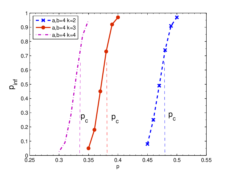
We now check the validity of these analytical results via simulations. In Figure 5, we show the variation of analytically obtained values with respect to average inter-degree for different values of . To verify these results, we pick a few sets of values , and from the curves in Figure 5 and run simulations with nodes to estimate the probability of the existence of a functional giant component in steady state. As expected [3], in all curves we see a sharp increase in as approaches a critical threshold . It is also clear from Figure 5 that, for all parameter sets, such sharp transition occurs when is close to the corresponding value given in Figure 5.
V-C A Comparison of System Robustness


In Section IV-B and IV-C, we have analytically proved that the regular allocation of bi-directional inter-edges leads to the strongest robustness against random attacks. To get a more concrete sense, we now numerically compare the system robustness of these strategies in terms of their critical thresholds . Specifically, we consider coupled Erdős-Rényi networks with mean intra-degrees and . For the sake of fair comparison, we assume that the mean inter-degree is set to for all systems; in both Systems and , the inter-degree distribution at each node is assumed to be Poisson. The critical threshold value corresponding to all three strategies are compared under a variety of conditions. For Systems and , we use the numerical results derived in Section V-A and Section V-B, respectively, while for System we use the numerical results provided in [16].
First, we compare System with System to see the difference between the proposed regular inter-edge allocation strategy and the strategy in [16]. Figure 6 depicts as a function of mean inter-degree for various values of , while Figure 6 depicts the variation of with respect to for different values. In all cases, it is seen that regular allocation of bi-directional inter-edges yields a much smaller (and thus, a more robust system) than random allocation of unidirectional inter-edges. For instance, for , System [16, Figure 2] gives , whereas, as seen via Figure 6, System yields a critical threshold at . This is a significant difference since it means that System can have a functioning giant component despite a random failure of at most of the nodes, whereas System , which uses the regular inter-edge allocation scheme proposed in this paper, is resistant to a random failure of up to of the nodes. Indeed, in some cases, our strategy can outperform that in [16] even with half the (mean) inter-degree per node. For instance, when , our strategy yields with only as compared to of the System with .
We also compare System with System in order to see the improvement in allocating bi-directional edges regularly rather than randomly. Figure 6 depicts as a function of mean inter-degree for various values of . It is seen that, in all cases, System yields a lower (and thus a more robust system) than System . For example, when and , we get for System , while for System , we find that . The difference is significant in that it corresponds to a resiliency against a random failure of up to of the nodes in System as compared to in System .
Finally, in order to better illustrate the optimality of System in terms of system robustness, we depict in Figure 6 the variation of with respect to for different values of in all three systems. It is clear that the proposed regular allocation strategy in System always yields the lowest and thus provides the best resiliency against random attacks. We also see that System always outperforms System , showing the superiority (in terms of robustness) of using bi-directional inter-edges rather than unidirectional edges.
We believe that the drastic improvement in robustness against random attacks seen in System has its roots as follows. First, in the absence of intra-topology information, it is difficult to tell which nodes play more important roles in preserving the connectivity of the networks. Thus, in order to combat random attacks, it is reasonable to treat all nodes equally and give them equal priority in inter-edge allocation. Secondly, in Systems and , there may exist a non-negligible fraction of nodes with no inter-edge support from the other network. Those nodes are automatically non-functional even if they are not attacked. But, the regular allocation scheme promises a guaranteed level of support, in terms of inter-edges, for all nodes in both networks. Finally, using bi-directional inter-edges ensures that the amount of support provided is equal to the amount of support being received for each node. Thus, the use of bi-directional inter-edges increases the regularity of the support-dependency relationship relative to unidirectional inter-edges, and this may help improve the system robustness.
VI Conclusion and Future Work
We study the robustness of a cyber-physical system in which a cyber-network overlays a physical-network. To improve network robustness against random node failures, we develop and study a regular allocation strategy that allots a fixed number of inter-network edges to each node. Our findings reveal that the proposed regular allocation strategy yields the optimal robustness amongst all strategies when no information regarding the intra-topologies of the individual networks is available. For future work, we conjecture that in the presence of such information, the topology of the networks can be exploited to further improve the robustness of cyber-physical systems against cascading failures.
It is also of interest to study models that are more realistic than the existing ones. For instance, in a realistic setting, one can expect to see a certain correlation between the inter-edges and the intra-edges of a system owing to the geographical locations of the nodes. Also, some of the nodes may be autonomous, meaning that they do not depend on nodes of the other network to function properly; in that case, one can expect the regular allocation strategy to still be the optimum if the nodes that are autonomous are not known. Clearly, there are still many open questions centered around network interdependence in cyber-physical systems. We are currently investigating related issues along this avenue.
VII Acknowledgments
We thank the anonymous reviewers for their careful reading of the original manuscript; their comments helped improve the final version of this paper. We also thank Prof. Armand Makowski for his insightful comments. Part of this material was presented in [18]. This research was supported in part by the U.S. National Science Foundation grants No. CNS-0905603, CNS-0917087, and the DTRA grant HDTRA1-09-1-0032.
References
- [1] A. L. Barabási and L. Albert, “Emergence of Scaling in Random Networks,” Science 286:509-512, 1999.
- [2] B. Bollobás, Random Graphs, Cambridge Studies in Advanced Mathematics, Cambridge University Press, Cambridge (UK), 2001.
- [3] S.V. Buldyrev, R. Parshani, G. Paul, H.E. Stanley, and S. Havlin, “Catastrophic cascade of failures in interdependent networks,” Nature, 464:1025–1028, 2010.
- [4] S. V. Buldyrev, N. W. Shere, and G. A. Cwilich, “Interdependent networks with identical degrees of mutually dependent nodes,” Physical Review E 83:016112, 2011.
- [5] D.S. Callaway, M.E.J. Newman, S.H. Strogatz, and D.J. Watts “Network robustness and fragility: Percolation on random graphs,” Physical Review Letters, 85(25):5468–5471, 2000.
- [6] W. Cho, K.I. Goh and I.M. Kim, “Correlated couplings and robustness of coupled networks,” Available online at arXiv:1010.4971v1[physics.data-an].
- [7] R. Cohen, K. Erez, D. Ben-Avraham, and S. Havlin, “Resilience of the internet to random breakdowns,” Physical Review Letters, 85(21):4626–4628, 2000.
- [8] R. Cohen and S. Havlin, Complex networks: structure, robustness and function, Cambridge University Press, United Kingdom, 2010.
- [9] CPS Steering Group, “Cyber-physical systems executive summary, 2008,” Available online at http://varma.ece.cmu.edu/summit/CPS-Executive-Summary.pdf.
- [10] X. Huang, J. Gao, S. V. Buldyrev, S. Havlin, and H. E. Stanley, “Robustness of interdependent networks under targeted attack”, Physical Review E 83: 065101, 2011.
- [11] D. E. Knuth, The Art of Computer Programming, Volume 2, Addison–Wesley, 1981.
- [12] M.E.J. Newman, “Spread of epidemic disease on networks,” Physical Review E 66(1):16128, 2002.
- [13] M.E.J. Newman, S.H. Strogatz, and D.J. Watts. “Random graphs with arbitrary degree distributions and their applications,” Physical Review E 64(2):26118, 2001.
- [14] R. Parshani, S. V. Buldyrev, and S. Havlin, “Interdependent Networks: Reducing the Coupling Strength Leads to a Change from a First to Second Order Percolation Transition,” Physical Review Letters 105:048701, 2010.
- [15] C. M. Schneider, N. A. M. Araujo, S. Havlin and H. J. Herrmann, “Towards designing robust coupled networks,” Available online at arXiv:1106.3234v1[cond-mat.stat-mech].
- [16] J. Shao, S.V. Buldyrev, S. Havlin, and H.E. Stanley, “Cascade of failures in coupled network systems with multiple support-dependent relations,” Physical Review E 83:036116, 2011.
- [17] A. Vespignani, “Complex networks: The fragility of interdependency,” Nature 464: 984-985, April 2010.
- [18] O. Yağan, D. Qian, J. Zhang, and D. Cochran, “On allocating interconnecting links against cascading failures in cyber-physical networks,” Proceedings of the Third International Workshop on Network Science for Communication Networks, (NetSciCom 2011), April 2011.
![[Uncaptioned image]](1201.2698v2/Yagan.png) |
Osman Yağan (S’07) received the B.S. degree in Electrical and Electronics Engineering from the Middle East Technical University, Ankara (Turkey) in 2007, and the Ph.D. degree in Electrical and Computer Engineering from the University of Maryland, College Park, MD in 2011. He was a visiting Postdoctoral Scholar at Arizona State University during Fall 2011. Since December 2011, he has been a Postdoctoral Research Fellow in the Cyber Security Laboratory (CyLab) at the Carnegie Mellon University. His research interests include wireless network security, dynamical processes in complex networks, percolation theory, random graphs and their applications. |
![[Uncaptioned image]](1201.2698v2/Qian.png) |
Dajun Qian received his B.S. and M.S. degrees of Electrical Engineering from Southeast University, Nanjing, China, in 2006 and 2008, respectively. Currently, he is a Ph.D. student in the Department of Electrical, Computer and Energy Engineering, Arizona State University, Tempe, AZ. His research interests include wireless communications, social networks and cyber-physical systems. |
![[Uncaptioned image]](1201.2698v2/Zhang.png) |
Junshan Zhang (S’98-M’00-F’12) received his Ph.D. degree from the School of ECE at Purdue University in 2000. He joined the EE Department at Arizona State University in August 2000, where he has been Professor since 2010. His research interests include communications networks, cyber-physical systems with applications to smart grid, stochastic modeling and analysis, and wireless communications. His current research focuses on fundamental problems in information networks and network science, including network optimization/control, smart grid, cognitive radio, and network information theory. Prof. Zhang is a fellow of the IEEE, and a recipient of the ONR Young Investigator Award in 2005 and the NSF CAREER award in 2003. He received the Outstanding Research Award from the IEEE Phoenix Section in 2003. He served as TPC co-chair for WICON 2008 and IPCCC’06, TPC vice chair for ICCCN’06, and the general chair for IEEE Communication Theory Workshop 2007. He was an Associate Editor for IEEE Transactions on Wireless Communications. He is currently an editor for the Computer Network journal and IEEE Wireless Communication Magazine. He co-authored a paper that won IEEE ICC 2008 best paper award, and one of his papers was selected as the INFOCOM 2009 Best Paper Award Runner-up. He is TPC co-chair for INFOCOM 2012. |
![[Uncaptioned image]](1201.2698v2/Cochran.png) |
Douglas Cochran (S’86-A’90-M’92-SM’96) holds M.S. and Ph.D. degrees in applied mathematics from Harvard University, Cambridge, MA, and degrees in mathematics from the Massachusetts Institute of Technology, Cambridge, and the University of California, San Diego. Since 1989, he has been on the faculty of the School of Electrical, Computer and Energy Engineering, Arizona State University (ASU), Tempe, and is also affiliated with the School of Mathematical and Statistical Sciences. Between 2005 and 2008, he served as Assistant Dean for Research in the Ira A. Fulton School of Engineering at ASU. Between 2000 and 2005, he was Program Manager for Mathematics at the Defense Advanced Research Projects Agency (DARPA) and he held a similar position in the U.S. Air Force Office of Scientific Research between 2008 and 2010. Prior to joining the ASU faculty, he was Senior Scientist at BBN Systems and Technologies, Inc., during which time he served as resident scientist at the DARPA Acoustic Research Center and the Naval Ocean Systems Center. He has been a visiting scientist at the Australian Defence Science and Technology Organisation and served as a consultant to several technology companies. Prof. Cochran was General Co-Chair of the 1999 IEEE International Conference on Acoustics, Speech and Signal Processing (ICASSP-99) and Co-Chair of the 1997 U.S.-Australia Workshop on Defense Signal Processing. He has also served as Associate Editor for book series and journals, including the IEEE TRANSACTIONS ON SIGNAL PROCESSING. His research is in applied harmonic analysis and statistical signal processing. |