Stability analysis for solitons in PT-symmetric optical lattices
Abstract
Stability of solitons in parity-time (PT)-symmetric periodic potentials (optical lattices) is analyzed in both one- and two-dimensional systems. First we show analytically that when the strength of the gain-loss component in the PT lattice rises above a certain threshold (phase-transition point), an infinite number of linear Bloch bands turn complex simultaneously. Second, we show that while stable families of solitons can exist in PT lattices, increasing the gain-loss component has an overall destabilizing effect on soliton propagation. Specifically, when the gain-loss component increases, the parameter range of stable solitons shrinks as new regions of instability appear. Thirdly, we investigate the nonlinear evolution of unstable PT solitons under perturbations, and show that the energy of perturbed solitons can grow unbounded even though the PT lattice is below the phase transition point.
pacs
42.65.Tg, 05.45.YvI Introduction
Recent interest in study of parity-time (PT) symmetric optical potentials has its roots in quantum mechanics. In quantum mechanics, in order for the energy levels to be real and the theory to be probability conserving, it is usually assumed that the Hamiltonian (Schrödinger) operator be Hermitian. However, in the past decade there has seen considerable attention [1, 2, 3, 4] in a weaker version of the Hermiticity axiom which requires that the Hamiltonian instead only exhibit space-time reflection symmetry (PT symmetry). While there has been much theoretical success in developing a non-Hermitian quantum field theory, the phenomena unique to this class of pseudo-Hermitian systems have not yet been observed experimentally.
The same Schrödinger equation from quantum mechanics applies also to optics. Motivated by this connection, optical systems which have PT-symmetric potentials have been formulated [5]. A PT-symmetric optical potential is realizable by the careful distribution of gain and loss in the media so that it satisfies the PT symmetry , where x is the spatial coordinate and ‘’ stands for complex conjugation. That is, the refractive-index profile of the media is even and gain-loss profile is odd. Such optical PT media have been created experimentally [6, 7]. These linear PT media undergo phase transition as the gain-loss component crosses a certain threshold [1, 8, 6, 7]. Below this threshold, all eigenvalues of the PT potential are real; but above this threshold, complex eigenvalues appear, hence the intensity of a light beam grows exponentially during linear propagation. The nature of this phase transition (especially for periodic PT potentials) has not been fully understood yet.
These phenomena may also be studied in a nonlinear context by considering the existence of localized modes called solitons [8, 9]. When a system contains gain and loss, solitons generally exist only at special values of the propagation constant [10]. However, since PT potentials can admit all-real linear spectra, solitons could exist at continuous ranges of the propagation constant, which is quite remarkable. So far, soliton families in PT-symmetric periodic potentials with defects and in PT-symmetric nonlinear potentials have been investigated [11, 12, 13, 14]. But stability properties of these PT solitons (especially in periodic PT potentials) have not been carefully examined.
In this paper, we investigate linear phase transition and stability of (nonlinear) solitons in PT-symmetric periodic potentials (optical lattices) in both one and two spatial dimensions. Our mathematical model is the nonlinear Schrödinger (NLS) equation with a PT lattice potential,
| (1.1) |
where denotes the focusing and defocusing nonlinearity, and the potential is periodic in and and satisfies the PT symmetry . For simplicity, we take this PT lattice potential to be
| (1.2) |
in one dimension (1D) and
| (1.3) |
in two dimensions. Here is the depth of the real component of the potential, is the relative magnitude of the imaginary component, and the period of this PT lattice is . For this system, we first show analytically that when the strength of the gain-loss component (the imaginary part of ) in the PT lattice rises above a certain threshold (phase-transition point), an infinite number of linear Bloch bands turn complex simultaneously. This simultaneous bifurcation of an infinite number of complex eigenvalues at the phase transition point has never been reported before for any PT-symmetric potentials to our best knowledge [1, 9]. Second, we show that while stable families of solitons can exist in PT lattices (below the phase transition point), increasing the gain-loss component has an overall destabilizing effect on soliton propagation. Specifically, when the gain-loss component increases, the parameter range of stable solitons shrinks as new regions of instability appear. Thirdly, we investigate the evolution of unstable PT solitons under perturbations, and show that the energy of these perturbed solitons can grow unbounded even if the PT lattice is below the phase transition point.
II Simultaneous complex-eigenvalue bifurcation at the phase transition point
We begin by investigating the bifurcation of the continuous spectrum (Bloch bands) of the linear Schrödinger operator in Eq. (1.1) at the phase transition point. The phase transition point is a point above which the spectrum is no longer purely real as the strength of the imaginary (gain-loss) contribution relative to the real (refractive-index) contribution in the potential is increased. We will show that at the phase transition point, an infinite number of Bloch bands turn complex simultaneously.
We first consider this bifurcation in one dimension. In this case, the linear Schrödinger equation is
| (2.1) |
where the PT lattice potential is given in Eq. (1.2). The continuous spectrum of this Schrödinger equation consists of Bloch modes of the form
| (2.2) |
where is a -periodic function in , is the wavenumber in the irreducible Brillouin zone , and is the propagation constant. The values of and are related. The relation is called the diffraction relation, and all admissible values of form the continuous spectrum of Eq. (2.1).
For the PT lattice (1.2), the phase transition point is known to be [8]. Below this phase transition point (), the continuous spectrum is all real and comprises an infinite number of segments (known as Bloch bands). The gaps between these Bloch bands are called bandgaps; the largest, which contains everything to the left of the continuous spectrum, is the semi-infinite gap and further gaps are numbered (in our case from left to right). As an example, at and , the diffraction relation is shown in Fig. 1 and the Bloch bands and bandgaps are shown in Fig. 2.


As increases, bandgaps shrink (see Fig. 2). At the phase transition point (), all Bloch bands merge (see Figs. 1 and 2). Above the phase transition point (), complex eigenvalues appear in the Bloch bands. This phase transition has been reported before [8]. For example, the diffraction relation at and is displayed in Fig. 1. It is seen that complex eigenvalues arise in the Bloch bands near edges of the Brillouin zone.
What was not known about this phase transition, however, is that right above this phase transition point, complex eigenvalues appear simultaneously in an infinite number of Bloch bands. To demonstrate, the dependence of eigenvalues on at Brillouin-zone edge is shown in Fig. 2. We can see that at the phase transition point , complex eigenvalues bifurcate out simultaneously from point A where the first and second Bloch bands merge, and from point C where the third and fourth Bloch bands merge, with both band-mergings occurring at the Brillouin-zone edges (this bifurcation of complex eigenvalues does not occur from point B where the second and third Bloch bands merge at the Brillouin-zone center ).
Below, we show analytically that at the phase transition point, an infinite number of complex eigenvalues bifurcate out simultaneously from an infinite number of Bloch bands. In particular, bifurcations of these complex eigenvalues occur at points where the -th and the -th Bloch bands merge (at ), but not at points where the -th and the -th Bloch bands merge (at ), for all positive integers (see Figs. 1 and 2).
We look for solutions to Eq. (2.1) of the form , where satisfies the equation
| (2.3) |
At the phase transition point , Eq. (2.3) reduces to
| (2.4) |
Under the variable transformation , this equation becomes Bessel’s equation,
| (2.5) |
thus it has exact solutions in terms of Bessel functions
| (2.6) |
where , or
| (2.7) |
This is the exact diffraction relation at the phase transition point, as can be seen by utilizing the power-series expansion of the Bessel function to expand the above Bloch solution (2.6) into a Fourier series
| (2.8) |
where is seen to be the wavenumber and is a -periodic function. By factoring out the -periodic term from (for a certain integer ) and combining it with , one can restrict the wavenumber to be in the Brillouin zone , as is customary in the Bloch theory (see Fig. 1). The diffraction relation (2.7) shows that the continuous spectrum at the phase transition point is and is entirely real. When is an integer, the two Bessel solutions in (2.6) are linearly dependent. This corresponds to the points where different Bloch bands merge (see points A, B, C, … in Fig. 2), and the associated values are
| (2.9) |
These values are located at either or of the Brillouin zone on the diffraction curves, depending on whether is even or odd (see Fig. 1), and their Bloch functions are -periodic for even and -periodic for odd .
We now consider the case where is near the phase transition point 0.5, i.e., . In this case, Eq. (2.3) becomes
| (2.10) |
whose solutions and the corresponding diffraction relation can be derived by the perturbation method. For simplicity, we only derive its solutions which are - or -periodic (these Bloch solutions are degenerate). The corresponding values are then those with or on the diffraction curves (see Fig. 1). These solutions and the associated values can be expanded as power series in ,
| (2.11a) | ||||
| (2.11b) | ||||
where , and coefficients in (2.11a) are certain constants. Details of this perturbation calculation are presented in Appendix 1. The main results for these coefficients at various values are summarized in the following table.
| 0 | 0 | 0 | |
| 1 | , | ||
| 2 | 0 | , | 0 |
| 3 | 0 | , | |
| N | 0 | 0 |
We see from this table that when , which correspond to points A, C in Fig. 2, the coefficient or is imaginary, thus complex eigenvalues bifurcate out simultaneously above the phase transition point (). In addition, the imaginary part of these complex eigenvalues at is much smaller than that at since the former is of order while the latter is of order . However, no complex eigenvalues appear when (the latter corresponds to the point B in Fig. 2). All these analytical results are in complete qualitative and quantitative agreement with Fig. 2 as we have carefully checked. Continuing these calculations to higher values, we have found that the coefficient is always imaginary for , where . Thus complex eigenvalues bifurcate out simultaneously from all odd values of at the phase transition point .
The above table also shows that below the phase transition point (, or ), the eigenvalue from the expansion (2.11a) is always real for all integers . In addition, a gap opens at the corresponding values of . Furthermore, the width of the gap is of order . Above the phase transition point, the even-numbered bandgaps reopen, whereas the odd-numbered bandgaps close and complex eigenvalues bifurcate out. All these analytical conclusions match perfectly with Fig. 2 as well.
Now we consider eigenvalue bifurcations in two dimensions. In this case, the 2D linear Schrödinger equation (1.1) is
| (2.12) |
where the PT lattice potential is given in Eq. (1.3). This 2D potential is separable, thus the Bloch modes of Eq. (2.12) are [15]
| (2.13) |
where is the 1D -periodic function as given in (2.2),
| (2.14) |
is the 2D diffraction relation, are Bloch wavenumbers in and directions and are located inside the irreducible Brillouin zone , and the function is the diffraction relation of the 1D equation (2.1). This diffraction relation (2.14) shows that complex eigenvalues appear in this 2D PT lattice if and only if complex eigenvalues appear in the 1D PT lattice (1.2). Thus all eigenvalues in the 2D system (2.12) are real when , and a phase transition occurs at above which complex eigenvalues arise. In addition, an infinite number of Bloch bands turn complex simultaneously right above this phase transition point.
III Stability of PT solitons in one dimension
In the presence of cubic nonlinearity, the mathematical model becomes the NLS equation (1.1) with a PT lattice potential. In this case, light can self-localize and form solitons. In this section, we study these PT solitons and their linear-stability behaviors in one dimension.
In one dimension, the NLS equation (1.1) becomes
| (3.1) |
Here the PT lattice is taken as (1.2) with , and . Solitons in this model are sought of the form
| (3.2) |
where is a localized function, and is a real propagation constant. These solitons can be computed by either the squared operator iteration method or the Newton-conjugate-gradient method applied to the normal equation [15]. They exist when lies inside bandgaps of the linear system for both below and above the phase transition point. Above the phase transition point (), linear waves amplify exponentially during propagation, thus any solitons would also be unstable to perturbations. So we only need to consider below.
To determine the linear stability of these PT solitons, we perturb them as
| (3.3) |
where . After substitution into equation (3.1) and linearizing, we arrive at the eigenvalue problem
| (3.4) |
where
This eigenvalue problem can be computed by the Fourier collocation method (for the full spectrum) or the Newton-conjugate-gradient method (for individual discrete eigenvalues) [15]. If eigenvalues with positive real parts exist, the soliton is linearly unstable; otherwise it is linearly stable.
We first consider PT solitons in the semi-infinite gap under focusing nonlinearity (). For , two families of PT solitons are obtained and their power curves are displayed in Fig. 3 (left). Here the power of a soliton is defined as
| (3.5) |
In this figure, the lower power curve is for the fundamental solitons which exhibit the same PT symmetry and whose real parts possess a single dominant peak. The profile of such a soliton at is displayed in Fig. 3 (right). This soliton family bifurcates out of the first Bloch band, and the solitons near this Bloch band are low-amplitude Bloch-wave packets. We have found that the entire branch of this fundamental-soliton family is linearly stable, which is indicated by solid lines of its power curve in Fig. 3 (left). The upper power curve in Fig. 3 is for the dipole solitons. This power curve features double branches which terminate before reaching the first Bloch band (a similar phenomenon occurs in purely real lattices [15, 16]). Profiles of three such solitons on the lower power branch are displayed in Fig. 4 (top). It is seen that the real parts of these dipole solitons possess two dominant peaks of opposite phase (which is why they are termed dipole solitons). Unlike the fundamental solitons, these dipole solitons are linearly stable only in a certain portion of their existence region. Specifically, only dipole solitons on the lower branch and with are stable (see Fig. 3 (left)). For dipole solitons in this region, their spectra are entirely imaginary (see Fig. 4 (bottom left)). At , stability switching occurs where a quadruple of complex eigenvalues bifurcate off of the edge of the continuous spectrum (see Fig. 4 (bottom center)). Within the unstable region, there is a second eigenvalue bifurcation at of the lower branch (near and on the left side of the power minimum) where a pair of real eigenvalues bifurcate from zero (see Fig. 4 (bottom right)). Some of these stability behaviors on dipole solitons are similar to those in the purely real potential () [15]. A notable difference is that for real potentials real eigenvalues bifurcate out of the origin exactly at the minimum of the power curve [15], whereas here this real-eigenvalue bifurcation occurs not at the power minimum. An analytical explanation for this new phenomanon will be given in Appendix 2.


Next we consider PT solitons in the first gap under defocusing nonlinearity (). Again, for , two families of PT solitons are obtained and their power curves are displayed in Fig. 5 (left) with stability results indicated. The lower curve is for fundamental solitons whose profiles at two values are depicted in Fig. 5 (top right panel), while the upper curve is for dipole solitons, whose profiles are similar to those in Fig. 6 (middle panel) below. The fundamental-soliton family bifurcates out of the first Bloch band, whereas the dipole family does not. We have found that all solitons in this dipole family are linearly unstable (see Fig. 5 (left)). The fundamental-soliton family, however, is linearly stable when . At , stability switching occurs where a pair of real eigenvalues bifurcate out from zero (see Fig. 5). Notice that unlike in real potentials [15], this zero-eigenvalue bifurcation does not occur at a power extremum since the potential here is complex. An explanation for this will be presented in Appendix 2.

The stability results of PT solitons in Figs. 3 to 5 were obtained for a specific value of 0.45. Now we discuss how these stability results change when steadily increases from 0 to 0.5. First we consider PT solitons in the semi-infinite gap under focusing nonlinearity. We find that when , the entire fundamental-soliton family remains stable. The dipole family, however, is stable only on the left side of its lower branch (see Fig. 3), and this stable region shrinks as increases. Next we consider PT solitons in the first gap under defocusing nonlinearity. When (i.e., the lattice is real), the fundamental-soliton family is stable in the entire first gap [15]. As rises above 0.3, an unstable region grows off the edge of the second band. At the stability switching point a pair of real eigenvalues bifurcate from zero as illustrated in Fig. 5. Regarding the dipole-soliton family, its entire upper branch is unstable for all values. Its entire lower branch is also unstable when . For , a certain portion of its lower branch is stable; but as increases, this stable region shrinks and then totally disappears when . To demonstrate this reduced stability of dipole solitons with increasing , the power curves of these dipole solitons at two values of 0.35 and 0.4 are shown in Fig. 6 (top panel) with stability results indicated. The soliton profiles at are also shown in the middle panel of the same figure. It is seen that the stable region of dipole solitons at is much shorter than that at . Notice also that as increases the width of the first gap decreases which is often a sign of decreased stability. The unstable region on the lower branch is largely located near the edge of the second Bloch band, and the instability in this region is caused by a quadruple of complex eigenvalues (see Fig. 6 (bottom panel)).


The above stability results of PT solitons show that as increases (but still below the phase transition point), the stable regions of PT solitons generally shrink (see Fig. 6). The only exception is the fundamental-soliton family in the semi-infinite gap under focusing nonlinearity, which remains entirely stable up to the phase transition point. Overall, the inclusion of the gain-loss component in the PT lattice has a destabilizing effect on solitons.
IV Stability of PT solitons in two dimensions
In this section we analyze the linear stability of solitons in a two-dimensional PT lattice. We will show that the destabilizing effect of the gain-loss component is more prominent in this case, even for fundamental solitons in the semi-infinite gap.
In two dimensions, the mathematical model is Eq. (1.1), or
| (4.1) |
where the PT lattice is taken as (1.3) with . Solitons in this model are sought of the form
| (4.2) |
where is a localized function, and is a real propagation constant. These solitons as well as their linear-stability spectra can be obtained by numerical methods similar to the 1D case. The phase transition point in this 2D model is also , above which all solitons are linearly unstable. Thus we only consider below.
For simplicity we only consider 2D fundamental PT solitons in the semi-infinite gap under focusing nonlinearity (). These fundamental solitons possess the PT symmetry , and their real parts have a single dominant peak. Profiles of such solitons can be found in Fig. 8 (upper panel) later. We find that these fundamental solitons are stable only on a finite -interval even for small values of . In addition, this stable region shrinks as increases and totally disappears when . To demonstrate, power curves of these solitons as well as their stability regions at two values of 0.2 and 0.3 are displayed in Fig. 7. It is seen that the stable region is finite even though the existence region of solitons is infinite. In addition, as increases from 0.2 to 0.3, the stable region has shortened by several times. For each , there are two unstable regions, one located at large negative values, and the other one located near the first Bloch band. For large negative values of the instability is due to a quadruple of complex eigenvalues, whereas for values near the first band, the instability is due to a pair of real eigenvalues. Examples of the spectrum in each region are shown in Fig. 8 with . We see that in this 2D case, even the fundamental solitons in the semi-infinite gap are destabilized by the addition of the gain-loss component in the lattice.


V Nonlinear evolution of PT solitons under perturbations
In this section, we examine the nonlinear evolution of PT solitons under weak perturbations. We find that when a PT soliton is linearly stable, then it is also nonlinearly stable and propagates robustly against perturbations. If the soliton is linearly unstable, then it breaks up under perturbations, and its amplitude and energy can grow unbounded over distance.
First we consider the 1D fundamental soliton shown in Fig. 3, which resides in the semi-infinite gap under focusing nonlinearity and is linearly stable. We perturb it by 5% random noise perturbations and then simulate its evolution in Eq. (3.1). The simulation result is shown in Fig. 9 (left). We can see that even after units of propagation, this soliton remains robust and does not break up. Thus this soliton is also nonlinearly stable. Next we consider the 1D fundamental soliton shown in Fig. 5, which resides in the first gap under defocusing nonlinearity and is linearly unstable. When this soliton is perturbed by 5% random noise perturbations, its evolution is shown in Fig. 9 (right). It is seen that this soliton quickly blows up and spreads out, thus is obviously nonlinearly unstable. Notice that the peak amplitude and energy of this perturbed soliton steadily increase without bound over distance. This indicates that the gain-loss component of the PT lattice steadily feeds energy into the solution. Recall that the value in this case is below the phase transition point, thus linear waves do not grow. Consequently the energy growth in this evolution is solely due to the nonlinear effects.

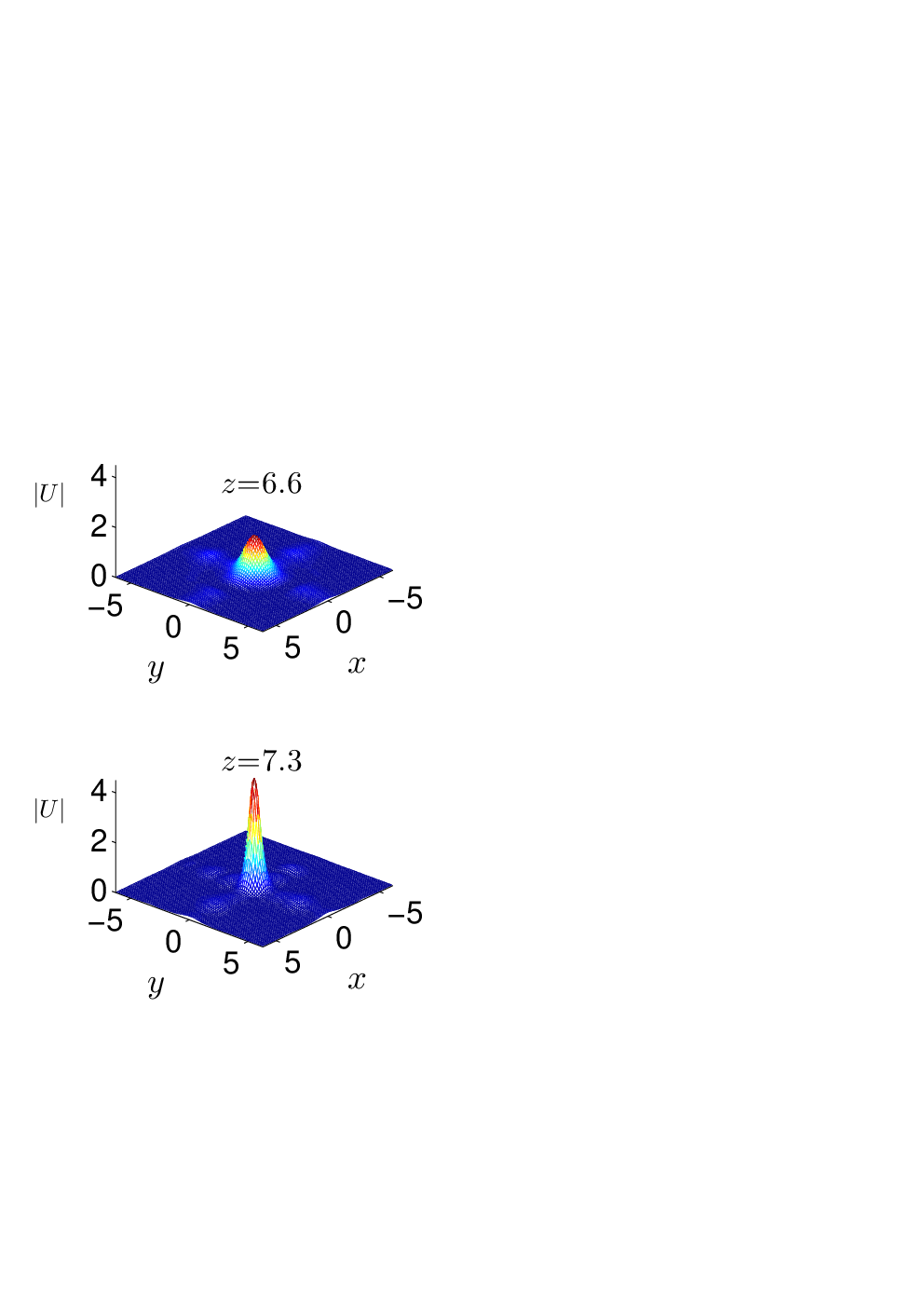
Lastly we consider the 2D fundamental soliton shown in Fig. 8 (left panel), which resides in the semi-infinite gap under focusing nonlinearity and is linearly unstable. When this soliton is perturbed by 5% random noise perturbations, its evolution is shown in Fig. 10. It is seen that the power (and peak amplitude) of this perturbed soliton also grows oscillatorily without bound, thus this soliton is nonlinearly unstable. This oscillatory growth occurs since the unstable eigenvalues of this soliton are complex (see Fig. 8 (lower left panel)).

VI Summary
In summary, we have analyzed the linear phase transition and nonlinear solitons in PT-symmetric photonic lattices. We have shown that at the phase transition point, an infinite number of linear Bloch bands turn complex simultaneously. We have also shown that while continuous ranges of stable solitons can exist in PT lattices, increasing the gain-loss component of the lattice has an overall destabilizing effect on soliton propagation. In addition, we have shown that when unstable PT solitons are perturbed, the energy of the solution can grow unbounded even though the PT lattice is below the phase transition point.
Acknowledgment
This work of S.N. and J.Y. is supported in part by the Air Force Office of Scientific Research (Grant USAF 9550-09-1-0228) and the National Science Foundation (Grant DMS-0908167). The work of L.G. is supported by a Visiting Student Scholarship from the Chinese Scholarship Council.
Appendix 1: Calculation of eigenvalue bifurcations at the phase transition point
In this appendix, we calculate eigenvalue bifurcations at the phase transition point in Eq. (2.10) by perturbation methods. The solution to this equation is required to be - or -periodic, and perturbation expansions for and eigenvalue are as given in Eq. (2.11).
Let us define the operator
| (A.1) |
After substituting expansions (2.11) into Eq. (2.10) and collecting terms of the same order in we arrive at the following system of linear equations
| (A.2a) | ||||
| (A.2b) | ||||
| (A.2c) | ||||
for . The solution is
| (A.3) |
where
| (A.4) |
and for . This solution comes directly from (2.8) by replacing the wavenumber with the integer . The remaining linear inhomogeneous equations (A.2b)-(A.2c) for will be solved by first imposing the solvability condition due to the Fredholm Alternative Theorem and then expanding the solution in terms of Fourier series.
The adjoint operator of is
| (A.5) |
and has kernel since . The Fredholm Alternative Theorem requires that the forcing terms in equations (A.2) be orthogonal to . As we have mentioned earlier, we are concerned with - and -periodic solutions here and thus define the inner product as
| (A.6) |
Using the fact that for integers , we obtain the inner product
| (A.7) |
Eq. (A.2b) for has the solvability condition
| (A.8) |
Thus, when then . For other this solvability condition is satisfied automatically and the solution may be formally written as
| (A.9) |
Expanding into Fourier series
| (A.10) |
and substituting it into we find that the coefficients satisfy the recursion relation
| (A.11) |
for all integers . The relevant coefficients are
| (A.12a) | ||||
| (A.12b) | ||||
| (A.12c) | ||||
| (A.12d) | ||||
Notice that this series also terminates in the negative direction at .
The equation (A.2c) for is
| (A.13) |
When (hence ), its solvability condition is
| (A.14) |
which gives . For , after substituting in the solution (A.9)-(A.10) for , the solvability condition of (A.13) gives
| (A.15) |
By rewriting we may again use the orthogonality of the Fourier modes to work out the inner products explicitly,
| (A.16a) | ||||||
| (A.16b) | ||||||
| (A.16c) | ||||||
Thus,
| (A.17) |
and for . This means if then is an imaginary number and, returning to the expansion for in equation (2.11a), that is a complex number for above the phase transition point, , and real below, . This is the bifurcation that occurs at edge of the Brillouin zone where the first and second bands merge (see Figs. 1 and 2).
For , we can proceed to solve Eq. (A.13) for by Fourier expansion. Then from the solvability condition for the equation we can find that
For we formally write the solution as
| (A.18) |
since we know that is well defined in view of the orthogonality (A.16b). Expanding it into a Fourier series
| (A.19) |
it is easy to find that the coefficients satisfy the recursion relation
| (A.20) |
and
Again there are only a finite number of terms in the negative direction, i.e. for .
For (hence ), Eq. (A.2c) for is
| (A.21) |
thus
| (A.22) |
and Eq. (A.2c) for is
| (A.23) |
After substituting in (A.18) for the solvability condition is
| (A.24) |
with coefficients given by
| (A.25a) | ||||
| (A.25b) | ||||
| (A.25c) | ||||
For this gives , . For we find that is a double root,
| (A.26) |
At these values, the solution is well defined and is given by
| (A.27) |
For , Eq. (A.2c) for is
| (A.28) |
After substituting in equations (A.18) and (A.22) the solvability condition for this equation reduces down to
| (A.29) |
Thus, for we must have ; and for this condition is satisfied automatically since from Eq. (A.26) is a double root of Eq. (A.24).
For , Eq. (A.2c) for is
| (A.30) |
Substituting in Eq. (A.22) and noting that (in view of (A.29)) we are left with the solvability condition
| (A.31) |
This condition may be further simplified,
Thus for , we get
| (A.32) |
and for , we get . This shows that there is another bifurcation point of complex eigenvalues at , where the third bandgap closes (see Figs. 1 and 2).
The results of the above perturbation calculations are summarized in Table 1 of the main text. Continuing these calculations to higher values, we have found that the coefficient is always imaginary for , where . Thus complex eigenvalues bifurcate out simultaneously from at the phase transition point .
Appendix 2: Analytical criterion for zero-eigenvalue bifurcation of solitons in complex potentials
In real potentials (such as when in (1.2)), the power curve does more than just a convenient way to catalogue and parameterize a continuous family of solitons for various values of the propagation constant . Specifically, whenever the power curve has a local extremum the zero eigenvalue in the linear-stability spectrum of solitons then bifurcates out along the real and imaginary axes on the two sides of the power extremum respectively, leading to a change of stability at the power extremum (if no other unstable eigenvalues exist) [15]. In this appendix we consider the extension of this concept to general complex potentials (which include PT-symmetric lattices as special cases). The resulting analytical criterion for zero-eigenvalue bifurcation will explain the stability switchings in Fig. 5 and Fig. 7 (right side), as well as the onset of real eigenvalues in Fig. 4 (right panel).
Let us begin with the eigenvalue problem (3.4) derived in the main text,
| (A.33) |
where we know that is always an eigenvalue with algebraic multiplicity of at least two due to phase invariance of Eq. (1.1). The eigenfunction and generalized eigenfunction of this zero eigenvalue associated with the phase invariance can be written explicitly in terms of the soliton ,
Thus, for nonzero eigenvalues to bifurcate out from the origin, must have algebraic multiplicity of at least 3 at that point. A sufficient condition for this to occur is that there be a second generalized eigenfunction which solves
| (A.34) |
We now use the Fredholm Alternative Theorem to derive the solvability condition for Eq. (A.34). Let us denote the kernel of the adjoint operator as , i.e.,
| (A.35) |
where the adjoint operator is
| (A.36) |
Here the superscript “” stands for transpose of a matrix. Then the solvability condition of Eq. (A.34) is
| (A.37) |
which is a sufficient condition (criterion) for zero-eigenvalue bifurcation in general complex potentials.
For real potentials, it is easy to see that
| (A.38) |
thus the above criterion reduces to , i.e., the extremum of the power curve [15]. For general complex potentials, however, is not equal to the above expression, thus stability switching will no longer occur at a power extremum. An example of this has been seen in Fig. 5.
References
- [1] C.M. Bender and S. Boettcher, “Real spectra in non-Hermitian Hamiltonians having PT symmetry”, Phys. Rev. Lett. 80, 5243-5246 (1998).
- [2] C.M. Bender, D.C. Brody, and H.F. Jones, “Complex extension of quantum mechanics,” Phys. Rev. Lett. 89, 270401 (2002).
- [3] Z. Ahmed, “Real and complex discrete eigenvalues in an exactly solvable one-dimensional complex PT-invariant potential”, Phys. Lett. A 282, 343-348 (2001).
- [4] A. Mostafazadeh, “Exact PT-symmetry is equivalent to Hermiticity”, J. Phys. A: Math. Gen. 36, 7081-7091 (2003).
- [5] R. El-Ganainy, K.G. Makris, D.N. Christodoulides, and Z.H. Musslimani, “Theory of coupled optical PT-symmetric structures,” Opt. Lett. 32, 2632-2634 (2007).
- [6] A. Guo, G.J. Salamo, D. Duchesne, R. Morandotti, M. Volatier-Ravat, V. Aimez, G.A. Siviloglou, and D.N. Christodoulides, “Observation of PT-Symmetry Breaking in Complex Optical Potentials”, Phys. Rev. Lett. 103, 093902 (2009).
- [7] C.E. Rueter, K.G. Makris, R. El-Ganainy, D.N. Christodoulides, M. Segev, and D. Kip, “Observation of parity-time symmetry in optics”, Nature Phys. 6, 192-195 (2010).
- [8] Z.H. Musslimani, K.G. Makris, R. El-Ganainy, and D.N. Christodoulides, “Optical solitons in PT periodic potentials”, Phys. Rev. Lett. 100, 030402 (2008).
- [9] K.G. Makris, R. El-Ganainy, D.N. Christodoulides, and Z.H. Musslimani, “PT-symmetric periodic optical potentials”, Int. J. Theor. Phys. 50, 1019-1041 (2011).
- [10] N. Akhmediev and A. Ankiewicz (Editors), Dissipative Solitons (Springer, Berlin, 2005).
- [11] H. Wang and J. Wang, “Defect solitons in parity-time periodic potentials”, Opt. Express 19, 4030-4035 (2011).
- [12] Z. Lu and Z. Zhang, “Defect solitons in parity-time symmetric superlattices”, Opt. Express 19, 11457-11462 (2011).
- [13] F.K. Abdullaev, Y.V. Kartashov, V.V. Konotop, and D.A. Zezyulin, “Solitons in PT-symmetric nonlinear lattices”, Phys. Rev. A 83, 041805 (2011).
- [14] D.A. Zezyulin, Y.V. Kartashov, and V.V. Konoto, “Stability of localized modes in PT -symmetric nonlinear potentials”, http://arxiv.org/abs/1111.0898v1, 2011.
- [15] J. Yang, Nonlinear Waves in Integrable and Nonintegrable Systems (SIAM, Philadelphia, 2010).
- [16] T.R. Akylas, G. Hwang and J. Yang, “From nonlocal gap solitary waves to bound states in periodic media”, Proc. Roy. Soc. A 468, 116-135 (2012).