Restricted numerical shadow and geometry of quantum entanglement

Elements of a Hilbert space are used as basic objects of the quantum theory. A physical system with $D$ distinguishable states can be described by an element $|\psi\rangle$ of the complex Hilbert space ${\cal H}_{D}$. It is assumed that such a pure quantum state is normalized, $||\psi||^{2}=\langle\psi|\psi\rangle=1$, so it belongs to the hypersphere of dimension $2D-1$. One identifies any two states, which differ only by a global phase, $|\psi\rangle\sim|\phi\rangle=e^{\mathrm{i}\alpha}|\psi\rangle$. The set of all pure quantum states $\Omega_{D}$ acting on ${\cal H}_{D}$ is therefore equivalent to the complex projective space, $\Omega_{D}={\mathbbm{C}}\mathbf{P}^{D-1}$ (see e.g. [8]).

Any convex combination of projectors onto pure states forms a mixed quantum state, $\rho=\sum_{i}p_{i}|\psi_{i}\rangle\langle\psi_{i}|$ with $p_{i}\geq 0$ and $\sum_{i}p_{i}=1$. Any such state $\rho$, also called a density operator, is Hermitian, positive and normalized by the trace condition, Tr$\rho=1$. Thus the set ${\cal Q}_{D}$ of all density matrices of order $D$ forms a convex set of $D^{2}-1$ real dimensions. The projectors corresponding to the extremal points of the set of density operators form the set of pure quantum states, $\Omega_{D}={\mathbbm{C}}\mathbf{P}^{D-1}\subset{\cal Q}_{D}$. In the one qubit case, $D=2$, the set of pure quantum states forms the Bloch sphere, $\Omega_{2}={\mathbbm{C}}\mathbf{P}^{1}$, which in this case is equivalent to the boundary of the Bloch ball ${\cal Q}_{2}$. For a larger dimension the $(2D-2)$–dimensional set of pure states $\Omega_{D}$ forms only a zero–measure subset of the $D^{2}-2$ dimensional boundary of the set ${\cal Q}_{D}$.

Note that the definitions of the set of pure and mixed quantum states are unitarily invariant, so they can be formulated without specifying any basis in the Hilbert space. On the other hand, among quantum states, one distinguishes also the set of classical states, which are formed by the density matrices diagonal in a certain basis. Hence any classical state $p$ is represented by a normalized probability vector, $p=\{x_{1},x_{2},\dots,x_{D}\}$ such that $x_{i}\geq 0$ and $\sum_{i=1}^{D}x_{i}=1$. The set of classical states forms thus the probability simplex $\Delta_{D-1}\subset{\mathbbm{R}}^{D-1}$. Each of $D$ corners of the simplex represents a classical pure state, and their convex hull is equivalent to $\Delta_{D-1}$. In the one qubit case, $D=2$, the set $\Delta_{1}$ of classical states forms an interval which joins two poles of the Bloch sphere and traverses across the interior of the Bloch ball of one–qubit mixed quantum states.

The definition (1) of the numerical range of a matrix $A$ of order $D$ specifies $W(A)$ as the set of expectation values $\langle\psi|A|\psi\rangle$ for normalized pure states $|\psi\rangle$. In fact the compact set $W(A)$ in the complex plane can be considered as a projection of the set ${\cal Q}_{D}$ of quantum states onto a two plane. The following facts were recently established in [28].

Thus by fixing the dimension $D$ and selecting various operators $A$ of this order and analysing their numerical ranges $W(A)$ we may gather information about the projections of the set of quantum states. For instance, for $D=2$ the projections of the Bloch sphere form ellipses (which could form circles or may reduce an intervals), and so the numerical range of any operator $A$ of size $D=2$ may be the result. Similarly the numerical range of operators of size $D=3$ can be viewed as projections of the set $\Omega_{3}={\mathbbm{C}}\mathbf{P}^{2}$ of single qutrit quantum states, while the numerical range for matrices of order $D=4$ can be associated with projections of the set $\Omega_{4}={\mathbbm{C}}\mathbf{P}^{3}$ [26, 28].

The Haar measure on the unitary group $\mathrm{U}(D)$ induces on the set $\Omega_{D}$ of quantum pure states the unitarily invariant Fubini-Study measure $\mu$. In the simplest case of $D=2$ this measure corresponds to the uniform distribution of points on the Bloch sphere $\Omega_{2}=\mathbf{S}^{2}$.

For any operator $A$ of size $D$ we may compute its expectation value for random pure state $|\psi\rangle\in\Omega_{D}$ chosen with respect to measure $\mu$. In this way for any operator $A$ we define its numerical shadow – a probability distribution (3) on the complex plane. Note that by construction the numerical shadow $P_{A}(z)$ is supported on the numerical range $W(A)$. Furthermore, the numerical shadow is unitarily invariant: $P_{A}(z)=P_{UAU^{\dagger}}(z)$.

For any normal matrix $A$, which commutes with its adjoint, the numerical shadow $P_{A}(z)$ covers the numerical range $W(A)$ with the probability corresponding to a projection of a regular simplex $\Delta_{D-1}$ of classical states embedded in ${\mathbbm{R}}^{D-1}$) onto a plane. In general, for a non–normal operator $A$ acting on ${\cal H}_{D}$, its shadow covers the numerical range $W(A)$ with the probability corresponding to an orthogonal projection of the complex projective manifold $\Omega_{D}={\mathbbm{C}}\mathbf{P}^{D-1}$ onto a plane.

In this work we will analyse the numerical range restricted [21] to a certain subsets $R$ of pure quantum states and the corresponding restricted numerical shadows, with probability density determined by random states distributed on the subset $R$ according to the measure induced by the Fubini–Study measure on $\Omega_{D}$.

Consider a diagonal matrix of size $D$, namely $X={\rm diag}(x_{1},\dots x_{D})$. Let $|1\rangle$ be an arbitrary fixed pure state in ${\cal H}_{D}$. Then the entire set of random pure states can be obtained as $|\psi\rangle=U|1\rangle$, where $U\in\mathrm{U}(D)$ is a random unitary matrix distributed according the Haar measure. Thus the expansion coefficients of the state $|\psi\rangle$ read $(U_{11},U_{12},\dots,U_{1D})$.

The numerical shadow of the operator $X$ is defined as the density distribution of random numbers $z:=\langle\psi|X|\psi\rangle$, where $|\psi\rangle$ is a random state defined by the random unitary matrix $U$. Therefore

Note that the vector of coefficients $q={q_{1},\dots q_{D}}$ with $q_{i}=|U_{ij}|^{2}$ belongs to the $D-1$ dimensional simplex $\Delta_{D-1}$. So the complex random variable $z$ can be treated as a scalar product, $z=x\cdot q$ where the complex vector $x$ is given by the diagonal of the operator $X$, while the probability vector $q$ is random. Its distribution inside the simplex depends on the distribution in the space of unitary matrices $\mathrm{U}(D)$. In cases of interest for us this distribution belongs to the class of Dirichlet distributions parametrized by a real number $s$,

In particular, we are interested in two situations.

• A)

  Standard (complex) numerical shadow [26, 28], generated by the Haar measure on $\mathrm{U}(D)$. Then the vector $q$ is distributed uniformly with respect to the flat (Lebesgue) measure on $\Delta_{D-1}$, i.e. the Dirichlet measure with the Dirichlet parameter $s=1$ [8].

• B)

  Real numerical shadow, generated by the Haar measure on the group $\mathrm{O}(N)$ of orthogonal matrices. Then the vector $p$ is distributed with respect to the statistical measure, $P_{1/2}(q)\propto 1/\sqrt{q_{1}\cdots q_{D}}$, i.e. the Dirichlet measure with the Dirichlet parameter $s=1/2$.

In both cases the shadow covers the entire numerical range of $X$, equal to the convex hull of the spectrum $\{x_{i}\}_{i=1}^{D}$ with a density determined by the appropriate Dirichlet distribution. The case of real numerical shadow, i.e. the shadow with respect to the real pure states is treated in more detail in the subsequent section.

Consider the subset of pure quantum states of size $D$, that can be represented by real expansion coefficients in a given basis. This set forms a $(D-1)$ dimensional real projective space ${\mathbbm{R}}\mathbf{P}^{D-1}\subset{\mathbbm{C}}\mathbf{P}^{D-1}$.

Substituting into the definition (2) of a restricted numerical range [19, 21] the set ${\mathbbm{R}}\mathbf{P}^{D-1}\subset{\mathbbm{C}}\mathbf{P}^{D-1}$ as the subset $R$ of $\Omega_{D}$ we arrive at the numerical range restricted to real states. In general the restricted numerical range needs not to be convex or simply connected. Similarly, restricting the integration in (4) to the set ${\mathbbm{R}}\mathbf{P}^{D-1}$ of real quantum states we obtain the shadow of the operator $A$ with respect to real states. For brevity we will also use a shorter expression, the real shadow of $A$.

In the case of $D=2$ the set of real states forms the real projective space equivalent to a circle, ${\mathbbm{R}}\mathbf{P}^{1}\sim\mathbf{S}^{1}$. Thus the real shadow of a generic, non-normal matrix of size two forms a singular probability distribution supported on an elliptic curve in the complex plane, and not inside its interior.

The real shadows presented in Fig. 1 are obtained for illustrative operators of size $D=2$

$D=3$,

and $D=4$

These probability distributions can be thus interpreted as shadows of real projective spaces ${\mathbbm{R}}\mathbf{P}^{2}$, ${\mathbbm{R}}\mathbf{P}^{3}$ and ${\mathbbm{R}}\mathbf{P}^{4}$ on a plane. In the case 1(b) and 1(d) the shadow is supported on a real line, so we plot the corresponding probability distribution $P_{A}^{\mathbbm{R}}(x)$. In the other cases 1(a), 1(c) and 1(e) the real shadow is supported on the complex plane, so the density is encoded in the grey scale. The circle drawn by red dotted line represents the image of the sphere of dimension $D^{2}-1$, in which the set of quantum states can be inscribed. The blue dotted line represents the boundary of the standard numerical range of an operator. The restricted shadow is supported in this set or its subset.

The numerical shadow carries also some information about the higher rank numerical range [30, 31] of an operator. For instance, the darker area of the shadow corresponding to a larger probability [28] allows one to recognize in Fig. 2 the numerical range of rank $2$, written $\Lambda_{2}(U)$ of selected unitary matrices. In the case of $D=4$ shown in Fig. 2 2(a) it is equal to a single point at which the two diagonals of the quadrangle cross, while for the case $D=5$ shown in panel 2(b) the numerical range of rank two is represented by the inner pentagon located inside the numerical range in this case numerical shadow appears to be uniform in the set $\Lambda_{2}(U_{5})$. In the case $D=7$ shown in the panel 2(c) one can see darker areas between segments connecting every other eigenvalue.

Given $M\in M_{N}(\mathbb{C})$, the real shadow is taken to mean the distribution of $(Mx,x)$ when $x\in\mathbb{R}^{N}$ is a unit vector randomly chosen from the uniform distribution on $S^{N-1}=\{x\in\mathbb{R}^{N}:\|x\|=1\}$.

If $M$ itself is real, we have $(Mx,x)=(x,Mx)$ so that the distribution of $(Mx,x)$ is the same as that of the symmetric $(M+M^{T})/2$. Since the uniform distribution on $S^{N-1}$ is invariant under orthogonal transformations, we are free to diagonalize this symmetric matrix. In other words, the real shadow of $M\in M_{N}(\mathbb{R})$ is that of $\mathrm{diag}(a_{1},\dots,a_{N})$, where $a_{k}$ are the (real) eigenvalues of $(M+M^{T})/2$. Thus we need the distribution of

It is known that $x$ uniform on $S^{N-1}$ implies that $p=(x_{1}^{2},\dots,x_{n}^{2})$ has a Dirichlet–(1/2) distribution on the simplex $\Delta_{N-1}=\{p\in[0,1]^{N}:\sum_{1}^{N}p_{k}=1\}$, ie. its density is proportional to $1/\sqrt{p_{1}p_{2}\dots p_{N}}$.

The distribution of (10) is known in general [36], so for $a_{N}<a_{N-1}<\dots<a_{1}$ we have

As an example, let us consider the Jordan nilpotent $J_{3}=\left(\begin{smallmatrix}0&1&0\\ 0&0&1\\ 0&0&0\end{smallmatrix}\right).$ For the real shadow of $J_{3}$, we first note that it is the same as that of $\mathrm{diag}(1/\sqrt{2},0,-1/\sqrt{2})$. Rescaling for convenience, we compute the real shadow of $\mathrm{diag}(1,0,-1)$. The density $g_{3}(t)$ of $p_{1}-p_{3}$ is 0 outside $[-1,1]$, satisfies $g_{3}(-t)=g_{3}(t)$, and, in view of the Dirichlet–(1/2) distribution on $\Delta_{2}$, $g_{3}(t)$ is proportional to

for $0<t<1$. In particular, $g_{3}(0)=+\infty$. In [36] the case $N=3$ is treated in terms of hypergeometric functions and we can compute

for $t\in(0,1)$.

For a general $M\in M_{N}(\mathbb{C})$, one may write $M=A+\mathrm{i}B$ with $A,B\in M_{N}(\mathbb{R})$, and by diagonalizing $(A+A^{T})/2$ and $(B+B^{T})/2$ we may understand the distributions of $(Ax,x)$ and $(Bx,x)$ separately, using the techniques above. Usually the joint distribution will be obscure, but we may have some hope of understanding it in certain cases. If, for example, $M$ is normal and presented in diagonal form, it may be possible to see how the horizontal and vertical distributions knit together.

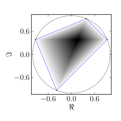
Fig. 3 shows various shadows of $M$ when $M$ is a $4\times 4$ unitary (in diagonal form). The sort of 1D shadow density seen in the left panel of Fig. 3(a) seems typical; notably, the real density of a $4\times 4$ Hermitian is constant between the two middle eigenvalues. Presumably, the vertical density has a similar form. Fig. 4 presents two examples of real shadow of generic unitary matrices of dimension five. Support of the shadow does not coincide with numerical range of those matrices because a generic unitary matrix can not be diagonalized using only orthogonal matrices.

Since methods based on moments of the shadow distribution were so effective in the complex case, we may try to mimic them for the real shadow. It is not hard to adapt the method outlined at the beginning of the proof of Proposition 5.1 from [26] to show that, for $\alpha\in\mathbb{N}_{0}^{N}$

unless each component of $\alpha$ is even, and that

Here we use the shifted factorial notation: $(x)_{n}=x(x+1)\dots(x+n-1)$, with the convention $(x)_{0}=1$; also $|\beta|$ denotes $\sum_{1}^{N}\beta_{k}$.

In principle, we can use Eq. (14) to evaluate the moments of the real shadow density $g(t)$ of $\mathrm{diag}(a_{1},\dots,a_{N})$

In the complex case we were able to progress beyond this point, obtaining such effective relations for the moments as the determinant relation (see: Eq. (10) in [26]).

As a test case, we may try to use Eq. (15) to find the moments of $g_{3}(t)$, the real shadow density of $\mathrm{diag}(1,0,-1)$, discussed in the previous example. We have

and finally we obtain that

It can be shown, that for even $n=2m$ we have

To see this we start with equation Eq. (16). Changing the index of summation from $k$ to $n-k$ shows that the sum equals $\left(-1\right)^{n}$ times itself, hence equals zero for odd $n$. Now suppose that $n=2m,m=0,1,2,\ldots$. The sum can be written in hypergeometric form

Kummer’s summation formula (see [38, p. 10]) implies (later we set $a=-2m,b=\frac{1}{2}$)

Now we set $a=-2m$ and use the terminating form of Gauss’s sum (the Chu-Vandermonde formula) to obtain

Thus, setting $b=\frac{1}{2}$ we obtain, that the integral equals

We use the variance of a complex random variable to give quantitative insight into Figs. 2-4. The calculations leading to the following formulae are based on the values of integrals of monomials over the real or complex unit spheres. Suppose $A$ is a normal matrix, written in the form $A=VDV^{{\dagger}}$ where $V$ is unitary and $D$ is diagonal with entries $\lambda_{1},\lambda_{2},\ldots,\lambda_{N}$. Thus the columns of $V$ are eigenvectors of $A$. Let $X$ denote the random variable $\left\langle\psi|A|\psi\right\rangle$ and let $m=\frac{1}{N}trA=\frac{1}{N}\sum_{j=1}^{N}\lambda_{j}$. If $\psi$ is a random vector in the unit sphere in $\mathbb{R}^{N}$ or $\mathbb{C}^{N}$ then $\mathcal{E}X=m$ (where $\mathcal{E}$ denotes the expectation). Denote the complex variance $v\left(X\right)=\mathcal{E}\left(\left|X-m\right|^{2}\right)$, a measure of (2-dimensional) spread of $X$. For the complex shadow one finds

For the real shadow and when $A$ can be diagonalized by a real orthogonal matrix, that is, $V$ is orthogonal ($VV^{T}=I$) then

which is larger than the variance of the complex shadow (see Fig. 3(b) ). In the general real case $V$ is not orthogonal, then set $C\left(V\right)_{ij}=\left|\sum_{k=1}^{N}V_{ki}V_{kj}\right|^{2}$ for $1\leq i,j\leq N$. Thus $C\left(V\right)$ is a symmetric unistochastic matrix, and its eigenvalues all lie in $\left[-1,1\right]$. By straightforward computations we find

a positive quadratic form in $\left(\lambda_{i}-m\right)_{i=1}^{N}$. The eigenvalues of $I+C\left(V\right)$ lie in $\left[0,2\right]$, and all equal $2$ when $V$ is real orthogonal.

As example consider the unitary Fourier matrix whose entries are primitive $N^{th}$ roots of unity : $V_{jk}=\frac{1}{\sqrt{N}}\exp\left(\frac{2\pi i}{N}\left(j-1\right)\left(k-1\right)\right),1\leq j,k\leq N$. Then $C\left(V\right)_{jk}=1$ if $j+k\equiv 2\operatorname{mod}N$ otherwise $C\left(V\right)_{jk}=0$. The eigenvalues of $I+C\left(V\right)$ are $2$ with multiplicity $\left\lfloor\frac{N}{2}\right\rfloor+1$ and $0$ with multiplicity $\left\lfloor\frac{N-1}{2}\right\rfloor$. The matrix $C\left(V\right)$ also contains information about approximating the eigenvectors of $A$ by points on $S^{N-1}$: indeed $\min\left\{\sum_{j=1}^{N}\left|\psi_{j}-cV_{jk}\right|^{2}:\left|c\right|=1,\psi\in S^{N-1}\right\}=2-\sqrt{2\left(1+C\left(V\right)_{kk}^{1/2}\right)}$. In particular if some $\lambda_{k}$ is an extreme point in the convex hull of $\left\{\lambda_{j}:1\leq j\leq N\right\}$ then $\lambda_{k}$ is in the real numerical range of $A$ if and only if $\left|\sum_{j=1}^{N}V_{jk}^{2}\right|=1$. This is illustrated by Fig. 4.

In the case of separable shadow of matrix $X\in\mathcal{M}_{N^{2}}$ it is possible to obtain explicit expressions for the mean and the variance. We have

and

Formulas involve the partial traces ${\rm tr}_{A}X$ and ${\rm tr}_{B}X$, follows from more general fact given in Appendix B. These expressions imply directly the following result.

Consider a diagonal matrix $X$ defined on a composite Hilbert space, ${\cal H}_{D}={\cal H}_{N}\otimes{\cal H}_{M}$ of dimension $D=NM$. Its diagonal elements forming the spectrum $\{x_{i}\}_{i=1}^{D}$ can be also represented by two indices, $\{y_{\mu\nu}\}$ with $\mu=1,\dots,N$ and $\nu=1,\dots,M$.

Let $|1,1\rangle$ be an arbitrary fixed pure product state in ${\cal H}_{D}$, so the set of random separable pure states can be obtained as $|\psi\rangle=U|1,1\rangle=W\otimes V|1,1\rangle$, where $W\in\mathrm{U}(N)$ and $V\in\mathrm{U}(M)$ are independent random unitary matrices distributed according to the Haar measure. Thus the expansion coefficients of the product state $|\psi\rangle$ read $(U_{11},U_{12},\dots,U_{1D})=(W_{11}V_{11},\dots,W_{1N}V_{1M})$.

The separable numerical shadow of the diagonal operator $X$ is defined as the density distribution of random numbers $z:=\langle\psi|X|\psi\rangle$, where $|\psi\rangle$ is a separable random state defined by random unitaries $U$ and $V$. In this case one has

where $r$ is a real probability vector of size $D=NM$. It can be considered as a tensor product of two probability vectors $p\in\Delta_{N-1}$ and $q\in\Delta_{M-1}$, since its components read $r_{\mu\nu}=p_{\mu}q_{\nu}$ with with $\mu=1,\dots N$ and $\nu=1,\dots,M$.

Thus the separable numerical shadow of a diagonal operator can be considered as a projection of the Cartesian product of classical probability simplices, $\Delta_{N-1}\times\Delta_{M-1}$. In the simplest case of $D=4=2\times 2$ the Cartesian product of two intervals (1-simplices) forms a square, which lives inside the tetrahedron of the $4$–dimensional probability vectors.

As in the previous case we can distinguish two probability measures in the space of unitary matrices. They lead to

• C)

  complex separable shadow, generated by the Haar measure on $\mathrm{U}(N)$ and $\mathrm{U}(M)$, for which both probability vectors $p$ and $q$ are distributed uniformly with respect to the Lebesgue measure on the simplices $\Delta_{N-1}$ and $\Delta_{M-1}$, respectively.

• D)

  Real separable shadow, generated by the Haar measure on the orthogonal groups $\mathrm{O}(N)$ and $\mathrm{O}(M)$, which lead to the statistical measure (Dirichlet measure with $s=1/2$) in both simplices.

Note that in these case the separable shadow of $X$ is supported on its product numerical range [21], which in general forms a proper subset of the convex hull of the spectrum. The product structure of the classical probability vector $r$ in (24), generalized for a multiple tensor product structure, is consistent with the parametrization of the product numerical range described in Prop. 12 in [21].

References

- [1] R. Horodecki, P. Horodecki, M. Horodecki, K. Horodecki, Quantum entanglement, Rev. Mod. Phys. 81, 865-942 (2009).
- [2] M. Kuś and K. Życzkowski, Geometry of entangled states, Phys. Rev. A 63, 032307-13 (2001)
- [3] R. Mosseri, R. Dandoloff, Geometry of entangled states, Bloch spheres and Hopf fibrations, J. Phys. A34, 10243 (2001). 2001 J. Phys. A: Math. Gen. 34 10243
- [4] F. Verstraete, J. Dehaene, B. De Moor, On the geometry of entangled states, J. Mod. Opt. 49, 1277 (2002)
- [5] P. Levay, The geometry of entanglement: metrics, connections and the geometric phase, J. Phys. A37, 1821-1842 (2004).
- [6] J. E. Avron, O. Kenneth, Entanglement and the geometry of two qubit, Ann. Phys. (N.Y.) 324, 470-496 (2009).
- [7] R. Bertlmann, P. Krammer, Entanglement witnesses and geometry of entanglement of two–qutrit states, Ann. Phys. (N.Y.) 324, 1388-1407 (2009)
- [8] I. Bengtsson and K. Życzkowski, Geometry of Quantum States, Cambridge University Press, 2006.
- [9] D. C. Brody, A. C. T. Gustavsson, L. P. Hughston, Entanglement of three-qubit geometry, J. Physics: Conf. Ser. 67, 012044 (2007).
- [10] A. Sawicki, A. Huckleberry, M. Kuś, Symplectic geometry of entanglement, Commun. Math. Phys. 305,441-468 (2011)
- [11] V. Vedral, Introduction to Quantum Information Science, Oxford University Press, Oxford 2007
- [12] D. Petz, Quantum Information Theory and Quantum Statistics, Springer, 2008.
- [13] M. Sinołȩcka, K. Życzkowski and M. Kuś, Manifolds of equal entanglement for composite quantum systems, Acta Phys. Pol. B 33, 2081-2095 (2002).
- [14] R. A. Horn and C. R. Johnson. Topics in Matrix Analysis. Cambridge University Press, Cambridge, U.K., 1994.
- [15] K. E. Gustafson and D. K. M. Rao. Numerical Range: The Field of Values of Linear Operators and Matrices. Springer-Verlag, New York, 1997.
- [16] E. Gutkin, The Toeplitz-Hausdorff theorem revisited: relating linear algebra and geometry Math. Intelligencer 26, 8-14 (2004).
- [17] E. Jonckheere, F. Ahmad, E. Gutkin, Differential topology of numerical range Lin. Alg. Appl. 279 227–254 (1998).
- [18] D. Henrion Semidefinite geometry of the numerical range E.J. Lin. Alg. 20 322-332 (2010).
- [19] T. Schulte-Herbrüggen, G. Dirr, U. Helmke, and S. J. Glaser. The significance of the -numerical range and the local c-numerical range in quantum control and quantum information, Linear and Multilinear Algebra 56, 3-26 (2008)
- [20] D. W. Kribs, A. Pasieka, M. Laforest, C. Ryan, and M. P. Silva. Research problems on numerical ranges in quantum computing. Linear and Multilinear Algebra 57, 491-502 (2009).
- [21] P. Gawron, Z. Puchała, J. A. Miszczak, Ł. Skowronek, M.-D. Choi, and K. Życzkowski, Restricted numerical range: a versatile tool in the theory of quantum information, J. Math. Phys. 51 102204 (24pp) (2010).
- [22] M. Marcus and B. Wang. Some variations on the numerical range. Linear and Multilinear Algebra, 9:111–120, 1980.
- [23] N. Bebiano, C. K. Li, and J. da Providencia. The numerical range and decomposable numerical range of matrices. Linear and Multilinear Algebra, 29:195–205, 1991.
- [24] G. Dirr, U. Helmke, M. Kleinsteuber, and T. Schulte-Herbrüggen. Relative c-numerical ranges for applications in quantum control and quantum information. Linear and Multilinear Algebra 56, 27-51 (2008).
- [25] Z. Puchała, P. Gawron, J.A. Miszczak, Ł. Skowronek, M.-D. Choi, K. Życzkowski, Product numerical range in a space with tensor product structure, Linear Algebra Applications 434, 327-342 (2010).
- [26] C.F. Dunkl, P. Gawron, J.A. Holbrook, Z. Puchała and K. Życzkowski, Numerical shadows: Measures and densities on the numerical range, Lin. Algebra Appl 434, 2042-2080 (2011).
- [27] T. Gallay and D. Serre, The numerical measure of a complex matrix, preprint arXiv:1009.1522
- [28] C.F. Dunkl, P. Gawron, J.A. Holbrook, J. Miszczak, Z. Puchała and K. Życzkowski, Numerical shadow and geometry of quantum states, J. Phys. A: Math. Theor., Vol. 44, No. 33 (2011), p. 335301 preprint arXiv:1104.2760
- [29] C. M. Caves, C. A. Fuchs and P. Rungta, Entanglement of formation of an arbitrary state of two rebits, Found. Phys. Lett. 14, 199-212 (2001)
- [30] M.-D. Choi, D. W. Kribs, and K. Życzkowski, Higher-Rank Numerical Ranges and Compression Problems, Lin. Alg. Appl. 418, 828-839 (2006).
- [31] M.-D. Choi, J. A. Holbrook, D. W. Kribs, and K. Życzkowski, Higher-rank numerical ranges of unitary and normal matrices, Operators and Matrices 1, 409-426 (2007).
- [32] I. Bengtsson, A. Ericsson, M. Kuś, W. Tadej, and K. Życzkowski, Birkhoff’s polytope and unistochastic matrices, and , Comm. Math. Phys. 259, 307-324 (2005).
- [33] C. Dunkl and K. Życzkowski, Volume of the set of unistochastic matrices of order 3 and the mean Jarlskog invariant, J. Math. Phys. 50, 123521 (2009).
- [34] B. Collins and P. Śniady, Integration with respect to the Haar measure on unitary, orthogonal and symplectic group, Commun. Math. Phys. 264, 773–795 (2006).
- [35] W. Dür, G. Vidal, J.I Cirac, Three qubits can be entangled in two inequivalent ways, Phys. Rev. A 62, 062314 (2000).
- [36] S. B. Provost and Y. H. Cheong, On the distribution of linear combinations of the components of a Dirichlet random vector, Canadian Journal of Statistics 28, 417–425 (2000).
- [37] Z. Puchała, J.A. Miszczak, Symbolic integration with respect to the Haar measure on the unitary group in Mathematica, preprint: arXiv:1109.4244.
- [38] W.N. Bailey, Generalized Hypergeometric Series, Cambridge University Press, 1935.
- [39] C. F. Dunkl, Intertwining operators associated to the group , Trans. Amer. Math. Soc. 347 (1995), 3347-3374.
- [40] K. Życzkowski, P. Horodecki, M. Horodecki and R. Horodecki, Dynamics of quantum entanglement, Phys. Rev. A 65, 012101 (2001).
- [41] T. Yu and J. H. Eberly, Finite-time disentanglement via spontaneous emission, Phys. Rev. Lett. 93 140404 (2004)
- [42] T. Yu and J. H. Eberly, Sudden Death of Entanglement, Science 323, 598-601 (2009).
- [43] F. Mintert, A.R.R. Carvalho, M. Kuś and A. Buchleitner, Measures and dynamics of entangled states, Phys. Rep. 415 207-259 (2005).
- [44] Z. Ficek and R. Tanaś, Dark periods and revivals of entanglement in a two-qubit system, Phys. Rev. A 74, 024304 (2006)
- [45] Ł. Derkacz and L. Jakobczyk, Quantum interference and evolution of entanglement in a system of three-level atoms, Phys. Rev. A 74, 032313 (2006).
- [46] J. Dajka and J. Łuczka, Origination and survival of qudit-qudit entanglement in open systems, Phys. Rev. A 77, 062303 (2008).
- [47] Z. Ficek and R. Tanaś, Delayed sudden birth of entanglement, Phys. Rev. A 77, 054301 (2008).