Dynamic gap from holographic fermions in charged dilaton black branes
Abstract
We report a dynamical formation of a (Mott) gap from holographic fermions. By coupling a fermion field with dipole action to the charged dilaton black branes with a Lifshitz like IR geometry and boundary, we find that when the dipole interaction is large enough, spectral weight is transferred between bands, and beyond a critical dipole interaction, a gap emerges in the fermion density of states. The value of the gap becomes larger as the strength of the interaction keeps increasing.
I Introduction
As a new method to study strongly coupled quantum field theory, AdS/CFT correspondence [1, 2, 3] has been used to study the strongly coupled phenomena in quantum many-body systems. One of the most successful progress is that by coupling a free Fermion field to the (RN) black hole, a class of non-Fermi liquid at zero temperature was found holographically[4, 5, 6]. The properties of this non-Fermi liquid in the presence of a magnetic field have been studied in[7, 8, 9]. The extension to finite temperature was investigated in[10]. In [11, 12], free fermions in AdS BTZ black hole and Gauss-Bonnet black hole have also been studied respectively. In addition, the fermions on Lifshitz Background have been explored in Refs.[13, 14]. We can refer to the lecture [15] for an excellent latest review on this subjects.
In [16, 17], the authors studied the holographic fermion system with RN black hole background when a dipole interaction is added, it is found that the strength of the interaction is similar to in the fermions Hubbard model11 1 In Refs.[16, 17], the authors construct the Pauli couplings in a bottom-up setup. The inspiration for using Pauli couplings in holographic AdS/CMT came from the previous work[18, 19], in which they derived the type of fermionic interactions that appear in the consistent supergravity truncations.. When is large enough, a gap opens just like in a Mott insulator, in which a large repulsive interaction will change the structure of the bands. Then the fermion energy is in the middle of the gap, which makes an insulator22 2 Another important paper on the effect dipole coupling is Ref.[20], which mainly focus on the smaller value of dipole coupling. They find that the non-Fermi liquids behavior is robust under this deformation..
However, the RN black hole background has nonzero ground state entropy density, which seems to be inconsistent with our intuition that a system of degenerate fermions has a unique ground state. Therefore, a systematic exploration of the system that has zero extremal entropy will be important and valuable. Such models have been proposed in Refs.[21, 22, 23]. Furthermore, in Ref.[24], the author investigated the free fermionic response in the background proposed by Gubser and Rocha [21]. They find that the dispersion relation is linear, just like a Fermi liquid. It is very different from that found in RN black hole [4].
Among these models of zero ground state entropy density, a very important and valuable model is that proposed by Goldstein et al. [22]. Here the near horizon geometry is Lifshitz-like. Therefore, in this paper, we will study the characteristics of the fermionic response with dipole interaction in this background33 3 The free fermionic response in the present background and the fermionic response with dipole coupling in the background proposed by Gubser and Rocha, will be addressed in two companion papers.. The interesting results we find is that, similar to the fermions in the RN black hole background, the dipole interaction will open a gap for the strongly coupled fermions system when the value of the interaction is large enough.
The organization of this paper is as follows. In section II, we first review the charged dilaton black branes with zero entropy at zero temperature. In section III, we derive the equations of motion for the fermion field with a dipole action. The main results of the emergence of gap is in section IV. Finally, the discussion and conclusions are presented in section V.
II An extremal charged dilatonic black brane solutions
II.1 Einstein-Maxwell-dilaton model
For completeness let us also review the dilaton gravity system [22]. Our discussion follows [22] closely and some details are omitted. The system we consider is as follows44 4 We can also refer to Refs.[25, 26], in which the holographic models of charged dilatonic black branes (without charged fluid) at finite temperature and several classes of coupling functions are discussed in some details.:
| (1) |
where is Ricci scalar, is the dilaton field, is the field strength, and is the AdS radius. In this paper we will focus on an electrically charged black brane solution. The metric and gauge fields can be written as,
| (2) |
| (3) |
Such a gauge field satisfies the gauge field equation of motion automatically. With the above ansatz, the remaining equations of motion can be expressed as follow:
| (4) |
| (5) |
| (6) |
| (7) |
where the prime denote the differentiation with respect to the coordinate . In the subsequent subsections, we will construct such solutions that the near-horizon geometry has a Lifshitz-like symmetry but at infinity the geometry asymptotes to AdS. For convenience, we shall set and in the following.
II.2 Scaling solution near the horizon
In order to construct the scaling solution near the horizon , we consider the following ansatz:
| (8) |
where , , , , , and are all constants and and are set to be positive in the following, without loss of generality. Note that for convenience, one has introduced the variable in the above ansatz. With this ansatz and the equations of motion, we have
| (9) |
Such a solution has a Lifshitz-like symmetry in the metric, with a dynamical critical exponent , although such a symmetry is broken by the logarithmic dependence of the dilaton on . Also we note that in the above solution, the metric component has a double zero at the horizon where also vanishes and therefore corresponds to an extremal brane with vanishing ground state entropy density. Finally, we also point out that for , such a solution corresponds to an geometry, which is also the near horizon geometry of the extremal RN black hole. The fermionic response in RN black hole has been explore carefully in Refs.[4, 6]. Therefore we shall assume and focus on the Lifshitz like near horizon geometry in the following.
II.3 The solution with asymptotes to AdS at infinity
To obtain a solution which asymptotes to AdS at infinity, we can add a perturbation to the scaling solution which is irrelevant in the IR scaling region but relevant in the UV region. In order to set the constant to unity and to vanishing, we carry out a coordinate transformation under which,
| (10) |
with and . Under such rescaling, we have
| (11) |
and in terms of , the charge can be expressed as
| (12) |
Subsequently, we add the perturbation to the Eqs. (8). The resulting functions satisfied the equations of motion at the leading order are
| (13) |
where , , and keep unchanged. The perturbation is characterized by the exponent and the three constants , and . Also, and are determined by and they have the following relations: , . In addition, the perturbation should die out at small . Therefore, we must require , which gives rise to a unique allowed value for this exponent: . Thus there are two parameters and for this perturbated solution. For simplicity, we will set .


The initial data for numerical integration is taken from the above perturbated solution near the horizon. As depicted in Fig. 1, for the perturbation with , as , that is to say, the solution near the boundary takes the standard asymptotics of AdS for the perturbation with 55 5 For any other negative value of , does not take the standard form of asymptotic AdS and we need a coordinate transformation to achieve our goal. When , the numerical solution is singular.. In the next section, we shall investigate the holographic fermions with dipole term in such a background.
III Holographic fermion with bulk dipole coupling
In order to know the effect of magnetic dipole coupling on the structure of the spectral functions of the dual fermionic operator, we consider the following bulk fermion action66 6 Since the gauge field can be expressed as (It can easily be obtained by Eqs. (3) and (4)), the bulk fermion action (14), only through the combination of (,), depends on (,). In this paper, for convenience, we only focus on the case of and . For more general parameter space (,), we will discusses them in the near future. When we have set , . Without loss of generality, we shall take in the following. In this case, the chemical potential can be obtained as numerically. If we take , the same results will be recovered by tuning the parameter (,).
| (14) |
where is related to the usual flat space gamma matrix by a factor of the vielbein, , is the covariant derivative with the spin connection 1-forms and . Before taking the particular background (Eqs. (2) and (3)), we will derive the flow equation as Refs.[4, 12, 24] in a more general static background, i.e.,
| (15) |
Firstly, the Dirac equation can be derived from the action
| (16) |
Making a transformation to remove the spin connection and expanding as in Fourier space, the Dirac equation (16) turns out to be
| (17) |
where due to rotational symmetry in the spatial directions, we set and without losing generality. Notice that Eq. (17) only depends on three Gamma matrices . So it is convenient to split the spinors into and choose the following basis for our gamma matrices as in [6]:
So, we have a new version of the Dirac equation as
| (25) |
Furthermore, according to eigenvalues of , we make such a decomposition . Then
| (26) |
Introducing the ratios , one can package the Dirac equation (27) and (28) into the evolution equation of ,
| (29) |
where . The above flow equation will be more convenient to impose the boundary conditions at the horizon and read off the boundary Green functions.
Now, we take the particular background (Eqs. (2) and (3)). Because near the boundary, the geometry is an , the solution of the Dirac equation (25) can be expressed as
| (30) |
If and are related by , then the boundary Green’s functions is given by [29]. Therefore
IV Emergence of the gap


In this section, to study the spectral function, we will numerically solve the flow equation (29) with the initial condition (34). Up to normalization, the spectral function is given by . However, due to the relation , can be recovered from . Therefore, in the following 3D plots and density plots, to make numerical calculation easier, we will only show .
IV.1 The Fermi momentum
Before discussing the spectral function for the larger , we would like to give a simple discussion on the Fermi momentum for . From the plots above in FIG.2, one can see that for , a sharp quasiparticle-like peak occurs near and , indicating a Fermi surface. When is increased, the Fermi momentum increases (Table I). As is further increased, several Fermi surfaces emerge. For example, for , the another Fermi surface begin to occur at . In fact, the case that with the increase of , several Fermi surfaces produce also occurs in RN-AdS background. It seems that the gravity duals with larger charge posses more branches of Fermi surfaces. Conversely, with the decrease of , the Fermi sea gradually disappears.
In addition, we would also like to point out that for fixed and , , which recover the results of Ref.[4]77 7 Since we take the negative chemical potential here, corresponds to in Ref.[4]. In addition, for , the numerical solution is singular. Therefore, in the numerical calculation, we take instead of .. For more discussions on the Fermi momentum and the low energy behaviors in this case, we will explore it in the another companion paper.
IV.2 Emergence of the gap
When we turn on to the value of , a gap emerges and there are two bands located at the positive frequency and negative frequency regions, respectively (the plots below in FIG.2). Evidently, the strength of the lower band is bigger than the upper band. We also show the 3D plot and density plot of the Green’s function for and in FIG.3. We can see that with the increase of , the width of the gap becomes larger and the band in the negative frequency region switch gradually to the positive frequency region. As increases further, the lower band disperses and the upper band becomes stronger and sharper.


In order to explore further the characteristics of the spectral function, We show the spectral function for , , and for sample values of . From the left plot above in FIG.4, we find that some peaks distribute at both positive and negative frequency regions. When the peak approaches , its height goes to infinity, and its width goes to zero, indicating that there is a Fermi surface at . When we amplify , the strength of the quasiparticle-like peak at degrades, and vanishes at a critical value . For , the dipole interaction will open a gap as the case in RN black hole [16]. Differ from the case of , the height of the peaks degrade and the width becomes larger when is approached, and the peak vanishes around . We also note that the spectral density mainly appears at negative frequency regions for (the right plot above in FIG.4). As increases, the spectral density begins to distribute the positive frequency and negative frequency regions, respectively (the left plot below in FIG.4). When increases further, the spectral density switches gradually to the positive frequency regions (the right plot below in FIG.4)88 8 It seems that for the case of the RN black hole, the spectral density always appears at negative frequency regions (,FIG.5)..


The another important quantity of interest for us is the density of states , which is defined as the integral of over . It is the total spectral weight. By careful numerical computations, we find that the onset of the gap is near , which is different from the onset value of in the case of RN background. Consistent with the above observations (FIG.2, FIG.3 and FIG.4), the total spectral weight is also mainly distribute at negative frequency regions for small (, left plot in FIG.6), and switches to the positive frequency regions as the increase of .


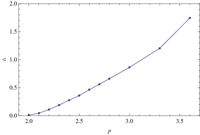
Finally, we show the relation between the width of the gap and . Evidently, the gap becomes wider as increases.
V Conclusions and discussion
In this paper, we have explored the fermionic response in the presence of a bulk dipole interaction term with strength in the dilatonic black brane with a Lifshitz like IR geometry and boundary. When , a sharp quasiparticle-like peak occurs near and , indicating a Fermi surface. As increases, the peak become wide and its strength degrades gradually, and the spectral weight is transferred between bands. Furthermore, when goes beyond a critical dipole interaction , the Fermi sea disappears and a gap emerges as the case in RN black hole [4]. By studying the another important quantity: the density of states , we clearly find that the onset of the gap is near and the width of the gap becomes bigger as increases.
So far, we have found a (Mott) gap from holographic fermions in the background of the dilatonic black brane with a Lifshitz like IR geometry when a dipole interaction term are added as that found in RN black hole. However, for more general dilatonic black brane, which also have vanishing ground entropy density, for example, a class of systems proposed in Refs.[21, 32, 33, 34], is the emergence of gap robust? The fermionic response without dipole interaction in this class backgrounds has been investigated in Refs.[24, 35]. Therefore, it is valuable to test the robustness of the emergence of the gap in the backgrounds of more general dilatonic black branes. In addition, it is also interesting to extend our investigations in this paper to the case of the non-relativistic fermionic fixed point. We will address them in the near future.
Acknowledgements.
We especially thank Professor Robert Leigh for his very valuable correspondence. J.P. Wu would also like to thank Hongbao Zhang and Wei-Jia Li for their collaboration in the related project. We also thank the referee for many valuable comments and correcting some English language typos. J.P. Wu is partly supported by NSFC(No.10975017) and the Fundamental Research Funds for the central Universities. H.B. Zeng is supported by the Fundamental Research Funds for the Central Universities (Grant No.1107020117) and the China Postdoctoral Science Foundation (Grant No. 20100481120).References
- [1] J. M. Maldacena, The large N limit of superconformal field theories and supergravity, Adv. Theor. Math. Phys. 2, 231 (1998) [Int. J. Theor. Phys. 38, 1113 (1999)], [hep-th/9711200].
- [2] S. S. Gubser, I. R. Klebanov, and A. M. Polyakov, Gauge theory correlators from non-critical string theory, Phys. Lett. B 428 (1998) 105¨C114, [hep-th/9802109].
- [3] E. Witten, Anti-de Sitter space and holography, Adv. Theor. Math. Phys. 2 (1998) 253¨C291, [hep-th/9802150].
- [4] H. Liu, J. McGreevy and D. Vegh, Non-Fermi Liquids from Holography, Phys. Rev. D 83, 065029 (2011), [arXiv:0903.2477].
- [5] Sung-Sik Lee, A Non-Fermi Liquid from a Charged Black Hole; A Critical Fermi Ball, Phys. Rev. D 79, 086006, (2009), [arXiv:0809.3402].
- [6] T. Faulkner, H. Liu, J. McGreevy and D. Vegh, Emergent Quantum Criticality, Fermi Surfaces, and , [arXiv:0907.2694].
- [7] T. Albash, C. V. Johnson, Landau Levels, Magnetic Fields and Holographic Fermi Liquids, J. Phys. A: Math. Theor. 43 (2010) 345404, [ arXiv:1001.3700].
- [8] P. Basu, J. Y. He, A. Mukherjee, H. H. Shieh, Holographic Non-Fermi Liquid in a Background Magnetic Field, Phys. Rev. D 82, 044036 (2010), [arXiv:0908.1436].
- [9] E. Gubankova, J. Brill, M. ubrovi, K. Schalm, P. Schijven, J. Zaanen, Holographic fermions in external magnetic fields, [arXiv:1011.4051].
- [10] M. ubrovi, J. Zaanen, K. Schalm, String theory, quantum phase transitions and the emergent Fermi-liquid, [arXiv:0904.1993].
- [11] D. Maity, S. Sarkar, B. Sathiapalan, R. Shankar and N. Sircar, Properties of CFTs dual to Charged BTZ black-hole, Nucl. Phys. B 839 (2010) 526-551, [arXiv:0909.4051].
- [12] J. P. Wu, Holographic fermions in charged Gauss-Bonnet black hole, JHEP 1107 106 (2011), [arXiv:1103.3982].
- [13] M. Alishahiha, M. Reza Mohammadi Mozaffar, A. Mollabashi, Fermions on Lifshitz Background, [arXiv:1201.1764].
- [14] L. Q. Fang, X. H. Ge, X. M. Kuang, Holographic fermions in charged Lifshitz theory, [arXiv:1201.3832].
- [15] N. Iqbal, H. Liu and M. Mezei, Lectures on holographic non-Fermi liquids and quantum phase transitions, [arXiv:1110.3814].
- [16] M. Edalati, R. G. Leigh, P. W. Phillips, Dynamically Generated Gap from Holography: Mottness from a Black Hole, Phys. Rev. Lett. 106, 091602 (2011), [ arXiv:1010.3238].
- [17] M. Edalati, R. G. Leigh, K. W. Lo, P. W. Phillips, Dynamical Gap and Cuprate-like Physics from Holography, Phys. Rev. D 83, 046012 (2011), [arXiv:1012.3751].
- [18] I. Bah, A. Faraggi, J. I. Jottar, R. G. Leigh, L. A. Pando Zayas, Fermions and D=11 Supergravity On Squashed Sasaki-Einstein Manifolds, JHEP 1102:068,2011, [arXiv:1008.1423].
- [19] I. Bah, A. Faraggi, J. I. Jottar, R. G. Leigh, Fermions and Type IIB Supergravity On Squashed Sasaki-Einstein Manifolds, JHEP 1101:100,2011, [arXiv:1009.1615].
- [20] D. Guarrera, J. McGreevy, Holographic Fermi surfaces and bulk dipole couplings, [arXiv:1102.3908].
- [21] S. S. Gubser, F. D. Rocha, Peculiar properties of a charged dilatonic black hole in , Phys. Rev. D 81, 046001 (2010), [arXiv:0911.2898].
- [22] K. Goldstein, S. Kachru, S. Prakash and S. P. Trivedi, Holography of Charged Dilaton Black Holes, JHEP 1008:078,2010, [arXiv:0911.3586].
- [23] C. P. Herzog, I. R. Klebanov, S. S. Pufu, T. Tesileanu, JHEP 1003, 093 (2010), [arXiv:0911.0400].
- [24] J. P. Wu, Some properties of the holographic fermions in an extremal charged dilatonic black hole, Phys. Rev. D 84 064008, (2011), [arXiv:1108.6134].
- [25] M. Cadoni, G. D’Appollonio, P. Pani, Phase transitions between Reissner-Nordstrom and dilatonic black holes in 4D AdS spacetime, JHEP 1003:100,2010, [arXiv:0912.3520].
- [26] M. Cadoni, P. Pani, Holography of charged dilatonic black branes at finite temperature, JHEP 1104:049,2011, [arXiv:1102.3820].
- [27] J. N. Laia, D. Tong, A Holographic Flat Band, [arXiv:1108.1381].
- [28] W. J. Li, H. Zhang, Holographic non-relativistic fermionic fixed point and bulk dipole coupling, JHEP, 1111, 018 (2011), [arXiv:1110.4559].
- [29] N. Iqbal and H. Liu, Fortsch. Phys. 57, 367 (2009), [arXiv:0903.2596].
- [30] M. Henningson and K. Sfetsos, Spinors and the AdS/CFT correspondence, Phys. Lett. B 431, 63 (1998), [arXiv:hep-th/9803251].
- [31] W. Mueck and K. S. Viswanathan, Conformal Field Theory Correlators from Classical Field Theory on Anti-de Sitter Space II. Vector and Spinor Fields, Phys. Rev. D 58, 106006 (1998), [arXiv:hep-th/9805145].
- [32] C. Charmousis, B. Gouteraux, B. S. Kim, E. Kiritsis and R. Meyer, Effective Holographic Theories for low-temperature condensed matter systems, JHEP 1011, 151 (2010) [arXiv:1005.4690].
- [33] R. Meyer, B. Gouteraux, B. S. Kim, Strange Metallic Behaviour and the Thermodynamics of Charged Dilatonic Black Holes, [arXiv:1102.4433].
- [34] B. Gouteraux, B. S. Kim, R. Meyer, Charged Dilatonic Black Holes and their Transport Properties, [arXiv:1102.4440].
- [35] N. Iizuka, N. Kundu, P. Narayan, S. P. Trivedi, Holographic Fermi and Non-Fermi Liquids with Transitions in Dilaton Gravity, [arXiv:1105.1162].