The nontrivial zeros of period polynomials of modular forms lie on the unit circleThanks: Research of the first two authors supported by the American Institute of Mathematics and the National Science Foundation, the research of the third author is supported by Swiss National Science Foundation

J. Brian Conrey, David W. Farmer, and Özlem Imamoglu Address: American Institute of Mathematicsconrey@aimath.orgfarmer@aimath.orgDepartment of MathematicsETH Zurichozlem@math.ethz.ch

Abstract.

We show that all but 5 of the zeros of the period polynomial associated to a Hecke cusp form are on the unit circle.

1. Introduction

Let ${\mathcal{M}}_{k}(\Gamma)$ be the space of holomorphic modular forms of weight $k$ for the full modular group $\Gamma=\operatorname{PSL}(2,\mathbb{Z})$ . It is well known that ${\mathcal{M}}_{k}(\Gamma)$ has dimension $\frac{k}{12}+O(1)$ and a modular form $f\in{\mathcal{M}}_{k}$ has $\frac{k}{12}+O(1)$ inequivalent zeros in a fundamental domain $\Gamma\backslash\mathcal{H}.$ The study of the natural question of the distribution of the zeros of modular forms dates back to the 1960’s and has seen some renewed interest thanks to the recent progress on the Quantum Unique Ergodicity (QUE) conjecture.

In the simplest case of Eisenstein series, it was conjectured by R.A. Rankin in 1968 and proved by F.K.C. Rankin and Swinnerton-Dyer [12] that all the zeros, in the standard fundamental domain, of the series

E_{k}(z)=\frac{1}{2}\sum_{(c,d)=1}(cz+d)^{-k}

lie on the geodesic arc $\{z\in\mathcal{H}\ :\ |z|=1,0\leq\Re{z}\leq 1/2\}$ and as $k\rightarrow\infty$ they become uniformly distributed on this unit arc. A similar result for the cuspidal Poincare series was proved by R.A. Rankin [13]. For generalizations of these results to other Fuchsian groups and to weakly holomorphic modular functions see [1], [3], [7], among many others.

In contrast to these cases, for the cuspidal Hecke eigenforms, it is a consequence of the recent proof of the holomorphic Quantum Unique Ergodicity(QUE) conjecture by Holowinsky and Soundararajan [8] that the zeros are uniformly distributed. More precisely, we have

Theorem.

(Holowinsky and Soundararajan [8]) Let $\{f_{k}\}$ be a sequence of cuspidal Hecke eigenforms. Then as $k\rightarrow\infty$ the zeros of $f_{k}$ become equidistributed with respect to the normalized hyperbolic measure $\frac{3}{\pi}\frac{dxdy}{y^{2}}$

For some recent work on the zeros of holomorphic Hecke cusp forms that lie on the geodesic segments of the standard fundamental domain see [5].

In this note we turn our attention from the zeros of modular forms to the zeros of their period polynomials.

It is well known that $\Gamma$ is generated by the elliptic transformations $S=\pm\left(\begin{smallmatrix}0&1\\ -1&0\end{smallmatrix}\right)$ and $U=\pm\left(\begin{smallmatrix}1&-1\\ 1&0\end{smallmatrix}\right)$ with the defining relations $S^{2}=U^{3}=\pm 1.$

Let $P_{k-2}$ be the space of all complex polynomials of degree at most $k-2$ . For $p(z)\in P_{k-2}$ , $A\in\operatorname{PSL}(2,\mathbb{C})$ acts on $p(z)$ in the usual way via

(p|A)(z):=(cz+d)^{k-2}p\left(\frac{az+b}{cz+d}\right)

Let $P^{-}_{k-2}$ be the space of odd polynomials of degree $k-2$ and

W^{-}=W^{-}_{k-2}=\{p\in P^{-}_{k-2};p|(1+S)=p|(1+U+U^{2})=0\}.

For $f(z)=\sum_{n=1}^{\infty}a(n)e^{2\pi inz}$ a Hecke eigenform of even integral weight $k=w+2$ and level 1, let $L_{f}(s)=\sum_{n=1}^{\infty}a(n)n^{-s}$ be its associated $L$ -function. The odd period polynomial for $f$ is defined by

r_{f}^{-}(X):=\sum_{n=1\atop n\mathrm{odd}}^{w-1}(-1)^{\frac{n-1}{2}}{w\choose n}n!(2\pi)^{-n-1}L_{f}(n+1)X^{w-n}.

(1.1)

The basic result of Eichler Shimura theory is

Theorem (Eichler-Shimura).

Let $\mathcal{S}_{k}(\Gamma)$ be the space of cusp form for $\Gamma$ . Then the map

	$\displaystyle r^{-}:\mathcal{S}_{k}(\Gamma)$	$\displaystyle\rightarrow W^{-}$
	$\displaystyle f$	$\displaystyle\rightarrow r_{f}^{-}(X)$

is an isomorphism.

In the light of the Theorem of Eichler and Shimura, studying the zeros of period polynomials is as natural as studying the zeros of modular forms. In this paper we prove

Theorem 1.1.

If $f$ is a Hecke eigenform, then the odd period polynomials $r_{f}^{-}(X)$ have simple zeros at $0,\pm 2$ ,and $\pm 1/2$ and double zeros at $\pm 1$ . The rest of its zeros are complex numbers on the unit circle.

Figure 1.1 illustrates Theorem 1.1 in the case of $f$ a cusp form of weight $w=34$ . Note that in this example the spacing between zeros is quite regular. From the proof of the Theorem 1.1 it will become clear that this is a general phenomenon. It is worth noting that for an arbitrary cusp form which is not a Hecke eigenform the zeros of $r_{f}^{-}(X)$ need not be on the unit circle. This can be thought as analogous to the fact that for a general modular form $f$ which is not a Hecke eigenform, the distribution of zeros of $f$ need not be uniformly distributed.

Refer to caption — Figure 1.1. A contour plot of $\log|r_{f}^{-}(z))$ for $f$ one of the cusp forms of weight $w=34$ , illustrating the zeros at $\pm 2$ , $\pm\frac{1}{2}$ , and $0$ , with the remaining zeros on the unit circle.

In the case of zeros of modular forms, the uniform distribution result is a remarkable consequence of the deep QUE conjecture, which is now a theorem due to Holowinsky and Soundararajan for holomorphic eigenforms. The fact that the uniform distribution of the zeros of modular forms follows from the QUE conjecture was first observed by S. Nonnenmacher and A. Voros [11], B. Shiffman and S. Zelditch [15] and Z. Rudnick [14].

In the case of the zeros of period polynomials, as we will show in the next section, Theorem 1.1 follows using simple function theory arguments together with the deep theorem of Deligne which is the Petersson-Ramanujan conjecture in the case of holomorphic cuspforms.

Finally it is worth noting that the proof of our Theorem 1.1 can be applied without much difficulty to show that the zeros of some special period polynomials are also on the unit circle. More precisely these are the polynomials associated to the cusp forms $R_{n}(z)$ , $0\leq n\leq w=k-2$ characterized by the property

r_{n}(f):=n!(2\pi)^{n-1}L(f,n+1)=(f,R_{n}),\,\,\,\forall f\in S_{k}(\Gamma).

Here $(f,R_{n})$ is the Petersson inner product of $f$ and $R_{n}$ . $R_{n}(z)$ has the following Poincare type series representation, due to H.Cohen [2]. For $0<n<w$ , ${\tilde{n}}=w-n$ and $c_{k,n}=i^{{\tilde{n}}+1}2^{-w}{w\choose n}\pi$ , we have

R_{n}(z)=c_{k,n}^{-1}\sum_{\left(\begin{smallmatrix}a&b\\ c&d\end{smallmatrix}\right)\in\Gamma}(az+b)^{-n-1}(cz+d)^{-{\tilde{n}}-1}

A special case of Theorem 1 in [9] gives that the odd period polynomial of $R_{n}$ for $n$ even and $0<n<w$ is given by the Bernoulli type polynomial

(-1)^{k/2+n/2}2^{-w}r^{-}_{R_{n}}(X)=\left[\frac{B^{0}_{\tilde{n}+1}(X)}{\tilde{n}+1}-\frac{B^{0}_{n+1}(X)}{n+1}\right]\mid(I-S)

(1.2)

where

B^{0}_{n+1}(X)=\sum_{\begin{subarray}{c}i=0\\ i\neq 1\end{subarray}}^{n+1}{n\choose i}B_{i}X^{n+1}.

The polynomials in (1.2) can also be closely approximated by $\sin(2\pi x)+x^{N}\sin(2\pi/x)$ which then can be used to show that their non-trivial zeros are on the unit circle. The period polynomials of the cusp forms $R_{n}$ can be seen as complementary to the Ramanujan polynomials which can be thought in terms of the period polynomials of the Eisenstein series. (see [9] and [4]) Recently, it was shown by R. Murty, C. Smyth, and R. Wang [10] that the zeros of the Ramanujan polynomials also lie on the unit circle. In this context see also [6].

2. Period polynomial of Hecke eigenforms

For $f(z)=\sum_{n=1}^{\infty}a(n)e^{2\pi inz}\in\mathcal{S}_{k}(\Gamma)$ , a Hecke eigenform, we let $L_{f}(s)=\sum_{n=1}^{\infty}a(n)n^{-s}$ be its associated $L$ -function and

r_{f}^{-}(X):=\sum_{n=1\atop n\mathrm{odd}}^{w-1}(-1)^{\frac{n-1}{2}}{w\choose n}n!(2\pi)^{-n-1}L_{f}(n+1)X^{w-n}.

(2.1)

the odd part of its period polynomial.

The L-function satisfies the functional equation

(2\pi)^{-s}\Gamma(s)L_{f}(s)=(-1)^{k/2}(2\pi)^{s-k}\Gamma(k-s)L_{f}(k-s).

It follows from the functional equation that $r_{f}^{-}(X)$ is self-reciprocal, i.e.

\displaystyle r_{f}^{-}(X)=X^{w}r_{f}^{-}(1/X)

(2.2)

and it follows from the modularity of $f$ (specifically that $f\big(\frac{z-1}{z}\big)=z^{k}f(z)$ ) that

r_{f}^{-}(X)+X^{w}r_{f}^{-}\big(1-\frac{1}{X}\big)+(X-1)^{w}r_{f}^{-}\big(\frac{-1}{X-1}\big)=0.

(2.3)

By Eichler Shimura theory the vector space of polynomials of degree less than or equal to $k-2$ spanned by the set of $r_{f}^{-}(X)$ as $f$ runs through Hecke eigenforms of weight $k$ is precisely the space of odd polynomials $P$ of degree $\leq k-3$ for which

P(x)+x^{k-2}P\big(\frac{-1}{x}\big)\equiv 0

(2.4)

and

P(x)+x^{k-2}P\big(1-\frac{1}{x}\big)+(x-1)^{k-2}P\big(\frac{-1}{x-1}\big)\equiv 0.

(2.5)

Lemma 2.1.

The polynomial $p$ in Theorem 1.1 has “trivial zeros” at $\pm 2$ , $\pm\frac{1}{2}$ , and $0$ .

Proof.

Since $P$ is odd, we have $P(0)=0$ and we only have to verify that $P(1)=P^{\prime}(1)=P(2)=P(1/2)=0$ . We substitute $x=1$ into (2.5), noting that

\displaystyle\lim_{x\to 1}(x-1)^{k-2}P\big(\frac{-1}{x-1}\big)=0

since $P$ has degree smaller than $k-2$ . Thus, $P(1)=0=P(-1)$ . Now we substitute $x=-1$ into (2.5) to obtain

P(2)+2^{k-2}P(1/2)=0

while from $x=2$ in (2.4) we have

P(2)-2^{k-2}P(1/2)=0.

Thus, $P(1/2)=P(2)=0$ . We differentiate (2.4) to obtain

P^{\prime}(x)+(k-2)x^{k-3}P\big(\frac{-1}{x}\big)+x^{k-4}P^{\prime}\big(\frac{-1}{x}\big)\equiv 0.

Substituting $x=1$ here gives

P^{\prime}(1)+P^{\prime}(-1)=0.

But $P$ is odd, so $P^{\prime}$ is even which means that $P^{\prime}(-1)=P^{\prime}(1)$ . Therefore, $P^{\prime}(1)=P^{\prime}(-1)=0$ and so we have verified that all of the trivial zeros are where we said they would be. ∎

To understand the rest of the zeros, we look at

	$\displaystyle p_{k}(X):=\frac{2\pi r_{f}^{-}(X)}{(-1)^{w/2}(2\pi)^{-w}(w-1)!}=\mathstrut$	$\displaystyle\sum_{n=1\atop n\mathrm{odd}}^{w-1}(-1)^{\frac{n-1}{2}}\frac{(2\pi X)^{n}}{n!}L_{f}(w-n+1)$		(2.6)
	$\displaystyle=\mathstrut$	$\displaystyle\sum_{m=0}^{w/2-1}\frac{(-1)^{m}(2\pi X)^{2m+1}}{(2m+1)!}L_{f}(w-2m).$		(2.7)

Since $L_{f}(w-2m)$ is close to 1 for small values of $m$ we see that the initial terms of the above are close to the initial terms of the series

\sin(2\pi X)=\sum_{m=0}^{\infty}\frac{(-1)^{m}(2\pi X)^{2m+1}}{(2m+1)!}.

The idea now is to study the zeros of

\sin(2\pi x)+x^{N}\sin(2\pi/x).

It follows from (2.2) that $p_{f}^{-}(X)$ may be written as

\displaystyle p_{f}^{-}(X)=q_{f}(X)+X^{w}q_{f}(1/X)

(2.8)

where

\displaystyle q_{f}(X)=\sum_{m=0}^{[(w-6)/4]}\frac{(-1)^{m}(2\pi X)^{2m+1}}{(2m+1)!}L_{f}(w-2m)+\frac{L_{f}\big(\frac{w+2}{2}\big)(2\pi X)^{\frac{w}{2}}}{2\big(\frac{w}{2}\big)!}.

(2.9)

Note that when $k\equiv 2\bmod 4$ the last term doesn’t appear, since in this case the functional equation implies that $L_{f}(k/2)=0$ . Note also that $q_{f}$ and $r_{f}^{-}$ have real coefficients, since $L_{f}(s)$ is real on the real axis.

To prove that the non trivial zeros of $r_{f}^{-}(X)$ are on the unit circle we need several lemmas. First we can replace $\sin 2\pi z$ above by an entire function $r(z)$ . The crucial idea is the following lemma.

Lemma 2.2.

Let $r(z)$ be an entire function and for $N\in\mathbb{N}$ let

F_{N}(z):=r(z)+z^{N}r(z^{-1}).

Let

R(\theta):=\Re{r(e^{i\theta})}\qquad\mathrm{and}\qquad I(\theta):=\Im{r(e^{i\theta})}.

For $j=0,\ldots 2M-1$ let $\mathcal{I}_{j}$ denote the interval $[\frac{\pi}{2M}+\frac{\pi}{M}j,\frac{\pi}{2M}+\frac{\pi}{M}(j+1)]\subset\mathbb{R}$ . Then

(1)

For $\theta_{j}=\frac{\pi}{2M}+\frac{\pi}{M}j$ , if $I(\theta_{j})=0$ , then $F_{2M}(e^{i\theta_{j}})=0$ .
(2)

If $I(\theta)\neq 0$ for $\theta\in\mathcal{I}_{j}$ , then $F_{2M}((e^{i\theta})=0$ for some $\theta\in\mathcal{I}_{j}$ .

Proof.

Let

f_{N}(z)=z^{-N/2}F_{N}(z)=z^{-M}r(z)+z^{M}r(z^{-1}),

where $2M=N$ . Note that $f_{N}$ and $F_{N}$ have the same zeros on $|z|=1$ . Since $f_{N}$ is real when $|z|=1$ , it suffices to look at the real valued function

\Re f_{N}(e^{i\theta})=2\cos(M\theta)R(\theta)+2\sin(M\theta)I(\theta)

(2.10)

Using $(\ref{re-part})$ , part $a)$ of the Lemma is clear.

To see part $b)$ note that If $I(\theta)\neq 0$ then $\Re f_{N}(e^{i\theta})=0$ will have a solution when

-\tan{M\theta}=\frac{R(\theta)}{I(\theta)}

(2.11)

If $I(\theta)\neq 0$ for $\theta\in\mathcal{I}_{j}$ then in the interval $\mathcal{I}_{j}$ the function $R(\theta)/I(\theta)$ is bounded and continuous and hence $(\ref{tan-eq})$ will have a solution. ∎

Lemma 2.3.

Let

S(z)=\sin(2\pi z)-\sin(2\pi/z).

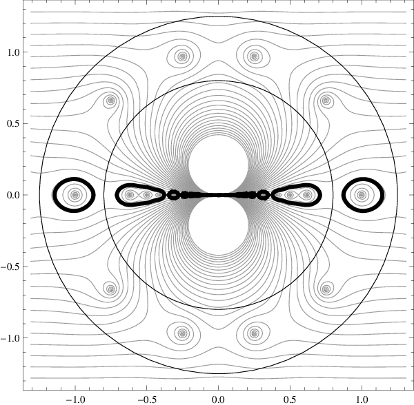
Then $S(z)$ has precisely 10 zeros in the annulus $A:=\{z:4/5\leq|z|\leq 5/4\}$ . Moreover, on the boundary of the annulus, $|S(z)|>1.$

This lemma can be verified with the aid of a graphing program such as Mathematica. One can plot the image of $S(z)$ on the boundary of $A$ and use the argument principle, or view a contour plot as shown in Figure 2.1.

Lemma 2.4.

Let $f$ be a Hecke eigenform of weight $k$ for the full modular group and let $L_{f}(s)=\sum a_{f}(n){n^{s}}$ be its associated L-function. Then for $\sigma\geq 3k/4$ , we have

\displaystyle|L_{f}(\sigma)-1|\leq 4\times 2^{-k/4}

(2.12)

and for $\sigma$ an integer with $\sigma\geq k/2$ , we have

\displaystyle L_{f}(\sigma)\leq 2k^{1/2}\log 2k+1.

(2.13)

Proof.

If $\sigma\geq 3k/4$ then we are in the region of absolute convergence. By Deligne’s Theorem we have

\displaystyle|L_{f}(\sigma)-1|\leq\sum_{n=2}^{\infty}\frac{d(n)}{n^{\sigma-(k-1)/2}}\leq\sum_{n=2}^{\infty}\frac{d(n)}{n^{k/4}}=\zeta(k/4)^{2}-1\leq 2(\zeta(k/4)-1).

We have

\displaystyle\zeta(k/4)-1=2^{-k/4}+\sum_{n=3}^{\infty}n^{-k/4}\leq 2^{-k/4}+\int_{2}^{\infty}u^{-k/4}~du\leq 2\times 2^{-k/4}

for $k\geq 12$ . This proves (2.12).

Next, if $\sigma\geq k/2+1$ we estimate $L_{f}(\sigma)$ trivially by $L_{f}(\sigma)\leq\zeta(3/2)^{2}<7$ . If $k/2\leq\sigma\leq k/2+1$ , then using standard methods, we have for $\sigma=k/2$ ,

\displaystyle\Gamma(k/2)L_{f}(k/2)=2\sum_{n=1}^{\infty}\frac{a_{f}(n)}{n^{k/2}}\int_{2\pi n}^{\infty}e^{-x}x^{k/2}\frac{dx}{x}.

Thus

\displaystyle|L_{f}(\sigma)|\leq 2\Gamma(k/2)^{-1}\sum_{n=1}^{\infty}\frac{d(n)}{n^{1/2}}\int_{2\pi n}^{\infty}e^{-x}x^{k/2}\frac{dx}{x}.

We split the sum over $n$ at $k$ . The terms with $n\leq k$ are

\displaystyle\leq\sum_{n\leq k}\frac{d(n)}{n^{1/2}}

as is seen by completing the integrals down to 0. Now

\displaystyle\sum_{n\leq k}\frac{d(n)}{n^{1/2}}=\sum_{mn\leq k}\frac{1}{(mn)^{1/2}}\leq\sum_{m\leq k}\frac{1}{m^{1/2}}\int_{0}^{k/m}u^{-1/2}~du=2k^{1/2}\sum_{m\leq k}\frac{1}{m}\leq 2k^{1/2}\log 2k

for $k\geq 5$ . The tail of the series is

	$\displaystyle=2\Gamma(k/2)^{-1}\sum_{n=k+1}^{\infty}\frac{d(n)}{\sqrt{n}}\int_{2\pi n}^{\infty}e^{-x}x^{k/2}\frac{dx}{x}$
	$\displaystyle\leq 2\Gamma(k/2)^{-1}\sum_{n=k+1}^{\infty}\frac{d(n)}{\sqrt{n}}e^{-\pi n}\int_{2\pi n}^{\infty}e^{-x/2}x^{k/2}\frac{dx}{x}.$

The integral is

=2^{k/2}\int_{\pi n}^{\infty}e^{-x}x^{k/2}\frac{dx}{x}\leq 2^{k/2}\Gamma(k/2).

Using $d(n)\leq 2\sqrt{n}$ we have that the tail is

\leq 4\times 2^{k/2}\sum_{n=k+1}^{\infty}e^{-\pi n}\leq 4\times 2^{k/2}e^{-\pi k}<1.

Note that $2k^{1/2}\log 2k+1>7$ for $k\geq 3$ . The proof is complete. ∎

Lemma 2.5.

Let $q_{f}$ be as in (2.9). Then, for $z\leq 5/4$ and $k\geq 80$ we have

|\sin 2\pi z-q_{f}(z)|\leq\frac{1}{100}.

Proof.

We have

\sin 2\pi z=\sum_{m=0}^{\infty}(-1)^{m}\frac{(2\pi z)^{2m+1}}{(2m+1)!}

and

q_{f}(z)=\sum_{m=0}^{[(w-6)/4]}\frac{(-1)^{m}(2\pi z)^{2m+1}}{(2m+1)!}L_{f}(w-2m)+\frac{L_{f}\big(\frac{w+2}{2}\big)(2\pi z)^{\frac{w}{2}}}{2\big(\frac{w}{2}\big)!}.

Thus,

$\displaystyle\|\sin 2\pi z-q_{f}(z)\|$	$\displaystyle\leq$	$\displaystyle\sum_{m\leq w/8}\frac{(5\pi/2)^{2m+1}}{(2m+1)!}\|L_{f}(w-2m)-1\|$
		$\displaystyle\qquad+\sum_{w/8<m<w/4}\frac{(5\pi/2)^{2m+1}}{(2m+1)!}(\|L_{f}(w-2m)\|+1)$
		$\displaystyle\qquad\qquad+\sum_{m>w/4}\frac{(5\pi/2)^{2m+1}}{(2m+1)!}$
	$\displaystyle=$	$\displaystyle\Sigma_{1}+\Sigma_{2}+\Sigma_{3},$

say. Now by Lemma 2.4 we have

\displaystyle\Sigma_{1}\leq 4\times 2^{-k/4}\sum_{m\leq w/8}\frac{(5\pi/2)^{2m+1}}{(2m+1)!}\leq 4\times 2^{-k/4}\times e^{5\pi/2}.

We can combine estimates for $\Sigma_{2}$ and $\Sigma_{3}$ . Again using Lemma 2.4 we have

\displaystyle\Sigma_{2}+\Sigma_{3}\leq(2\sqrt{k}\log 2k+2)\sum_{w/8<m}\frac{(5\pi/2)^{2m+1}}{(2m+1)!}.

We can bound the sum using

	$\displaystyle\sum_{m=r+1}^{\infty}\frac{x^{m}}{m!}$	$\displaystyle=$	$\displaystyle\frac{x^{r+1}}{(r+1)!}\left(1+\frac{x}{r+2}+\frac{x^{2}}{(r+2)(r+3)}+\dots\right)$
		$\displaystyle\leq$	$\displaystyle\frac{x^{r+1}}{(r+1)!}\frac{1}{(1-\frac{x}{r+1})}=\frac{x^{r+1}}{r!(r+1-x)}<\frac{(ex)^{r+1}}{r^{r}(r+1-x)},$

the last line uses $r!>(r/e)^{r}$ . Using this above we have

\displaystyle\Sigma_{2}+\Sigma_{3}\leq(2\sqrt{k}\log 2k+2)\frac{(5\pi e/2)^{k/2+1}}{(k/2)^{k/2}(k/2+1-5\pi/2)}.

For $k\geq 80$ we have $\Sigma_{1}+\Sigma_{2}+\Sigma_{3}<0.01$ . ∎

Lemma 2.6.

If $k\geq 80$ , then the function

Q_{f}(z):=q_{f}(z)-q_{f}(1/z)

has at most 10 zeros in the annulus $A$ .

This follows from Rouché’s theorem using Lemmas 2.3 and 2.5.

Corollary 2.7.

If $k\geq 80$ , then

\Im q_{f}(e^{i\theta})

has at most 10 zeros in $0\leq\theta<2\pi$ . Moreover, $\Im q_{f}(e^{i\theta})=0$ at $\theta=0$ and at $\theta=\pi$ .

Proof.

If $z$ is on the unit circle, then $\Im q_{f}(z)=-iQ_{f}(z)$ so any zero of $\Im q_{f}(z)$ has to be a zero of $Q_{f}(z)$ . But $Q_{f}(z)$ has at most 10 zeros on the annulus $A$ of which the unit circle is a subset. Since $r_{f}(\pm 1)=0$ , we see from (2.8) that $q_{f}(\pm 1)=0$ , so $\Im q_{f}(e^{i\theta})=0$ for $\theta=0$ and $\theta=\pi$ . ∎

We now combine these lemmas to prove

Theorem 2.8.

Let $f$ be a cusp form of weight $k\geq 80$ for $\operatorname{SL}(2,\mathbb{Z}),w=k-2$ and $p_{f}^{-}(z)=q_{f}(z)+z^{w}q_{f}(1/z)$ be its odd period polynomial of degree $w-1$ . Then $p_{f}^{-}(z)$ has all but 5 of its zeros on the unit circle. The 5 trivial zeros of $p_{f}(z)$ are at $z=0,2,-2,1/2,-1/2$ . It has double zeros at $z=1,-1.$

Proof.

First recall that we have shown that each period polynomial has simple zeros at $z=0,2,-2,1/2,-1/2$ and double zeros at $1,-1$ . To prove that the rest of the zeros are on the unit circle we let $r(z)=q_{f}(z)$ and $N=w=k-2$ in Lemma 2.2.

By the Corollary there are 10 zeros of $\Im(q_{f}(e^{i\theta}))$ in the interval $[0,2\pi)$ and hence by part $b)$ of Lemma 2.2 for each of the $N-10$ intervals among the N intervals $\mathcal{I}_{j}=[\frac{\pi}{2M}+\frac{\pi}{M}j,\frac{\pi}{2M}+\frac{\pi}{M}(j+1)]$ , $j=0,N-1$ for which $\Im(q_{f}(e^{i\theta}))\neq 0$ , $p_{f}(e^{i\theta})=0$ for some $\theta\in\mathcal{I}_{j}$ This gives at least $N-10$ zeros on the unit circle. Among the 10 discarded intervals in which $\Im(q_{f}(e^{i\theta})$ vanish, we have also excluded the intervals that contain $\theta=0$ and $\theta=\pi$ where $p_{f}(z)$ has double zeros. Hence we have at least $N-10+4=w-6$ zeros on the unit circle. Since the degree of $p_{f}(z)$ is $w-1$ together with the 5 zeros at $z=0,2,-2,1/2,-1/2$ , this covers all the zeros and finishes the proof of the theorem. ∎

Finally Theorem 1.1 follows from Theorem 2.8 together with the fact that for the weights $k\leq 80$ the statement can be verified numerically.

References

[1] T. Asai, M. Kaneko, and H. Ninomiya, Zeros of certain modular functions and an application, Comment. Math. Univ. St. Paul. 46 (1997), 93–101.
[2] H. Cohen, Sur certaines sommes de séries liées aux périodes de formes modulaires, in Séminaire de théorie des nombres, Grenoble, 1981.
[3] W. Duke and P. Jenkins, On the zeros and coefficients of certain weakly holomorphic modular forms, Pure Appl. Math. Q. 4 (2008), no. 4, 1327-1340.
[4] S. Fukuhara, Generalized Dedekind Symbols associated with the Eisenstein series, PAMS, Volume 127, Number 9, 2561-2568.
[5] A. Ghosh and P. Sarnak, Real zeros of holomorphic Hecke cusp forms, http://arxiv.org/pdf/1103.3262.
[6] S. Gun, M.R. Murty, P. Rath, Transcendental values of certain Eichler integrals, Bull. London Math. Soc., doi:10.1112/blms/bdr031.
[7] H. Hahn, On the zeros of Eisenstein series for genus zero Fuchsian groups, Proc. Amer. Math. Soc. 135 (2007), no. 8, 2391-2401.
[8] R. Holowinsky and K. Soundararajan, Mass equidistribution for Hecke eigenforms. Ann. of Math. (2) 172 (2010), no. 2, 1517–1528.
[9] W. Kohnen and D. Zagier, Modular forms with rational periods. Modular forms (Durham, 1983), 197–249, Ellis Horwood Ser. Math. Appl.: Statist. Oper. Res., Horwood, Chichester, 1984.
[10] R. Murty, C. Smyth, and R. Wang, Zeros of Ramanujan Polynomials, J. Ramanujan Math. Soc. 26, (2011) 107–125.
[11] S. Nonnenmacher and A. Voros, Chaotic eigenfunctions in phase space, J. Statist. Phys. 92 (1998), no. 3-4, 431–518.
[12] F.K.C. Rankin and Swinnerton-Dyer, On the zeros of Eisenstein series, Bull. London Math. Soc. 2 (1970), 169–170.
[13] R. A. Rankin The zeros of certain Poincaré series, Compositio Math. 46 (1982), no. 3, 255Ð272.
[14] Z. Rudnick, On the asymptotic distribution of zeros of modular forms, Int. Math. Res. Not., 34, (2005), 2059–2074.
[15] B. Shiffman and S. Zelditch, Distribution of zeros of random and quantum chaotic sections of positive line bundles, Comm. Math. Phys. 200 (1999), no. 3, 661–683.