Asymptotic expansion of the solution of the steady Stokes equation with variable viscosity in a two-dimensional tube structure

G.Cardone Affiliation: University of Sannio, Department of Engineering Affiliation: Piazza Roma, 21, 84100 Benevento, Italy Affiliation: email: giuseppe.cardone@unisannio.it R.Fares G.P.Panasenko Affiliation: Laboratory of Mathematics of the University of Saint Etienne (LaMUSE), EA 3989 Affiliation: 23, rue P.Michelon, 42023 St. Etienne, France Affiliation: email: roula.fares@univ-st-etienne.fr; grigory.panasenko@univ-st-etienne.fr

Abstract

The Stokes equation with the varying viscosity is considered in a thin tube structure, i.e. in a connected union of thin rectangles with heights of order $\varepsilon<<1$ and with bases of order $1$ with smoothened boundary. An asymptotic expansion of the solution is constructed: it contains some Poiseuille type flows in the channels (rectangles) with some boundary layers correctors in the neighborhoods of the bifurcations of the channels. The estimates for the difference of the exact solution and its asymptotic approximation are proved.

Keywords: Stokes equation, thin tube structures, variable viscosity, asymptotic expansion, boundary layer correctors.

AMS Subject Classification (2000): 35B27, 35Q30, 76M45, 65N55.

1 Introduction

The blood circulation, the transport of cells and substances in the human body as well as some liquid-cooling systems and oil-recovery/oil-transport processes in engineering, are modeled by the equations of fluid motion posed in thin domains. The present paper studies the Stokes equation with varying viscosity in a tube structure. In two-dimensional case a tube structure¹¹ 1 see Fig.5 (or pipe-wise structure) is some connected union of thin rectangles with heights of order $\varepsilon$ and with bases of order $1$ with a smoothened boundary $(\cite[cite]{[\@@bibref{}{CRAS}{}{}]},\cite[cite]{[\@@bibref{}{pana2005}{}{}]})$ ; here $\varepsilon$ is a small positive parameter. An asymptotic expansion for the case of a constant viscosity have been constructed in [1]. It is ”compiled” of some Poiseuille flows inside the rectangles glued by some boundary layer solutions, in the neighborhood of the junctions. Here we consider a more general case when the viscosity is not constant but depends on a longitudinal variable for each rectangle. This situation models a blood flow in a vessel structure where the viscosity depends on the concentration of some substances diluted in blood or some blood cells. Indeed, the asymptotic analysis of the convection-diffusion equation set in such domains $(\cite[cite]{[\@@bibref{}{CaPaSi}{}{}]},\cite[cite]{[\@@bibref{}{pana2005}{}{}]})$ shows that in the case of the Neumann (impermeability) condition at the lateral boundary and small Reynolds numbers, the concentration is asymptotically close to the one-dimensional description, that is the convection-diffusion equation set on the graph. The solution of the problem on the graph is the leading term of the asymptotic expansion, and it evidently on depends on the longitudinal variable. On the other hand, the viscosity often depends on the concentration of the diluted substances or distributed cells, and so, it depends on the longitudinal variable. Of course, the fluid motion equation is coupled with the diffusion-convection equation in this case. However, if the velocity is small (in our case, it is of order $\varepsilon^{2}$ ), then neglecting the convection, in comparison with the diffusion term or iterating with respect to the small term ²² 2 The simplest coupled diffusion-convection equation is $\begin{array}[c]{l}-\mathrm{div}(\nu(C_{\varepsilon}){\mathcal{D}}u_{\varepsilon})+\nabla p_{\varepsilon}=f(x)\\ \mathrm{div}u_{\varepsilon}=0,\\ -\Delta C_{\varepsilon}+u_{\varepsilon}.\nabla C_{\varepsilon}=0\end{array}$ where $C_{\varepsilon}$ is the concentration, $u_{\varepsilon}$ is the fluid velocity and $p_{\varepsilon}$ is the pressure.
If $u_{\varepsilon}$ is small with respect to $C_{\varepsilon}$ , we can write an expansion for $C_{\varepsilon}$ with respect to the small parameter that is the ratio of magnitudes of $|u_{\varepsilon}|$ and $|C_{\varepsilon}|$ . Then for the terms of this expansion, the third equation may be solved before the fluid motion equations. Another possible approach is the successive approximations (fixed point iterations) : $\begin{array}[c]{l}-\mathrm{div}(\nu(C^{(n)}_{\varepsilon}){\mathcal{D}}u^{(n)}_{\varepsilon})+\nabla p^{(n)}_{\varepsilon}=f(x)\\ \mathrm{div}u^{(n)}_{\varepsilon}=0,\\ -\Delta C^{(n)}_{\varepsilon}+u^{(n-1)}_{\varepsilon}.\nabla C^{(n)}_{\varepsilon}=0\end{array}$ where $n$ is the number of the iteration.
In both approaches, we get a problem with the variable viscosity., we get the steady state diffusion equation; in absence of the source term in the right hand side, it has a piecewise-linear asymptotic solution on the graph for the concentration. So, in this simplified situation, the diffusion equation can be solved before the fluid motion equation, and we obtain for the flow, the Stokes or Navier-Stokes equation with a variable viscosity depending (via concentration) on the longitudinal variable. These arguments provide the motivation for the Stokes equation with variable viscosity; to our knowledge, it has not been studied earlier from the asymptotic point of view.There are, of course, many other practical problems involving fluids with variable viscosity. For example, the presence of bacteria in suspension (see [6]) may change locally the viscosity.

In the first part, we consider the case of a flow in one rectangular channel with the periodicity condition at the end of the channel. An asymptotic expansion of solution is constructed and justified (a regular ansatz).

In the second part, we consider the case of a flow in one rectangular channel with the inflow/outflow boundary conditions at the ends. In this case as well we construct an asymptotic expansion of solution, that contains a regular ansatz and the boundary layer correctors.

In the third part, we construct an asymptotic expansion for solution of the Stokes equation set in a tube structure. Here as well we associate to each rectangle a regular ansatz and then we glue all the regular ansatzes with help of the boundary layer correctors exponential decaying from the junctions of rectangles. This procedure is similar to the procedure described in [10].

In the fourth part we consider some numerical experiments comparing the numerical and asymptotic solutions.

All constructed expansions are justified by calculation of residual terms and application of a priori estimates.

2 Flow in one channel

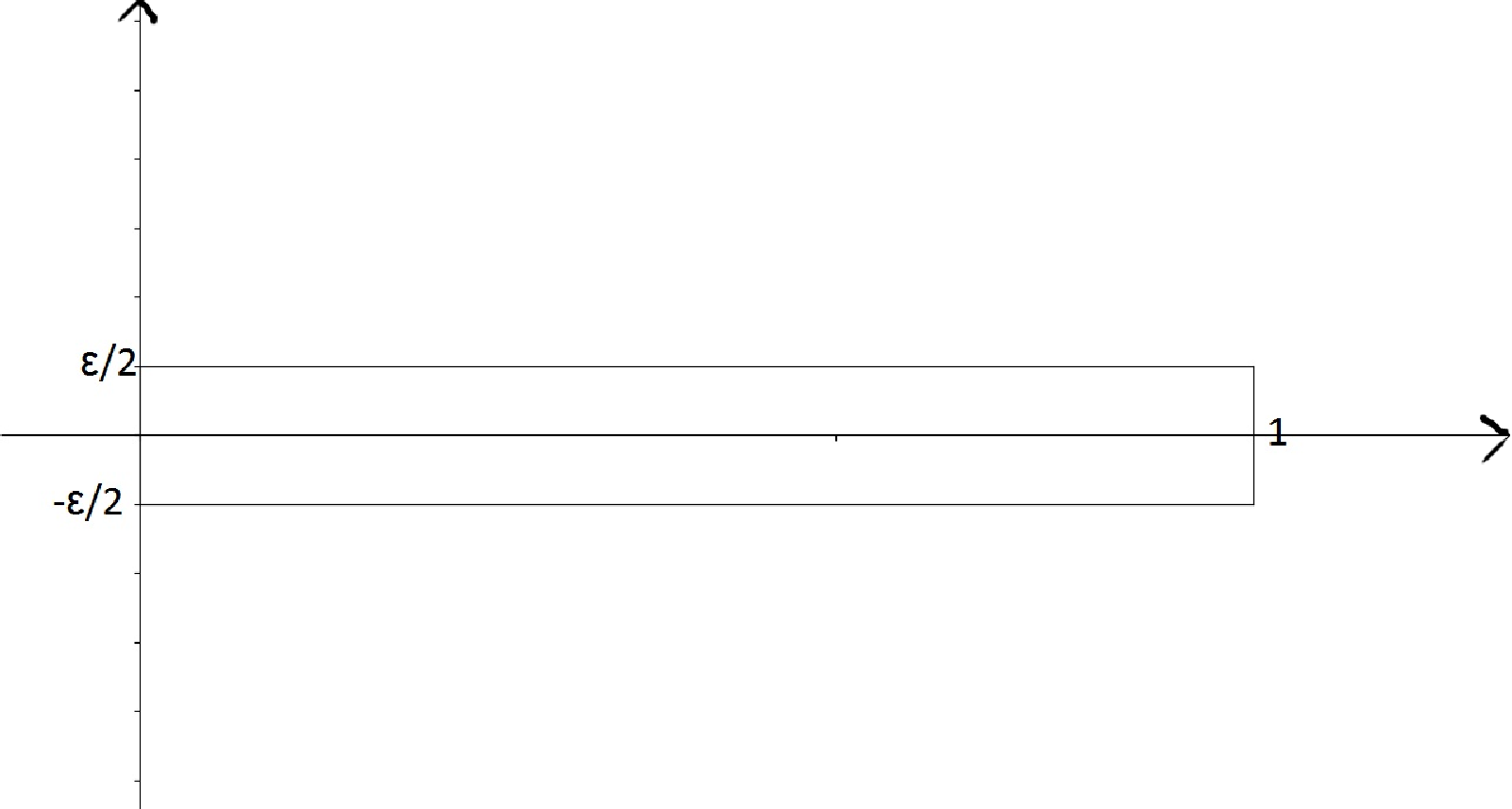
Consider a small parameter $\varepsilon$ , $\varepsilon=\frac{1}{q}$ , $q\in{\mathbb{N}}$ , and define then a thin domain

D_{\varepsilon}=\left\{(x_{1},x_{2})\in{\mathbb{R}}^{2}:0<x_{1}<1,\ -\frac{\varepsilon}{2}<x_{2}<\frac{\varepsilon}{2}\right\}.

Assume that incompressible, viscous fluid fills the domain $D_{\varepsilon}$ . Let $f$ be the exterior force applied to the fluid.

Refer to caption — Figure 1: Thin domain

Consider the following steady state Stokes problem:

\left\{\begin{array}[c]{ll}-\mathrm{div}(\nu(x_{1}){\mathcal{D}}u_{\varepsilon})+\nabla p_{\varepsilon}=f(x)&\text{in }D_{\varepsilon},\\ \mathrm{div}u_{\varepsilon}=0&\text{in }D_{\varepsilon},\\ u_{\varepsilon}(x_{1},\frac{\varepsilon}{2})=0&\text{for }x_{1}\in(0,1),\\ u_{\varepsilon}(x_{1},-\frac{\varepsilon}{2})=0&\text{for }x_{1}\in(0,1),\\ u_{\varepsilon}(0,x_{2})=\varepsilon^{2}\varphi_{0}(\frac{x_{2}}{\varepsilon})&\text{for }x_{2}\in(-\frac{\varepsilon}{2},\frac{\varepsilon}{2}),\\ u_{\varepsilon}(1,x_{2})=\varepsilon^{2}\varphi_{1}(\frac{x_{2}}{\varepsilon})&\text{for }x_{2}\in(-\frac{\varepsilon}{2},\frac{\varepsilon}{2}),\end{array}\right.

(1)

The unknowns of this system are the velocity $u_{\varepsilon}$ and the pressure $p_{\varepsilon}$ of the fluid.

The non homogeneous boundary conditions for the velocity are given by the functions $\varphi_{0},\varphi_{1}$ whose second component is equal to zero, and the first satisfies

\int_{-\frac{1}{2}}^{\frac{1}{2}}\varphi_{01}(\xi_{2})\mathrm{d}\xi_{2}=\int_{-\frac{1}{2}}^{\frac{1}{2}}\varphi_{11}(\xi_{2})\mathrm{d}\xi_{2},

(2)

where $\varphi_{i1}\in C_{0}^{2}([-\frac{1}{2},\frac{1}{2}])$ . Here $({\mathcal{D}}u_{\varepsilon})_{ij}=\frac{1}{2}\left(\frac{\partial u_{\varepsilon i}}{\partial x_{j}}+\frac{\partial u_{\varepsilon j}}{\partial x_{i}}\right)$ , $\nu$ satisfies the following conditions

\nu(x_{1})=\nu_{0}+\nu_{1}(x_{1})

(3)

where $\nu_{1}\in C_{0}^{2}([0,1])$ . Moreover there exist $\rho>0,$ $\kappa>0$ such that $\nu(x_{1})\geq\kappa$ for all $x_{1}\in(0,1)$ and $\nu_{1}(x_{1})=0$ for all $x_{1}\in(0,\rho)\cup(1-\rho,1)$ (and so, $\nu_{0}>0$ ).

2.1 Variational formulation of the problem

In order to obtain the variational formulation of problem (1), let us introduce the following space

H(D_{\varepsilon})=\left\{u\in(H_{0}^{1}(D_{\varepsilon}))^{2}:\mathrm{div}(u)=0\right\}

(4)

and assume that $f\in(L^{2}(D_{\varepsilon}))^{2}$ .

Applying the extension theorem (see [5]), one can find a function $\varphi^{\varepsilon}\in(H^{1}(D_{\varepsilon}))^{2}$ such that $\mathrm{div}\varphi^{\varepsilon}=0$ , $\varphi_{|_{x_{1}=0}}^{\varepsilon}=\varphi_{0}$ and $\varphi_{|_{x_{1}=1}}^{\varepsilon}=\varphi_{1}$ and $\varphi_{|_{x_{2}=\pm\frac{\varepsilon}{2}}}^{\varepsilon}=0$ . Changing the unknown function $u_{\varepsilon}$ by $v_{\varepsilon}=u_{\varepsilon}-\varepsilon^{2}\varphi^{\varepsilon},$ we give the variational formulation of problem (1):

\int_{D_{\varepsilon}}\nu(x_{1}){\mathcal{D}}v_{\varepsilon}:{\mathcal{D}}{\psi}=\int_{D_{\varepsilon}}f\cdot\psi-\varepsilon^{2}\int_{D_{\varepsilon}}\nu(x_{1}){\mathcal{D}}\varphi_{\varepsilon}:{\mathcal{D}}{\psi},\ \ \forall\psi\in H(D_{\varepsilon}).

(5)

Definition 2.1.

We say that $u_{\varepsilon}$ is a weak solution of problem (1) if $v_{\varepsilon}=u_{\varepsilon}-\varepsilon^{2}\varphi^{\varepsilon}\in H(D_{\varepsilon})$ and satisfies (5).

Proposition 2.1.

If $u_{\varepsilon}$ is a weak solution for problem (1), then there exists a distribution $p_{\varepsilon}\in{{\mathcal{D}}}^{{}^{\prime}}(D_{\varepsilon})$ such that $(u_{\varepsilon},p_{\varepsilon})$ satisfies (1)₁ this problem in sense of distributions.

Proof. If we take $v_{\varepsilon}=u_{\varepsilon}-\varepsilon^{2}\varphi^{\varepsilon}$ , then from $(5)$ we have that

\langle\mathrm{div}(\nu(x_{1}){\mathcal{D}}v_{\varepsilon}+\varepsilon^{2}\nu(x_{1}){\mathcal{D}}\varphi_{\varepsilon})+f,\psi\rangle=0,\forall\psi\in H(D_{\varepsilon})

From De Rham lemma, it follows that there exists a distribution $p_{\varepsilon}$ , unique up to an additive constant, such that

-\mathrm{div}(\nu(x_{1}){\mathcal{D}}v_{\varepsilon})+\varepsilon^{2}\mathrm{div}(\nu(x_{1}){\mathcal{D}}\varphi_{\varepsilon})-f=-\nabla p.

Theorem 2.1.

The variational problem (5) admits a unique solution $v_{\varepsilon}\in H(D_{\varepsilon})$ .

Proof. The Riesz’s theorem gives the existence and the uniqueness of solution because the norms $\|v_{\varepsilon}\|_{I}=\sqrt{\displaystyle{\int_{D_{\varepsilon}}\nu(x_{1}){\mathcal{D}}v_{\varepsilon}:{\mathcal{D}}v_{\varepsilon}}}$ and $\|v_{\varepsilon}\|_{(H^{1}_{0}(D_{\varepsilon}))^{2}}$ are equivalent.

As a consequence, we have:

Proposition 2.2.

Let $v_{\varepsilon}\in H(D_{\varepsilon})$ be the solution of the variational problem (5). Then the following inequality holds

\|v_{\varepsilon}\|_{(H(D_{\varepsilon}))^{2}}\leq{\mathcal{C}}(\kappa,C^{\varepsilon}_{PF})\left(\|f\|_{(L^{2}(D_{\varepsilon}))^{2}}+\|\varphi^{\varepsilon}\|_{\left(H^{1}(D_{\varepsilon})\right)^{2}}\right),

where $C^{\varepsilon}_{PF}$ stands for the Poincaré-Friedrichs inequality constant and $\kappa$ is the lower bound of the viscosity (3).

Mention that $C^{\varepsilon}_{PF}$ can be estimated by $\varepsilon\tilde{{\mathcal{C}}}$ , where $\tilde{{\mathcal{C}}}$ is independent of $\varepsilon$ (see [10]).

Consider the case when $\varphi^{\varepsilon}=0.$ Then we have:

Proposition 2.3.

The following inequality holds

\|\nabla p_{\varepsilon}\|_{H^{-1}(D_{\varepsilon})}\leq C\|f\|_{\left(L^{2}(D_{\varepsilon})\right)^{2}},

where $C$ is a constant independent of $\varepsilon.$

Proof. From De Rham lemma, it follows that there exists a distribution $p_{\varepsilon}$ , unique up to an additive constant, such that

\nabla p_{\varepsilon}=\mathrm{div}(\nu(x_{1}){\mathcal{D}}u_{\varepsilon})+f.

It means that

\int_{D_{\varepsilon}}p_{\varepsilon}\mathrm{div}\psi=\int_{D_{\varepsilon}}\nu(x_{1}){\mathcal{D}}u_{\varepsilon}:{\mathcal{D}}{\psi}-\int_{D_{\varepsilon}}f\cdot\psi,\quad\forall\psi\in H(D_{\varepsilon}))^{2},

and so,

\sup_{\psi\in(H^{1}_{0}(D_{\varepsilon}))^{2}}\frac{|\int_{D_{\varepsilon}}p_{\varepsilon}div\psi|}{\|\nabla\psi\|_{(L^{2}(D_{\varepsilon}))^{4}}}=\sup_{\psi\in(H^{1}_{0}(D_{\varepsilon}))^{2}}\frac{|\int_{D_{\varepsilon}}\nu(x_{1}){\mathcal{D}}u_{\varepsilon}:{\mathcal{D}}{\psi}-\int_{D_{\varepsilon}}f\cdot\psi|}{\|\nabla\psi\|_{(L^{2}(D_{\varepsilon}))^{4}}}\leq

\leq({\mathcal{C}}(\kappa,C^{\varepsilon}_{PF})+C^{\varepsilon}_{PF})\|f\|_{(L^{2}(D_{\varepsilon}))^{2}},

where ${\mathcal{C}}(\kappa,C^{\varepsilon}_{PF})$ is the constant of the a priori estimate for $u_{\varepsilon}$ (see above) and $C^{\varepsilon}_{PF}$ is the Poincaré-Friedrichs constant (it is of order $\varepsilon$ ). This inequality gives the estimate of $\nabla p_{\varepsilon}$ in the $H^{-1}-$ norm.

An asymptotic analysis of problem (1) shows that an asymptotic solution is given by a Poiseuille type flow, with two boundary layer correctors localized in some neighborhoods of the ends of the channel. Didactically, it would be better to separate the construction of the Poiseuille type flow for varying viscosity and the construction of the boundary layer correctors. That’s why we simplify problem (1), and replace $\eqref{1.1}_{5}$ , $\eqref{1.1}_{6}$ by the periodicity condition with respect to $x_{1}$ .

Introduce the Sobolev space

H_{per}(D_{\varepsilon})=\left\{u\in{\left(H_{per,1,0}^{1}(D_{\varepsilon})\right)}^{2}:\operatorname{div}u=0\right\}.

Here $H_{per,1,0}^{1}(D_{\varepsilon})$ is the completion (with respect to the $H^{1}(D_{\varepsilon})$ -norm) of the space of the $C^{\infty}({\mathbb{R}}\times[-\frac{\varepsilon}{2},\frac{\varepsilon}{2}])$ -functions vanishing at the boundary $x_{2}=\pm\frac{\varepsilon}{2}$ and 1-periodic in $x_{1}$ . As in the beginning of the section, $f\in(L^{2}(D_{\varepsilon}))^{2}$ .

Definition 2.2.

We say that $u_{\varepsilon}\in H_{per}(D_{\varepsilon})$ is a weak solution of the periodic problem

\left\{\begin{array}[c]{ll}-\mathrm{\operatorname{div}}(\nu(x_{1}){\mathcal{D}}u_{\varepsilon})+\nabla p_{\varepsilon}=f(x),&\text{in }D_{\varepsilon},\\ \mathrm{\operatorname{div}}u_{\varepsilon}=0,&\text{in }D_{\varepsilon},\\ u_{\varepsilon}(x_{1},\frac{\varepsilon}{2})=0,&\text{for }x_{1}\in(0,1),\\ u_{\varepsilon}(x_{1},-\frac{\varepsilon}{2})=0,&\text{for }x_{1}\in(0,1),\\ u_{\varepsilon}\text{ is }1-\text{periodic in }x_{1},&\end{array}\right.

(6)

if and only if it satisfies the integral identity

\int_{D_{\varepsilon}}\nu(x_{1}){\mathcal{D}}u_{\varepsilon}:{\mathcal{D}}{\psi}=\int_{D_{\varepsilon}}f\cdot\psi,\text{ \ }\forall\psi\in H_{per}(D_{\varepsilon}).

(7)

As in theorem 2.1, we apply the Riesz theorem and prove the existence and the uniqueness of $u_{\varepsilon}\in H_{per}(D_{\varepsilon})$ , solution of problem (6). The a priori estimate is given by

\|u_{\varepsilon}\|_{(H^{1}(D_{\varepsilon}))^{2}}\leq{\mathcal{C}}(\kappa,C^{\varepsilon}_{PF})\|f\|_{(L^{2}(D_{\varepsilon}))^{2}}

where ${\mathcal{C}}(\kappa,C^{\varepsilon}_{PF})=O\left(\varepsilon\right)$ and $\kappa$ is the lower bound of the viscosity (3).

Proposition 2.4.

If $u_{\varepsilon}$ is a weak solution for problem (6) then there exists a distribution $p_{\varepsilon}\in{{\mathcal{D}}}^{{}^{\prime}}(D_{\varepsilon})$ such that $(u_{\varepsilon},p_{\varepsilon})$ satisfies (6) ₁ in sense of distributions, and

\|\nabla p_{\varepsilon}\|_{H^{-1}(D_{\varepsilon})}\leq C\|f\|_{\left(L^{2}(D_{\varepsilon})\right)^{2}},

where $C$ is a constant independent of $\varepsilon.$

Proof. By (7)

\int_{D_{\varepsilon}}\nu(x_{1}){\mathcal{D}}u_{\varepsilon}:{\mathcal{D}}{\psi}=\int_{D_{\varepsilon}}f\cdot\psi,\qquad\forall\psi\in H_{per}(D_{\varepsilon}).

From De Rham lemma, it follows that there exists a distribution $p_{\varepsilon}$ , unique up to an additive constant, such that

\nabla p_{\varepsilon}=\mathrm{div}(\nu(x_{1}){\mathcal{D}}u_{\varepsilon})+f.

It means that

\int_{D_{\varepsilon}}p_{\varepsilon}\mathrm{div}\psi=\int_{D_{\varepsilon}}\nu(x_{1}){\mathcal{D}}u_{\varepsilon}:{\mathcal{D}}{\psi}-\int_{D_{\varepsilon}}f\cdot\psi\qquad\forall\psi\in(H^{1}_{per,1,0}(D_{\varepsilon}))^{2},

and so,

\sup_{\psi\in(H^{1}_{per,1,0}(D_{\varepsilon}))^{2}}\frac{|\int_{D_{\varepsilon}}p_{\varepsilon}\mathrm{div}\psi|}{\|\nabla\psi\|_{(L^{2}(D_{\varepsilon}))^{4}}}=\sup_{\psi\in(H^{1}_{per,1,0}(D_{\varepsilon}))^{2}}\frac{|\int_{D_{\varepsilon}}\nu(x_{1}){\mathcal{D}}u_{\varepsilon}:{\mathcal{D}}{\psi}-\int_{D_{\varepsilon}}f.\psi|}{\|\nabla\psi\|_{(L^{2}(D_{\varepsilon}))^{4}}}\leq

\leq({\mathcal{C}}(\kappa,C^{\varepsilon}_{PF})+C^{\varepsilon}_{PF})\|f\|_{(L^{2}(D_{\varepsilon}))^{2}},

2.2 Asymptotic analysis of the problem

Let us first construct the asymptotic expansion for the solution of the periodic problem (6); then we will study the non periodic one.

Define the infinite layer

\Omega_{\varepsilon}=\left\{(x_{1},x_{2})\in{\mathbb{R}}^{2}:x_{1}\in{\mathbb{R}},-\frac{\varepsilon}{2}<x_{2}<\frac{\varepsilon}{2}\right\}.

Assume that $f=f_{1}e_{1}$ , $f_{1}\in C^{\infty}({\mathbb{R}})$ , $f_{1}$ is 1-periodic in $x_{1}$ .

Denote ${\langle\psi\rangle}_{1}=\int_{0}^{1}\psi(x_{1},x_{2})\mathrm{d}x_{1}$ , $\langle\psi{\rangle}_{2}=\int_{-\frac{1}{2}}^{\frac{1}{2}}\psi(x_{1},x_{2})\mathrm{d}x_{2}$ . An asymptotic solution is written as:

\left\{\begin{array}[c]{lcl}u_{1}^{k}(x_{1},x_{2})&=&\displaystyle{\sum_{j=0}^{k}}\varepsilon^{j+2}u_{1,j}\left(x_{1},\frac{x_{2}}{\varepsilon}\right),\\ u_{2}^{k}(x_{1},x_{2})&=&\displaystyle{\sum_{j=0}^{k}}\varepsilon^{j+3}u_{2,j}\left(x_{1},\frac{x_{2}}{\varepsilon}\right),\\ p^{k}(x_{1},x_{2})&=&\displaystyle{\sum_{j=0}^{k}}\varepsilon^{j+1}p_{j}\left(x_{1},\frac{x_{2}}{\varepsilon}\right)+\displaystyle{\sum_{j=0}^{k}}\varepsilon^{j}q_{j}(x_{1}),\end{array}\right.

(8)

with $u_{1,j},u_{2,j},p_{j}$ and $q_{j}$ 1-periodic functions in $x_{1}$ , such that $\langle p_{j}\rangle_{2}=0$ .

Substituting (8), in (6), equating the coefficients of the same powers of $\varepsilon$ and denoting $\xi_{2}=\frac{x_{2}}{\varepsilon}$ we obtain:

\left\{\begin{array}[c]{l}-\frac{\partial}{\partial x_{1}}\left(\nu(x_{1})\frac{\partial u_{1,j-2}}{\partial x_{1}}\right)-\frac{\nu(x_{1})}{2}\frac{\partial^{2}u_{1,j}}{\partial\xi_{2}^{2}}-\frac{\nu(x_{1})}{2}\frac{\partial^{2}u_{2,j-2}}{\partial\xi_{2}\partial x_{1}}+\frac{\partial p_{j-1}}{\partial x_{1}}+\frac{\partial q_{j}}{\partial x_{1}}=f_{1}\delta_{j0},\\ \\ \frac{1}{2}\frac{\partial}{\partial x_{1}}\left[\nu(x_{1})\left(\frac{\partial u_{1,j-1}}{\partial\xi_{2}}+\frac{\partial u_{2,j-3}}{\partial x_{1}}\right)\right]+\nu(x_{1})\frac{\partial^{2}u_{2,j-1}}{\partial\xi_{2}^{2}}-\frac{\partial p_{j}}{\partial\xi_{2}}=0,\\ \\ \frac{\partial u_{1,j}}{\partial x_{1}}+\frac{\partial u_{2,j}}{\partial\xi_{2}}=0,\\ \\ u_{1,j}\left(x_{1},\pm\frac{1}{2}\right)=0,\\ \\ u_{2,j}\left(x_{1},\pm\frac{1}{2}\right)=0.\end{array}\right.

(9)

Denote:

N_{1}(\xi_{2})=\frac{1}{2}\left(\xi_{2}^{2}-\frac{1}{4}\right),

(it satisfies $N_{1}^{{}^{\prime\prime}}=1$ , $N_{1}(\pm\frac{1}{2})=0$ ) and

N_{2}(\xi_{2})=\int_{-\frac{1}{2}}^{\xi_{2}}N_{1}(\tau)\mathrm{d}\tau,

(here $N_{2}(\frac{1}{2})={{\displaystyle\int_{-\frac{1}{2}}^{\frac{1}{2}}}N_{1}(\tau)\mathrm{d}\tau}=-\frac{1}{12}$ ). Denote:

\left\{\begin{array}[c]{l}D^{-1}:F\longrightarrow\displaystyle{\int_{-\frac{1}{2}}^{\xi_{2}}F(x_{1},\tau)\mathrm{d}\tau,}\\ \tilde{D}^{-1}:F\longrightarrow\displaystyle{\int_{-\frac{1}{2}}^{\xi_{2}}F(x_{1},\tau)\mathrm{d}\tau-\int_{-\frac{1}{2}}^{\frac{1}{2}}\int_{-\frac{1}{2}}^{\theta}F(x_{1},\tau)\mathrm{d}\tau\mathrm{d}\theta,}\\ D^{-2}:F\longrightarrow\displaystyle{\int_{-\frac{1}{2}}^{\xi_{2}}\int_{-\frac{1}{2}}^{\theta}F(x_{1},\tau)\mathrm{d}\tau\mathrm{d}\theta-\left(\xi_{2}+\frac{1}{2}\right)\int_{-\frac{1}{2}}^{\frac{1}{2}}\int_{-\frac{1}{2}}^{\theta}F(x_{1},\tau)\mathrm{d}\tau\mathrm{d}\theta.}\end{array}\right.

Theorem 2.2.

The unknowns of (9) $u_{1,j},u_{2,j},p_{j},q_{j}$ are given by the following relations:

\left\{\begin{array}[c]{lcl}u_{1,j}&=&-D^{-2}\left\{\frac{\partial^{2}u_{2,j-2}}{\partial\xi_{2}\partial x_{1}}+\frac{2}{\nu(x_{1})}\left(\frac{\partial}{\partial x_{1}}\left(\nu(x_{1})\frac{\partial u_{1,j-2}}{\partial x_{1}}\right)-\frac{\partial p_{j-1}}{\partial x_{1}}\right)\right\}\\ &&+\frac{2}{\nu(x_{1})}N_{1}(\xi_{2})\left(\frac{\partial q_{j}}{\partial x_{1}}-f_{1}\delta_{j0}\right),\\ &&\\ u_{2,j}&=&D^{-1}D^{-2}\left\{\frac{\partial^{3}u_{2,j-2}}{\partial\xi_{2}\partial x_{1}^{2}}+\frac{\partial}{\partial x_{1}}\left(\frac{2}{\nu(x_{1})}\left(\frac{\partial}{\partial x_{1}}\left(\nu(x_{1})\frac{\partial u_{1,j-2}}{\partial x_{1}}\right)-\frac{\partial p_{j-1}}{\partial x_{1}}\right)\right)\right\}\\ &&-\frac{\partial}{\partial x_{1}}\left(\frac{2}{\nu(x_{1})}\left(\frac{\partial q_{j}}{\partial x_{1}}-f_{1}\delta_{j0}\right)\right)N_{2}(\xi_{2}),\\ &&\\ p_{j}&=&\tilde{D}^{-1}\left\{\frac{1}{2}\frac{\partial}{\partial x_{1}}\left[\nu(x_{1})\left(\frac{\partial u_{1,j-1}}{\partial\xi_{2}}+\frac{\partial u_{2,j-3}}{\partial x_{1}}\right)\right]+\nu(x_{1})\frac{\partial^{2}u_{2,j-1}}{\partial\xi_{2}^{2}}\right\}.\end{array}\right.

(10)

Proof. Integrating twice $\eqref{A.3}_{1}$ and using boundary conditions $\eqref{A.3}_{4}$ , we get $\eqref{A.4}_{1}$ . This relation gives an expression of the unknown $u_{1,j}$ via $q_{j}$ . All other functions contained by this relation are either known from previous computations or equal to zero. We integrate next the incompressibility condition $\eqref{A.3}_{3}$ with respect to $\xi_{2}$ with the boundary condition $\eqref{A.3}_{5}$ and get $u_{2,j}$ . Finally, integrating $\eqref{A.3}_{2}$ we get $p_{j}$ . The unknown function $q_{j}$ is determined from the boundary condition $u_{2,j}\left(x_{1},\frac{1}{2}\right)=0$ . Actually, the boundary conditions $\eqref{A.3}_{4}$ and $u_{2,j}\left(x_{1},-\frac{1}{2}\right)=0$ are satisfied by the definition of $D^{-2}$ and $D^{-1}$ , while $u_{2,j}\left(x_{1},\frac{1}{2}\right)=0$ gives:

	$\displaystyle-\frac{\partial}{\partial x_{1}}$	$\displaystyle\left(\frac{1}{6\nu(x_{1})}\left(\frac{\partial q_{j}}{\partial x_{1}}-f_{1}\delta_{j0}\right)\right)=$		(11)
		$\displaystyle={D^{-1}D^{-2}\left\{\frac{\partial^{3}u_{2,j-2}}{\partial\xi_{2}\partial x_{1}^{2}}+\frac{\partial}{\partial x_{1}}\left\{\frac{2}{\nu(x_{1})}\left(\frac{\partial}{\partial x_{1}}\left(\nu(x_{1})\frac{\partial u_{1,j-2}}{\partial x_{1}}\right)-\frac{\partial p_{j-1}}{\partial x_{1}}\right)\right\}\right\}}_{\left\|{}_{\xi_{2}=\frac{1}{2}}\right..}$

In particular, for $j=0$ , we have the Darcy equation for the leading term of the pressure $q_{0}$ :

\frac{\partial}{\partial x_{1}}\left(\frac{1}{6\nu(x_{1})}\left(\frac{\partial q_{0}}{\partial x_{1}}-f_{1}\right)\right)=0,

(12)

and so $q_{0}$ is the 1-periodic function given by the formula

q_{0}(x_{1})=\displaystyle{\int_{0}^{x_{1}}\left(f_{1}(\tau)-\frac{\langle f_{1}\rangle_{1}}{\langle\nu\rangle_{1}}\nu(\tau)\right)\mathrm{d}\tau-\left\langle\int_{0}^{x_{1}}\left(f_{1}(\tau)-\frac{\langle f_{1}\rangle_{1}}{\langle\nu\rangle_{1}}\nu(\tau)\right)\mathrm{d}\tau\right\rangle_{1}}.

Then $u_{1,0}(x_{1},\xi_{2})=\frac{2}{\nu(x_{1})}\left(\frac{\partial q_{0}}{\partial x_{1}}-f_{1}\right)N_{1}(\xi_{2})$ , $u_{2,0}(x_{1},\xi_{2})=0$ and $p_{0}(x_{1},\xi_{2})=0$ .
For $j=1$ $q_{1}$ is the 1-periodic solution of equation

\frac{\partial}{\partial x_{1}}\left(\frac{1}{6\nu(x_{1})}\frac{\partial q_{1}}{\partial x_{1}}\right)=0.

It follows: $q_{1}=0$ , $u_{1,1}(x_{1},\xi_{2})=0\mbox{ and }u_{2,1}(x_{1},\xi_{2})=0$ . For $j=1$ , $\eqref{A.4}_{3}$ yields:

p_{1}(x_{1},\xi_{2})=\frac{\partial}{\partial x_{1}}\left(\frac{\partial q_{0}}{\partial x_{1}}-f_{1}\right)\left(N_{1}(\xi_{2})-\langle N_{1}\rangle_{2}\right).

For $j=2$ , (11) becomes

\frac{\partial}{\partial x_{1}}\left(\frac{1}{6\nu(x_{1})}\frac{\partial q_{2}}{\partial x_{1}}\right)=\frac{\partial}{\partial x_{1}}\left(\frac{2}{\nu(x_{1})}\frac{\partial}{\partial x_{1}}\left(\frac{\partial q_{0}}{\partial x_{1}}-f_{1}\right)\right)D^{-1}D^{-2}\left(N_{1}(\xi_{2})-\langle N_{1}\rangle_{2}\right)_{\left|{}_{\xi_{2}=\frac{1}{2}}\right.},

(13)

where $D^{-1}D^{-2}\left(N_{1}(\xi_{2})-\langle N_{1}\rangle_{2}\right)_{\left|{}_{\xi_{2}=\frac{1}{2}}\right.}={\mathcal{R}}\neq 0$ , $q_{2}$ is 1-periodic solution of given by:

q_{2}(x_{1})=-12{\mathcal{R}}{\langle f_{1}\rangle_{1}}\left(\frac{\nu(x_{1})}{\langle\nu\rangle_{1}}-1\right).

It follows:

\left\{\begin{array}[c]{l}u_{1,2}(x_{1},\xi_{2})=\frac{2}{\nu(x_{1})}\frac{\partial^{2}}{\partial x_{1}^{2}}(\frac{\partial q_{0}}{\partial x_{1}}-f_{1})D^{-2}\left(N_{1}(\frac{x_{2}}{\varepsilon})-\langle N_{1}\rangle_{2}\right)+\frac{2}{\nu(x_{1})}N_{1}(\frac{x_{2}}{\varepsilon})\frac{\partial q_{2}}{\partial x_{1}},\\ \\ u_{2,2}(x_{1},\xi_{2})=-\frac{\partial}{\partial x_{1}}\left[\frac{2}{\nu(x_{1})}\frac{\partial^{2}}{\partial x_{1}^{2}}\left(\frac{\partial q_{0}}{\partial x_{1}}-f_{1}\right)\right]D^{-1}D^{-2}\left(N_{1}(\frac{x_{2}}{\varepsilon})-\langle N_{1}\rangle_{2}\right)-\frac{\partial}{\partial x_{1}}\left(\frac{2}{\nu(x_{1})}N_{2}(\frac{x_{2}}{\varepsilon})\frac{\partial q_{2}}{\partial x_{1}}\right),\end{array}\right.

and we get the following theorem.

Theorem 2.3.

The asymptotic solution of problem (6) is given by:

\left\{\begin{array}[c]{lcl}u_{1}^{k}(x_{1},x_{2})&=&\varepsilon^{2}\frac{2}{\nu(x_{1})}\left(\frac{\partial q_{0}}{\partial x_{1}}-f_{1}\right)N_{1}(\frac{x_{2}}{\varepsilon})\\ &&+\varepsilon^{4}\left(\frac{2}{\nu(x_{1})}\frac{\partial^{2}}{\partial x_{1}^{2}}(\frac{\partial q_{0}}{\partial x_{1}}-f_{1})D^{-2}\left(N_{1}(\frac{x_{2}}{\varepsilon})-\langle N_{1}\rangle_{2}\right)+\frac{2}{\nu(x_{1})}N_{1}(\frac{x_{2}}{\varepsilon})\frac{\partial q_{2}}{\partial x_{1}}\right)+O(\varepsilon^{5}),\\ &&\\ u_{2}^{k}(x_{1},x_{2})&=&-\varepsilon^{5}\left(\frac{\partial}{\partial x_{1}}\left[\frac{2}{\nu(x_{1})}\frac{\partial^{2}}{\partial x_{1}^{2}}\left(\frac{\partial q_{0}}{\partial x_{1}}-f_{1}\right)\right]D^{-1}D^{-2}\left(N_{1}(\frac{x_{2}}{\varepsilon})-\langle N_{1}\rangle_{2}\right)\right.\\ &&\left.+\frac{\partial}{\partial x_{1}}\left(\frac{2}{\nu(x_{1})}N_{2}(\frac{x_{2}}{\varepsilon})\frac{\partial q_{2}}{\partial x_{1}}\right)\right)+O(\varepsilon^{6}),\\ &&\\ p^{k}(x_{1},x_{2})&=&q_{0}+\varepsilon^{2}\left(q_{2}(x_{1})+\frac{\partial}{\partial x_{1}}\left(\frac{\partial q_{0}}{\partial x_{1}}-f_{1}\right)\left(N_{1}(\frac{x_{2}}{\varepsilon})-\langle N_{1}\rangle_{2}\right)\right)+O(\varepsilon^{3}),\end{array}\right.

(14)

where $q_{0}$ and $q_{2}$ are periodic solutions of obtained as the unique solution of (11) (13) respectively.

Remark 2.1.

Solution given by (14) can be written as follows:

\left\{\begin{array}[c]{lcl}u_{1}^{k}(x_{1},x_{2})&=&-\varepsilon^{2}\frac{2\langle f_{1}\rangle_{1}}{\langle\nu(x_{1})\rangle_{1}}N_{1}(\xi_{2})-\varepsilon^{4}\left(\frac{2}{\nu(x_{1})}\frac{\langle f_{1}\rangle_{1}}{\langle\nu\rangle_{1}}\nu^{{}^{\prime\prime}}(x_{1})D^{-2}\left(N_{1}(\frac{x_{2}}{\varepsilon})-\langle N_{1}\rangle_{2}\right)\right.\\ &&\left.+\frac{24{\mathcal{R}}\langle f_{1}\rangle_{1}}{\langle\nu(x_{1})\rangle_{1}}\frac{\nu^{{}^{\prime}}(x_{1})}{\nu(x_{1})}N_{1}(\frac{x_{2}}{\varepsilon})\right)+O(\varepsilon^{5}),\\ &&\\ u_{2}^{k}(x_{1},x_{2})&=&\varepsilon^{5}\left(\frac{\partial}{\partial x_{1}}\left[\frac{2}{\nu(x_{1})}\frac{\langle f_{1}\rangle_{1}}{\langle\nu\rangle_{1}}\nu^{{}^{\prime\prime}}(x_{1})\right]D^{-1}D^{-2}\left(N_{1}(\frac{x_{2}}{\varepsilon})-\langle N_{1}\rangle_{2}\right)\right.\\ &&\left.+\frac{24{\mathcal{R}}\langle f_{1}\rangle_{1}}{\langle\nu(x_{1})\rangle_{1}}(\frac{\nu^{{}^{\prime}}(x_{1})}{\nu(x_{1})})^{\prime}N_{2}(\frac{x_{2}}{\varepsilon})\right)+O(\varepsilon^{6}),\\ &&\\ p^{k}(x_{1},x_{2})&=&\displaystyle{\int_{0}^{x_{1}}\left(f_{1}(\tau)-\frac{\langle f_{1}\rangle_{1}}{\langle\nu\rangle_{1}}\nu(\tau)\right)\mathrm{d}\tau-\left\langle\int_{0}^{x_{1}}\left(f_{1}(\tau)-\frac{\langle f_{1}\rangle_{1}}{\langle\nu\rangle_{1}}\nu(\tau)\right)\mathrm{d}\tau\right\rangle_{1}}\\ &&+\varepsilon^{2}\left(-12{\mathcal{R}}{\langle f_{1}\rangle_{1}}\left(\frac{\nu(x_{1})}{\langle\nu\rangle_{1}}-1\right)-\frac{\langle f_{1}\rangle_{1}}{\langle\nu\rangle_{1}}\nu^{{}^{\prime}}(x_{1})\left(N_{1}(\frac{x_{2}}{\varepsilon})-\langle N_{1}\rangle_{2}\right)\right)+O(\varepsilon^{3}).\end{array}\right.

Introduce the following function:

\begin{array}[c]{lcl}F^{k}(x_{1},x_{2})&=&\left(\frac{\partial}{\partial x_{1}}\left(\nu(x_{1})\frac{\partial u_{1,k-1}}{\partial x_{1}}\right)+\frac{\nu(x_{1})}{2}\frac{\partial^{2}u_{2,k-1}}{\partial x_{1}\partial\xi_{2}}-\frac{\partial p_{k}}{\partial x_{1}}\right)e_{1}\\ &&\\ &+&\left(\frac{1}{2}\frac{\partial}{\partial x_{1}}\left[\nu(x_{1})\left(\frac{\partial u_{1,k}}{\partial\xi_{2}}+\frac{\partial u_{2,k-2}}{\partial x_{1}}\right)\right]+\nu(x_{1})\frac{\partial^{2}u_{2,k}}{\partial\xi_{2}^{2}}\right)e_{2}\\ &&\\ &+&\varepsilon\left(\frac{\partial}{\partial x_{1}}\left(\nu(x_{1})\frac{\partial u_{1,k}}{\partial x_{1}}\right)+\frac{\nu(x_{1})}{2}\frac{\partial^{2}u_{2,k}}{\partial x_{1}\partial\xi_{2}}\right)e_{1}+\left(\frac{1}{2}\frac{\partial}{\partial x_{1}}\left(\nu(x_{1})\frac{\partial u_{2,k-1}}{\partial x_{1}}\right)\right)e_{2}\\ &&\\ &+&\varepsilon^{2}\left(\frac{1}{2}\frac{\partial}{\partial x_{1}}\left(\nu(x_{1})\frac{\partial u_{2,k}}{\partial x_{1}}\right)\right)e_{2}.\end{array}

(15)

Theorem 2.4.

Let $(u^{k},p^{k})$ be the asymptotic solution given by (8) and $(u,p)$ the solution of (6). Then the following estimate holds:

\|u^{k}-u\|_{{H^{1}(D_{\varepsilon})}^{2}}=O\left(\varepsilon^{k+\frac{5}{2}}\right).

Proof. Denote $(U^{k},P^{k})=(u^{k}-u,p^{k}-p)$ . We obtain the following problems for $(U^{k},P^{k})$ :

\left\{\begin{array}[c]{ll}-\mathrm{div}(\nu(x_{1}){\mathcal{D}}U^{k})+\nabla P^{k}=-\varepsilon^{k+1}F^{k}(x_{1},x_{2})&\quad in\quad D_{\varepsilon},\\ \mathrm{div}U^{k}=0&\quad in\quad D_{\varepsilon},\\ U^{k}(x_{1},\frac{\varepsilon}{2})=0&\quad for\quad x_{1}\in(0,1),\\ U^{k}(x_{1},-\frac{\varepsilon}{2})=0&\quad for\quad x_{1}\in(0,1),\\ U^{k}\quad is\quad 1-periodic\quad in\quad x_{1}.&\end{array}\right.

(16)

The a priori estimates give us:

\|u^{k}-u\|_{{H^{1}(D_{\varepsilon})}^{2}}\leq{\mathcal{C}}(K,C_{PF})\|\varepsilon^{k+1}F^{k}\|_{{L^{2}(D_{\varepsilon})}^{2}}=O\left(\varepsilon^{k+\frac{5}{2}}\right)

and

\|\nabla p^{k}-\nabla p\|_{H^{-1}(D_{\varepsilon})}=O\left(\varepsilon^{k+\frac{5}{2}}\right).

Let us consider now the non periodic case, i.e. let us construct an asymptotic expansion of the solution for problem (1). Assume

f=f_{1}(x_{1})e_{1},\ \ f_{1}\in C^{\infty}([0,1]).

Define an asymptotic solution by:

\left\{\begin{array}[c]{lcl}\hat{u}^{k}(x_{1},x_{2})&=&{u}^{k}(x_{1},x_{2})+{u}_{BL0}^{k}(\frac{x}{\varepsilon})+{u}_{BL1}^{k}(\frac{x_{1}-1}{\varepsilon},\frac{x_{2}}{\varepsilon})\\ \hat{p}^{k}(x_{1},x_{2})&=&{p}^{k}(x_{1},x_{2})+{p}_{BL0}^{k}(\frac{x}{\varepsilon})+{p}_{BL1}^{k}(\frac{x_{1}-1}{\varepsilon},\frac{x_{2}}{\varepsilon})\end{array}\right.

(17)

The expressions of ${u}^{k}$ , ${p}^{k}$ are the same as above: (8) ,(10) ,(11)

Since the functions given by (8) do not satisfy exactly the boundary conditions $\eqref{1.1}_{5},\eqref{1.1}_{6}$ we add the boundary layer correctors. They correspond to the left end for $i=0$ and to the right end for $i=1$ and their expressions are given by:

\left\{\begin{array}[c]{lcl}{u}_{BLi}^{k}(\frac{x_{1}-i}{\varepsilon},\frac{x_{2}}{\varepsilon})&=&\displaystyle{\sum_{j=0}^{k}}\varepsilon^{j+2}u_{j}^{i}\left(\frac{x_{1}-i}{\varepsilon},\frac{x_{2}}{\varepsilon}\right)\\ {p}_{BLi}^{k}(\frac{x_{1}-i}{\varepsilon},\frac{x_{2}}{\varepsilon})&=&\displaystyle{\sum_{j=0}^{k}}\varepsilon^{j+1}p_{j}^{i}\left(\frac{x_{1}-i}{\varepsilon},\frac{x_{2}}{\varepsilon}\right)\end{array}\right.

(18)

Here $i=0,1.$ To obtain problems for the boundary layers corresponding to the left side, we introduce the domain $\Pi^{+}=(0,\infty)\times(-\frac{1}{2},\frac{1}{2})$ . The problem

\left\{\begin{array}[c]{ll}-\frac{\nu_{0}}{2}\Delta_{\xi}u_{j}^{0}(\xi)+\nabla_{\xi}p_{j}^{0}(\xi)=0&\text{if }\xi\in\Pi^{+},\\ \mathrm{div}_{\xi}u_{j}^{0}=0&\text{if }\xi\in\Pi^{+},\\ u_{j}^{0}=0&\text{if }\xi_{2}=\pm\frac{1}{2},\\ u_{j}^{0}(0,\xi_{2})=\varphi_{01}\delta_{j0}-\left(\begin{array}[c]{c}u_{1,j}(0,\xi_{2})\\ u_{2,j-1}(0,\xi_{2})\end{array}\right)&\text{if }\xi_{2}\in(-\frac{1}{2},\frac{1}{2}),\end{array}\right.

(19)

with the compatibility condition

{\langle\varphi_{01}\delta_{j0}-u_{1,j}(0,\xi_{2})\rangle}_{2}=0,

(20)

where ${\langle\psi\rangle}_{2}=\int_{-\frac{1}{2}}^{\frac{1}{2}}\psi(x,\xi_{2})\mathrm{d}\xi_{2}$ , will give the boundary layer correctors for the velocity and for the pressure corresponding to the left end (see [4]). This condition (20) generates a boundary condition for $q_{j}$ :

{\langle\varphi_{01}\rangle}_{2}\delta_{j0}+\frac{1}{6\nu_{0}}\left(\frac{\partial q_{j}(0)}{\partial x_{1}}-\delta_{j0}f_{1}(0)\right)+{\left\langle\left\{D^{-2}\frac{\partial^{2}u_{2,j-2}}{\partial x_{1}\partial\xi_{2}}+2D^{-2}\left(\frac{\partial^{2}u_{1,j-2}}{\partial x_{1}^{2}}-\frac{1}{\nu_{0}}\frac{\partial p_{j-1}}{\partial x_{1}}\right)\right\}_{|_{x_{1}=0}}\right\rangle}_{2}=0.

In a similar way we introduce the boundary layer correctors corresponding to the right side. The boundary layers for the velocity and pressure are defined on $\Pi^{-}=(-\infty,0)\times(-\frac{1}{2},\frac{1}{2})$ . The analogous boundary condition for $q_{j}$ is satisfied automatically because of the conservation of the average of $u_{1,j}(x_{1},\xi_{2})$ . Indeed,

{\left\langle u_{1,j}(x_{1},\xi_{2})\right\rangle}_{2}=D^{-1}u_{1,j}(x_{1},\xi_{2})_{|_{\xi_{2}=\frac{1}{2}}};

on the other hand, the condition

{u_{2,j}}_{|_{\xi_{2}=\frac{1}{2}}}=-\frac{\partial}{\partial x_{1}}D^{-1}u_{1,j}(x_{1},\xi_{2})_{|_{\xi_{2}=\frac{1}{2}}}=0

is equivalent to the equation on $q_{j}$ , i.e. this equation on $q_{j}$ is equivalent to the conservation law for the average ${\left\langle u_{1,j}(x_{1},\xi_{2})\right\rangle}_{2}$ . The problem satisfied by the asymptotic solution of order $k$ is as follows:

\left\{\begin{array}[c]{ll}-\mathrm{div}(\nu(x_{1}){\mathcal{D}}\hat{u}^{k})+\nabla\hat{p}^{k}=f-\varepsilon^{k+1}F^{k}(x_{1},x_{2})&\text{in }D_{\varepsilon},\\ \mathrm{div}\hat{u}^{k}=0&\text{in }D_{\varepsilon},\\ \hat{u}_{\varepsilon}(x_{1},\frac{\varepsilon}{2})=0&\text{for }x_{1}\in(0,1),\\ \hat{u}_{\varepsilon}(x_{1},-\frac{\varepsilon}{2})=0&\text{for }x_{1}\in(0,1),\\ \hat{u}_{\varepsilon}(0,x_{2})=\varepsilon^{2}\varphi_{0}(\frac{x_{2}}{\varepsilon})+\varepsilon^{k+3}u_{2,k}(0,\xi_{2})e_{2}+\displaystyle{\sum_{j=0}^{k}}\varepsilon^{j+2}u_{j}^{(1)}\left(-\frac{1}{\varepsilon},\frac{x_{2}}{\varepsilon}\right)&\text{for }x_{2}\in(-\frac{\varepsilon}{2},\frac{\varepsilon}{2}),\\ \hat{u}_{\varepsilon}(1,x_{2})=\varepsilon^{2}\varphi_{1}(\frac{x_{2}}{\varepsilon})+\varepsilon^{k+3}u_{2,k}(1,\xi_{2})e_{2}+\displaystyle{\sum_{j=0}^{k}}\varepsilon^{j+2}u_{j}^{(0)}\left(\frac{1}{\varepsilon},\frac{x_{2}}{\varepsilon}\right)&\text{for }x_{2}\in(-\frac{\varepsilon}{2},\frac{\varepsilon}{2}),\end{array}\right.

(21)

Here $F^{k}$ is given by (15).

Mention that the boundary conditions for $u^{k}$ on $x_{1}=0,1$ are not yet satisfied exactly because the traces of each boundary layer on the opposite side of the rectangle are exponentially small but do not vanish completely. These traces should be eliminated by a small additional corrector.

Let us construct a new function $\hat{U}^{k}$ which satisfies the same boundary conditions as $u^{k}$ on $x_{1}=0,1$ .
Let us describe its construction: let ${U}^{k}~:D_{\varepsilon}\longrightarrow{\mathbb{R}}^{2}$ be a solution of the following problem:

\left\{\begin{array}[c]{ll}U^{k}\in\left(H^{1}(D_{\varepsilon})\right)^{2},&\\ \mathrm{div}U^{k}=0&\text{in }D_{\varepsilon},\\ {U}^{k}(x_{1},\frac{\varepsilon}{2})=0&\text{for }x_{1}\in(0,1),\\ {U}^{k}(x_{1},-\frac{\varepsilon}{2})=0&\text{for }x_{1}\in(0,1),\\ {U}^{k}(0,x_{2})=\varepsilon^{k+3}u_{2,k}(0,\xi_{2})e_{2}+\displaystyle{\sum_{j=0}^{k}}\varepsilon^{j+2}u_{j}^{(1)}\left(-\frac{1}{\varepsilon},\frac{x_{2}}{\varepsilon}\right)&\text{for }x_{2}\in(-\frac{\varepsilon}{2},\frac{\varepsilon}{2}),\\ {U}^{k}(1,x_{2})=\varepsilon^{k+3}u_{2,k}(1,\xi_{2})e_{2}+\displaystyle{\sum_{j=0}^{k}}\varepsilon^{j+2}u_{j}^{(0)}\left(\frac{1}{\varepsilon},\frac{x_{2}}{\varepsilon}\right)&\text{for }x_{2}\in(-\frac{\varepsilon}{2},\frac{\varepsilon}{2}).\end{array}\right.

(22)

Proposition 2.5.

Problem (22) has at least one solution with the property

\|U^{k}\|_{\left(H^{1}(D_{\varepsilon})\right)^{2}}=O\left(\varepsilon^{k+\frac{3}{2}}\right).

(23)

Proof. Define $w^{k}_{\varepsilon}~:D\longrightarrow{\mathbb{R}}^{2}$ , where $D=(0,1)\times(-\frac{1}{2},\frac{1}{2})$ ,

w^{k}_{\varepsilon}(y_{1},y_{2})=\left(\begin{array}[c]{c}\varepsilon\left(U^{k}\right)_{1}\\ \left(U^{k}\right)_{2}\end{array}\right),\quad\mbox{with }(y_{1},y_{2})=(x_{1},\frac{x_{2}}{\varepsilon}).

Obvious computations lead to the following problem for $w^{k}_{\varepsilon}$ :

\left\{\begin{array}[c]{ll}\mathrm{div}_{y}w^{k}_{\varepsilon}=0&\quad\text{in }D,\\ w^{k}_{\varepsilon}(y_{1},\frac{1}{2})=0&\quad\text{for }y_{1}\in(0,1),\\ w^{k}_{\varepsilon}(y_{1},-\frac{1}{2})=0&\quad\text{for }y_{1}\in(0,1),\\ w^{k}_{\varepsilon}(0,y_{2})=\varepsilon^{k+3}u_{2,k}(0,y_{2})e_{2}+\left(\begin{array}[c]{c}\displaystyle{\sum_{j=0}^{k}}\varepsilon^{j+3}u^{(1)}_{1,j}\left(-\frac{1}{\varepsilon},y_{2}\right)\\ \displaystyle{\sum_{j=0}^{k}}\varepsilon^{j+2}u^{(1)}_{2,j}\left(-\frac{1}{\varepsilon},y_{2}\right)\end{array}\right)&\quad\text{for }y_{2}\in(-\frac{1}{2},\frac{1}{2}),\\ w^{k}_{\varepsilon}(1,y_{2})=\varepsilon^{k+3}u_{2,k}(1,y_{2})e_{2}+\left(\begin{array}[c]{c}\displaystyle{\sum_{j=0}^{k}}\varepsilon^{j+3}u^{(0)}_{1,j}\left(\frac{1}{\varepsilon},y_{2}\right)\\ \displaystyle{\sum_{j=0}^{k}}\varepsilon^{j+2}u^{(0)}_{2,j}\left(\frac{1}{\varepsilon},y_{2}\right)\end{array}\right)&\quad\text{for }y_{2}\in(-\frac{1}{2},\frac{1}{2}),\\ &\end{array}\right.

(24)

Here $\mathrm{div}_{y}$ is the divergence in $y-$ variables. As in [5] we can prove that there exists a function $w^{k}_{\varepsilon}\in\left(H^{1}(D_{\varepsilon})\right)^{2}$ so that $\|w^{k}_{\varepsilon}\|_{\left(H^{1}(D)\right)^{2}}\leq C\|w^{k}_{\varepsilon}\|_{\left(H^{\frac{1}{2}}(\partial D)\right)^{2}}$ with the constant $C$ independent of $\varepsilon$ . Using the properties of the boundary layer correctors (their exponential decay rate), we get:

\|w^{k}_{\varepsilon}\|_{\left(H^{1}(D)\right)^{2}}=O\left(\varepsilon^{k+3}\right)

Direct computations give $\|U^{k}\|_{\left(H^{1}(D_{\varepsilon})\right)^{2}}\leq\frac{1}{\varepsilon^{\frac{3}{2}}}\|w^{k}_{\varepsilon}\|_{\left(H^{1}(D)\right)^{2}}$ . Combining these two estimates we achieve the proof.

The function

\hat{U}^{k}=\hat{u}^{k}-U^{k}

(25)

satisfies the same boundary conditions as $u$ in $x=0,1$ . The problem for the new functions $\hat{U}^{k}$ , $\hat{p}^{k}$ is an obvious consequence of (22) and (21):

\left\{\begin{array}[c]{ll}-\mathrm{div}(\nu(x_{1}){\mathcal{D}}\hat{U}^{k})+\nabla\hat{p}^{k}=f-\varepsilon^{k+1}F^{k}(x_{1},x_{2})-\mathrm{div}(\nu(x_{1}){\mathcal{D}}{U}^{k})&\text{in }D_{\varepsilon},\\ \mathrm{div}\hat{U}^{k}=0&\text{in }D_{\varepsilon},\\ \hat{U}_{\varepsilon}(x_{1},\frac{\varepsilon}{2})=0&\text{for }x_{1}\in(0,1),\\ \hat{U}_{\varepsilon}(x_{1},-\frac{\varepsilon}{2})=0&\text{for }x_{1}\in(0,1),\\ \hat{U}_{\varepsilon}(0,x_{2})=\varepsilon^{2}\varphi_{0}(\frac{x_{2}}{\varepsilon})&\text{for }x_{2}\in(-\frac{\varepsilon}{2},\frac{\varepsilon}{2}),\\ \hat{U}_{\varepsilon}(1,x_{2})=\varepsilon^{2}\varphi_{1}(\frac{x_{2}}{\varepsilon})&\text{for }x_{2}\in(-\frac{\varepsilon}{2},\frac{\varepsilon}{2}).\end{array}\right.

(26)

Theorem 2.5.

Let $(\hat{u}^{k},\hat{p}^{k})$ be the asymptotic solution given by (17) and $(u,p)$ the exact solution of (1). Then the following estimates hold:

\left\{\begin{array}[c]{l}\|\hat{u}^{k}-u_{\varepsilon}\|_{{H(D_{\varepsilon})}^{2}}=O\left(\varepsilon^{k+\frac{3}{2}}\right),\\ \|\nabla p^{k}-\nabla p_{\varepsilon}\|_{H^{-1}(D_{\varepsilon})}=O\left(\varepsilon^{k+\frac{3}{2}}\right).\end{array}\right.

(27)

Proof. From (25) it follows:

\|\hat{u}^{k}-u_{\varepsilon}\|_{{H(D_{\varepsilon})}^{2}}\leq\|\hat{U}^{k}-u_{\varepsilon}\|_{{H(D_{\varepsilon})}^{2}}+\|U^{k}\|_{{H(D_{\varepsilon})}^{2}}=O\left(\varepsilon^{k+\frac{5}{2}}\right)+O\left(\varepsilon^{k+\frac{3}{2}}\right).

From (15), (23) and (26) it follows: $\|\hat{u}^{k}-u\|_{{H(D_{\varepsilon})}^{2}}=O\left(\varepsilon^{k+\frac{3}{2}}\right)$ . The estimate for pressure is a consequence of $\eqref{B.11}_{1}$ and the a priori estimate.

3 Flow in tube structures

In this section we are going to construct an asymptotic expansion to the solution of problem (1), stated in a tube structure containing one bundle. We justify the error estimate. Let us define a tube structure containing one bundle.

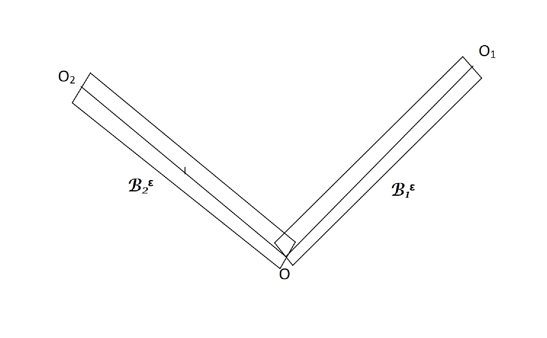
Let $e_{1},e_{2},\dots,e_{n}$ be $n$ closed segments in ${\mathbb{R}}^{2}$ , which have a single common point $O$ (i.e. the origin of the co-ordinate system), and let it be the common end point of all these segments. Let $\beta_{1},\beta_{2},\dots,\beta_{n}$ be $n$ bounded segments in ${\mathbb{R}}^{2}$ containing the point $O$ , the middle point of all segments, and such that $\beta_{j}$ is orthogonal to $e_{j}$ (for simplicity assume that the length $\left|\beta_{j}\right|$ of each $\beta_{j}$ is equal to 1). Let $\beta_{j}^{\varepsilon}$ be the image of $\beta_{j}$ obtained by a homothetic contraction in $\frac{1}{\varepsilon}$ times with the center $O$ . Denote ${\mathcal{B}}_{j}^{\varepsilon}$ the open rectangles with the bases $\beta_{j}^{\varepsilon}$ and with the heights $e_{j}$ , denote also $\hat{\beta_{j}^{\varepsilon}}$ the second base - side of each rectangle ${\mathcal{B}}_{j}^{\varepsilon}$ and let $O_{j}$ be the end of the segment $e_{j}$ which belongs to the base $\hat{\beta_{j}^{\varepsilon}}$ (see Fig. 4). Define the graph of the tube structure as the bundle of segments $e_{j}$ having a common point $O$ (see Fig. 3)

{\mathcal{B}}=\bigcup_{j=1}^{n}e_{j}.

Denote below $O_{0}=O$ . Let $\gamma_{j}^{\varepsilon}$ , $j=0,1,\dots,n$ , be the images of the bounded domains $\gamma_{j}$ (such that $\bar{\gamma}_{j}$ contains the end of the segment $O_{j}$ and is independent of $\varepsilon$ ) obtained by a homothetic contraction in $\frac{1}{\varepsilon}$ times with the center $O_{j}$ .

Define the tube structure associated with the bundle ${\mathcal{B}}$ as a bounded domain (see Fig. 5):

{\mathcal{B}}^{\varepsilon}=\left(\left(\bigcup_{j=1}^{n}\bar{\mathcal{B}}_{j}^{\varepsilon}\right)\bigcup\left(\bigcup_{j=1}^{n}\bar{\gamma}_{j}^{\varepsilon}\right)\right)^{\prime}

Here the prime stands for the set of the interior points. Assume that $\partial{\mathcal{B}}^{\varepsilon}\in C^{2}$ (the result may be generalized for the case of the piecewise smooth boundary $\partial{\mathcal{B}}^{\varepsilon}$ with no reentrant corners). Assume that the bases $\hat{\beta_{j}^{\varepsilon}}$ of ${\mathcal{B}}_{j}^{\varepsilon},$ $j=1,\dots,n$ , are some parts of $\partial{\mathcal{B}}^{\varepsilon}$ . We add the domains $\gamma_{j}^{\varepsilon}$ , $j=0,1,\dots,n$ , to smoothen the boundary of the tube structure.

Consider the following system of equations:

\left\{\begin{array}[c]{ll}-\mathrm{div}(\nu(x){\mathcal{D}}u_{\varepsilon})+\nabla p_{\varepsilon}=f(x)&\text{in }{\mathcal{B}}^{\varepsilon},\\ \mathrm{div}u_{\varepsilon}=0&\text{in }{\mathcal{B}}^{\varepsilon},\\ u_{\varepsilon}=g&\text{on }\partial{\mathcal{B}}^{\varepsilon}.\end{array}\right.

(28)

Here, $g=0$ on the lateral boundary of the rectangles composing ${\mathcal{B}}^{\varepsilon}$ ; moreover $g=0$ anywhere with the exception of the sides $\hat{\beta_{j}^{\varepsilon}}$ of the rectangles ${\mathcal{B}}_{j}^{\varepsilon}$ (these sides are assumed to belong to the boundary of the tube structure); $g\in C^{2}(\hat{\beta}_{j}^{\varepsilon})$ , and for each $j$ , $g=\varepsilon^{2}g_{j}(\frac{x-O_{j}}{\varepsilon})$ on $\hat{\beta_{j}^{\varepsilon}}$ , the vector valued functions $g_{j}\in C^{2}$ do not depend on $\varepsilon$ . Let $f$ be a vector-valued function of $(L^{2}({\mathcal{B}}^{\varepsilon}))^{2}$ . The solvability condition gives the relation

\int_{\partial{\mathcal{B}}^{\varepsilon}}g.n\mathrm{d}s=0.

(29)

Introduce the local system of coordinates $Ox_{1}^{e_{j}}x_{2}^{e_{j}}$ associated with the segment $e_{j}$ such that the direction of the axis $Ox_{1}^{e_{j}}$ coincides with the direction of the segment $OO_{j}$ , i.e. $x_{1}^{e_{j}}$ is the longitudinal coordinate. The axes $Ox_{1}^{e_{j}}x_{2}^{e_{j}}$ form a Cartesian coordinate system. Denote $d_{0}\varepsilon$ the infimum of radius of all circles with the center $O$ such that every point of it belongs only to not more than one of the rectangles ${\mathcal{B}}_{j}^{\varepsilon}$ , $j=1,\dots,n$ and $d_{1}$ is the maximal diameter of the domains $\gamma_{0},\gamma_{1},\dots,\gamma_{n}$ . We finally introduce the notation

\hat{d}_{0}\varepsilon=\max\{d_{0}\varepsilon,d_{1}\varepsilon\}.

Consider the right hand side vector valued function $f$ ”concentrated” in some neighborhoods of the nodes $O_{j}$ and diffused in the rectangles, i.e.

	$\displaystyle f$	$\displaystyle=\Phi_{j}\left(\frac{x-O_{j}}{\varepsilon}\right),$	$\displaystyle\text{for }\|x-O_{j}\|<\hat{d_{0}}\varepsilon,j=0,\dots,n,$		(30)
	$\displaystyle f$	$\displaystyle=f_{j}(x_{1}^{e_{j}}),$	$\displaystyle\text{for }\|x-O_{j}\|>\hat{d_{0}}\varepsilon,\ x_{1}^{e_{j}}\in(0,\|e_{j}\|),j=1,\dots,n.$		(30)

Here $f_{j}\in C_{0}^{\infty}([0,|e_{j}|]),\Phi_{j}\in C_{0}^{1}(Q)$ , $(j=0,1,\dots,n),$ where $Q$ is a ball $|\xi|<\hat{d_{0}}$ . Assume that

\nu(x)=\nu_{0}+\nu_{j}(x_{1}^{e_{j}})

(31)

such that $\nu_{j}(x_{1}^{e_{j}})=0$ for all $x_{1}^{e_{j}}\in[0,\beta]\cup[|e_{j}|-\beta;|e_{j}|]$ , where $\beta$ is a positive constant such that $\beta<min_{j}\frac{|e_{j}|}{4}$ ; $\nu\in C^{2}$ and there exist $\kappa_{0}\in{\mathbb{R}}^{+}$ such that $\nu(x)>\kappa_{0}$ for all $x\in{\mathcal{B}}^{\varepsilon}$ . Without loss of generality we may assume that $f_{j}\left(x_{1}^{e_{j}}\right)=0$ for all $x_{1}^{e_{j}}\in[0,\beta]\cup[|e_{j}|-\beta;|e_{j}|]$ .

Let $H_{\mathrm{div}=0}({\mathcal{B}}^{\varepsilon})$ be space of the divergence free vector valued functions from $H^{1}({\mathcal{B}}^{\varepsilon})$ . Let $H_{\mathrm{div}=0}^{0}({\mathcal{B}}^{\varepsilon})$ be the subspace of vector valued functions of $H_{\mathrm{div}=0}({\mathcal{B}}^{\varepsilon})$ vanishing at the boundary. Assume that $g$ can be continued in ${\mathcal{B}}^{\varepsilon}$ as a vector valued $\hat{g}$ of $H_{\mathrm{div}=0}({\mathcal{B}}^{\varepsilon})$ . The variational formulation for (28) is as follows: find $u_{\varepsilon}\in H_{\mathrm{div}=0}({\mathcal{B}}^{\varepsilon})$ such that $v_{\varepsilon}=u_{\varepsilon}-\hat{g}\in H_{\mathrm{div}=0}^{0}({\mathcal{B}}^{\varepsilon})$ , and such that it satisfies to the integral identity

\int_{{\mathcal{B}}^{\varepsilon}}\nu(x){\mathcal{D}}v_{\varepsilon}:{\mathcal{D}}{\varphi}=\int_{{\mathcal{B}}^{\varepsilon}}f\cdot\varphi-\int_{{\mathcal{B}}^{\varepsilon}}\nu(x){\mathcal{D}}\hat{g}:{\mathcal{D}}\varphi,\ \ \forall\varphi\in H_{\mathrm{div}=0}^{0}({\mathcal{B}}^{\varepsilon}).

The Riesz theorem will give the existence and the uniqueness of such a solution because the norms $\|v\|=\sqrt{\int_{{\mathcal{B}}^{\varepsilon}}\nu(x){\mathcal{D}}v:{\mathcal{D}}v}$ and $\|v\|_{(H^{1}({\mathcal{B}}^{\varepsilon}))^{2}}$ are equivalent. We have as a consequence that

\|v_{\varepsilon}\|_{(H^{1}({\mathcal{B}}^{\varepsilon}))^{2}}\leq{\mathcal{C}}(C_{PF},\kappa_{0})\left(\|f\|_{L^{2}({\mathcal{B}}^{\varepsilon})^{2}}+\|\hat{g}\|_{(H^{1}({\mathcal{B}}^{\varepsilon}))^{2}}\right),

where $C_{PF}$ is independent on $\varepsilon$ (see [10]) and $\kappa_{0}$ is the lower bound of the viscosity (31)..

Proposition 3.1.

If $u_{\varepsilon}$ is a weak solution for problem (28) then there exists a distribution $p_{\varepsilon}\in{{\mathcal{D}}}^{{}^{\prime}}({\mathcal{B}}^{\varepsilon})$ such that $(u_{\varepsilon},p_{\varepsilon})$ satisfies $\eqref{1}_{1}$ in the sense of distributions. The following inequality holds in the case of $\hat{g}=0$ :

\|\nabla p_{\varepsilon}\|_{H^{-1}(B^{\varepsilon})}\leq C\|f\|_{\left(L^{2}(B^{\varepsilon})\right)^{2}}.

Here $C$ is a constant independent of $\varepsilon.$

The proof is similar to that of the Propositions of section 2.

3.1 Asymptotic expansion

We construct the main part of the asymptotic expansion in a form

u^{a}=\displaystyle{\sum_{l=0}^{k}\varepsilon^{l+2}\left\{\sum_{e=e_{j};j=1,\dots,n}u_{l}^{e}(x^{e,L})\chi_{\varepsilon}(x)+\sum_{i=0}^{n}u_{l}^{BLO_{i}}\left(\frac{x-O_{i}}{\varepsilon}\right)\right\}}

(32)

\begin{array}[c]{lcl}p^{a}&=&\displaystyle{\sum_{l=0}^{k}\varepsilon^{l+1}\left\{\sum_{e=e_{j};j=1,\dots,n}p_{l}^{e}(x^{e,L})\chi_{\varepsilon}(x)+\sum_{i=0}^{n}p_{l}^{BLO_{i}}\left(\frac{x-O_{i}}{\varepsilon}\right)\right\}}+\\ &&+\displaystyle{\sum_{e=e_{j};j=1,\dots,n}\sum_{l=0}^{k}\varepsilon^{l}q_{l}^{e}(x_{1}^{e})\chi_{\varepsilon}(x)+\sum_{i=0}^{n}q_{0}^{e_{i}}(x_{1}^{e_{i}}=0)\left(1-\chi_{\varepsilon}(x)\right)\theta_{i}(x)}\end{array}

(33)

$x^{e,L}=(x_{1}^{e},\frac{x_{2}^{e}}{\varepsilon})$ . Later, in the end of the section we will add an exponentially small corrector multiplying the boundary layers by a cut-off function $\eta$ in the subdomain where the boundary layers are just exponentially small (see (42), (43)). The last sum in (28) is taken for all nodes $O_{i}$ and the value $q_{0}^{e_{i}}(x_{1}^{e_{i}}=0)$ is calculated at the point $x=O_{i}$ ; function $q_{0}^{e_{i}}$ is supposed to be continuous on the graph ${\mathcal{B}}$ . Here $\chi_{\varepsilon}(x)$ is a function equal to zero at the distance less than $(\hat{d_{0}}+1)\varepsilon$ from $O_{j}$ , $j=0,1,\dots,n$ , equal to zero on the rectangle ${\mathcal{B}}_{j}^{\varepsilon}$ if $x_{1}^{e_{j}}\leq(\hat{d_{0}}+1)\varepsilon$ or if $|x_{1}^{e_{j}}-|e_{j}||\leq(\hat{d_{0}}+1)\varepsilon$ ; we suppose that function $\chi_{\varepsilon}$ is equal to one on this rectangle if $x_{1}^{e_{j}}\geq(\hat{d_{0}}+2)\varepsilon$ and $|x_{1}^{e_{j}}-|e_{j}||\geq(\hat{d_{0}}+2)\varepsilon$ , and we define $\chi_{\varepsilon}$ by the relations $\chi_{\varepsilon}(x)=\chi\left(\frac{x_{1}^{e_{j}}}{\varepsilon}\right)$ if $(\hat{d_{0}}+1)\varepsilon\leq x_{1}^{e_{j}}\leq(\hat{d_{0}}+2)\varepsilon$ and $\chi_{\varepsilon}(x)=\chi\left(\frac{x_{1}^{e_{j}}-|e_{j}|}{\varepsilon}\right)$ if $(\hat{d_{0}}+1)\varepsilon\leq|e_{j}|-x_{1}^{e_{j}}\leq(\hat{d_{0}}+2)\varepsilon$ . Here $\chi$ is a differentiable on ${\mathbb{R}}$ function of one variable, it is independent of $\varepsilon$ , it is equal to zero on the segment $[-(\hat{d_{0}}+1);(\hat{d_{0}}+1)]$ and it is equal to one on the union of intervals $(-\infty,-(\hat{d_{0}}+2))\cup((\hat{d_{0}}+2),+\infty)$ . Moreover $\chi_{\varepsilon}$ is equal to zero on every $\gamma_{j}^{\varepsilon}$ . The functions ${\theta_{i}}$ , $i=1,...,n,$ are defined as follows

	$\displaystyle\theta_{j}=0$	$\displaystyle\|x-O_{j}\|>min_{i}\frac{\|e_{i}\|}{2}$
	$\displaystyle\theta_{j}=1$	$\displaystyle\|x-O_{j}\|\leq min_{i}\frac{\|e_{i}\|}{2}$

The relation between the vector-columns $x^{T}$ and $x^{e_{j},T}$ (here $T$ is the transposition symbol) is given by

x^{T}=\Gamma_{j}x^{e_{j},T}+O\qquad j=1,\dots,n

where $\Gamma_{j}$ is an orthogonal matrix of passage from the canonic base to the local one. Then applying the results of section 2, for every channel ${\mathcal{B}}_{j}^{\varepsilon},$ we get $u_{l}^{e}$ , $p_{l}^{e}$ and $q_{l}^{e}$ defined up to the scalar constants $c_{l}^{e}$ , $d_{l}^{e}$ . Indeed, denote $\hat{q}_{l}^{e_{j}}(x_{1}^{e_{j}})$ the solution of equation (11) with $\dfrac{\partial\hat{q}_{l}^{e_{j}}}{\partial x_{1}^{e_{j}}}(0)=0.$ Then the general solution of equation (11) has a form:

q_{l}^{e_{j}}(x_{1}^{e_{j}})=\hat{q}_{l}^{e_{j}}(x_{1}^{e_{j}})+c_{l}^{e_{j}}\int_{0}^{x_{1}^{e_{j}}}\nu(s)\mathrm{d}s+d_{l}^{e_{j}},

(34)

where $c_{l}^{e_{j}}$ and $d_{l}^{e_{j}}$ are the undetermined constants;

u_{l}^{e_{j}}(x^{e_{j},L})=\Gamma_{j}\left(\tilde{u}_{l}^{e_{j}}(x^{e_{j},L})\right)^{T},

where the second component of $\tilde{u}_{l}^{e_{j}}$ does not depend on $c_{l}^{e_{j}}$ , $d_{l}^{e_{j}}$ (see (10)₂); the same property holds for $p_{l}^{e_{j}}$ (see (10)₃); the first component $\tilde{u}_{1,l}^{e_{j}}$ (see (10)₁) depends on $c_{l}^{e_{j}}$ :

	$\displaystyle\tilde{u}_{1,l}^{e_{j}}$	$\displaystyle=-D^{-2}\left\{\frac{\partial^{2}\tilde{u}_{2,l-2}^{e_{j}}}{\partial\xi_{2}^{e_{j}}\partial x_{1}^{e_{j}}}+\frac{2}{\nu(x_{1}^{e_{j}})}\left(\frac{\partial}{\partial x_{1}^{e_{j}}}\left(\nu(x_{1}^{e_{j}})\frac{\partial\tilde{u}_{1,l-2}^{e_{j}}}{\partial x_{1}^{e_{j}}}\right)-\frac{\partial p_{l-1}^{e_{j}}}{\partial x_{1}^{e_{j}}}\right)\right\}+$
		$\displaystyle+\frac{2}{\nu(x_{1}^{e_{j}})}N_{1}(\xi_{2}^{e_{j}})\left(\frac{\partial\hat{q}_{l}^{e_{j}}}{\partial x_{1}^{e_{j}}}-f_{1}\delta_{j0}\right)+2c_{l}^{e_{j}}N_{1}(\xi_{2}^{e_{j}})$
		$\displaystyle=\hat{u}_{1,l}^{e_{j}}+2c_{l}^{e_{j}}N_{1}(\xi_{2}^{e_{j}}).$

For $x_{1}^{e_{j}}\in[0,{\beta}]\bigcup[|e_{j}|-{\beta},|e_{j}|]$ , $\hat{u}_{l}^{e_{j}}$ , $\tilde{p}_{l}^{e_{j}}$ and $\partial\hat{q}_{l}^{e_{j}}/\partial x_{1}^{e_{j}}$ may be taken equal to zero because the right hand side $f_{j}$ is equal to zero for this values of $x_{1}^{e_{j}}$ , while the flow rate $\int_{\beta_{j}}\tilde{u}_{1,l}^{e_{j}}(\xi_{2}^{e_{j}})d\xi_{2}^{e_{j}}$ is constant on $e_{j}$ . $N_{1}$ is the function introduced in section 2.

To get the problems for the boundary layers, we introduce the domain $\Omega_{O_{0}}=\displaystyle{\cup_{j=1}^{n}\tilde{\Omega}_{j}\cup\gamma_{0}}$ , where $\tilde{\Omega}_{j}$ are the half-infinite strips obtained from ${\mathcal{B}}_{j}^{\varepsilon}$ by infinite extension behind the base $\tilde{\beta}_{j}^{\varepsilon}$ and by homothetic dilatation in $\frac{1}{\varepsilon}$ times (with respect to the point $O$ ); let $\Omega_{j}$ be obtained from $\tilde{\Omega}_{j}$ by a symmetric reflection relatively to the line containing $\beta_{j}^{\varepsilon}$ and let $\Omega_{O_{j}}=\tilde{\Omega}_{j}\cup\gamma_{j}^{t}$ , where $\gamma_{j}^{t}$ is obtained from $\gamma_{j}$ by a translation (such that the point $O_{j}$ becomes $O$ ).

Since $\nu(x)=\nu_{0}$ for all $x_{1}^{e_{j}}\in[0,\beta]\cup[|e_{j}|-\beta;|e_{j}|]$ , the boundary layer solution is a pair constituted of a vector valued function $u_{l}^{BLO_{j}}$ and a scalar function $p_{l}^{BLO_{j}}$ satisfying to the Stokes system:

\left\{\begin{array}[c]{l}-\frac{\nu_{0}}{2}\Delta_{\xi}u_{l}^{BLO_{0}}+\nabla_{\xi}p_{l}^{BLO_{0}}=\Phi_{0}(\xi)\delta_{l,0}+\\ \ \ \ +\displaystyle{\sum_{e=e_{j};j=1,\dots,n}}\left\{c_{l}^{e}\left(\nu_{0}\Delta_{\xi}\left(\chi_{j}(\xi_{1}^{e})\Gamma_{j}\left(N_{1}(\xi_{2}^{e}),0\right)^{T}\right)-\nabla_{\xi}\left(\chi_{j}(\xi_{1}^{e})\xi_{1}^{e}\right)\right)-d_{l+1}^{e}\nabla_{\xi}\chi_{j}(\xi_{1}^{e})\right\},\\ \\ \mathrm{div}_{\xi}u_{l}^{BLO_{0}}=-\displaystyle{\sum_{e=e_{j};\ j=1,\dots,n}}\mathrm{div}_{\xi}\left(c_{l}^{e}\left(\chi_{j}(\xi_{1}^{e})\Gamma_{j}\left(N_{1}(\xi_{2}^{e}),0\right)^{T}\right)\right),\text{ \ \ if }\xi\in\Omega_{O_{0}},\\ {u_{l}^{BLO_{0}}}{|_{\partial\Omega_{O_{0}}}}=0,\end{array}\right.

(35)

and for $j=1,\dots,n,$

\left\{\begin{array}[c]{l}-\frac{\nu_{0}}{2}\Delta_{\hat{\xi}}u_{l}^{BLO_{j}}+\nabla_{\hat{\xi}}p_{l}^{BLO_{j}}=\\ \ \ \ =\Phi_{j}(\hat{\xi})\delta_{l,0}+\hat{c}_{l}^{e}\left(\nu_{0}\Delta_{\hat{\xi}}\left(\chi_{j}(\hat{\xi}_{1}^{e})\right)\hat{\Gamma}_{j}\left(N_{1}(\hat{\xi}_{2}^{e}),0\right)^{T}-\nabla_{\hat{\xi}}\left(\chi_{j}(\hat{\xi}_{1}^{e})\hat{\xi}_{1}^{e}\right)\right)-\hat{d}_{l+1}^{e}\nabla_{\hat{\xi}}\chi_{j}(\hat{\xi}_{1}^{e}),\\ \\ \mathrm{div}_{\hat{\xi}}u_{l}^{BLO_{j}}=-\hat{c}_{l}^{e_{j}}\mathrm{div}_{\hat{\xi}}\left(\chi_{j}(\hat{\xi}_{1}^{e_{j}})\hat{\Gamma}_{j}\left(N_{1}(\hat{\xi}_{2}),0\right)^{T}\right),\text{ \ \ if }\hat{\xi}\in\Omega_{O_{j}},\\ {u_{l}^{BLO_{j}}}_{|_{\partial\Omega_{O_{j}},\hat{\xi}_{1}^{e_{j}}=0}}=g_{j}\delta_{l,0},\\ {u_{l}^{BLO_{j}}}_{|_{\partial\Omega_{O_{j}},\hat{\xi}_{1}^{e_{j}}\neq 0}}=0.\end{array}\right.

(36)

The variable $\hat{\xi}_{1}^{e_{j}}$ is opposite to $\xi_{1}^{e_{j}}$ , i.e. to the first component of the vector $\Gamma_{j}^{T}\xi^{T}$ . So $\hat{\xi}_{1}^{e_{j}}=\hat{\Gamma}_{j}^{T}\xi^{T}$ , where $\hat{\Gamma}_{j}=\hat{I}d\Gamma_{j}$ and $\hat{I}d$ is the diagonal matrix with the diagonal elements $-1,1$ . The constants $\hat{c}_{l}^{e_{j}}$ , $\hat{d}_{l}^{e_{j}}$ are defined in such a way that the functions $c_{l}^{e_{j}}\int_{0}^{x_{1}^{e_{j}}}\nu(s)\mathrm{d}s+d_{l}^{e_{j}}$ and $\hat{c}_{l}^{e_{j}}\int_{0}^{|e_{j}|-x_{1}^{e_{j}}}\nu(s)\mathrm{d}s+\hat{d}_{l}^{e_{j}}$ are equal, i.e.

c_{l}^{e_{j}}=-\hat{c}_{l}^{e_{j}},\ \ \ \hat{d}_{l}^{e_{j}}=c_{l}^{e_{j}}\int_{0}^{|e_{j}|}\nu(s)\mathrm{d}s+d_{l}^{e_{j}}.

(37)

Assume that every term in the sum $\displaystyle{\sum_{e=e_{j};j=1,\dots,n}}$ in (35) is defined only in the branch of $\Omega_{O_{0}}$ , corresponding to $e=e_{j}$ , and it vanishes in $\gamma_{0}$ .

The solutions of these boundary layer problems decay exponentially at infinity and the constants $c_{l}^{e_{j}}$ , $\hat{c}_{l}^{e_{j}}$ , ${d}_{l}^{e_{j}}$ and $\hat{d}_{l}^{e_{j}}$ are chosen from the conditions of existence of such solutions (see [8]). Let us define first $\hat{c}_{l}^{e_{j}}$ from the condition of exponential decaying of $u_{l}^{BLO_{j}}$ at infinity:

\int_{\Omega_{O_{j}}}\hat{c}_{l}^{e_{j}}\mathrm{div}_{\hat{\xi}}\left(\chi_{j}(\hat{\xi}_{1}^{e_{j}})\hat{\Gamma}_{j}\left(N_{1}({\xi}_{2}^{e}),0\right)^{T}\right)d\hat{\xi}=\int_{\beta_{j}}\left(\hat{\Gamma}_{j}^{T}g_{j}\right)^{1}\mathrm{d}{\xi}_{2}^{e}\delta_{l,0},

i.e.

-\int_{\beta_{j}}N_{1}(\xi_{2}^{e_{j}})\mathrm{d}{\xi}_{2}^{e}\hat{c}_{l}^{e_{j}}=\int_{\beta_{j}}\left(\hat{\Gamma}_{j}^{T}g_{j}\right)^{1}\mathrm{d}{\xi}_{2}^{e}\delta_{l,0},

(38)

where the upper index $1$ corresponds to the first component of the vector.

Then we find $\hat{c}_{l}^{e_{j}}$ , and $\hat{d}_{l}^{e_{j}}$ as defined in (37). Then we determine the constants ${d}_{l+1}^{e_{j}}$ from the condition of the exponential decaying of $p_{l}^{BLO_{0}}$ at infinity. To this end, consider first problem (35) without the last term in equation ${\eqref{8}}_{1}$ , i.e.

\left\{\begin{array}[c]{l}-\frac{\nu_{0}}{2}\Delta_{\xi}\bar{u}_{l}^{BLO_{0}}+\nabla_{\xi}\bar{p}_{l}^{BLO_{0}}=\\ \ \ \ \ =\Phi_{0}(\xi)\delta_{l,0}+\displaystyle{\sum_{e=e_{j};j=1,\dots,n}}\left\{c_{l}^{e}\left(\nu_{0}\Delta_{\xi}\left(\chi_{j}(\xi_{1}^{e})\right)\Gamma_{j}\left(N_{1}(\xi_{2}^{e}),0\right)^{T}-\nabla_{\xi}\left(\chi_{j}(\xi_{1}^{e})\xi_{1}^{e}\right)\right)\right\},\\ \\ \mathrm{div}_{\xi}\bar{u}_{l}^{BLO_{0}}=-\displaystyle{\sum_{e=e_{j};j=1,\dots,n}}\mathrm{div}_{\xi}c_{l}^{e}\left(\chi_{j}(\xi_{1}^{e})\Gamma_{j}\left(N_{1}(\xi_{2}^{e}),0\right)^{T}\right),\quad\xi\in\Omega_{O_{0}},\\ \\ {\bar{u}_{l}^{BLO_{0}}}{|_{\partial{\Omega}_{O_{0}}}}=0.\end{array}\right.

(39)

Here the constants $c_{l}^{e_{j}}$ are just defined by (37) and (38) and satisfy the condition

\int_{\Omega_{O_{0}}}{\sum_{e=e_{j};\ j=1,\dots,n}}\mathrm{div}_{\xi}c_{l}^{e}\left(\chi_{j}(\xi_{1}^{e})\Gamma_{j}\left(N_{1}({\xi}_{2}^{e}),0\right)^{T}\right)d{\xi}_{2}^{e}=0

i.e.

{\sum_{e=e_{j};j=0,1,\dots,n}}\int_{\beta_{j}}c_{l}^{e_{j}}N_{1}(\xi_{2}^{e})d{\xi}_{2}^{e}=0.

(40)

Indeed, the choice of constants $c_{l}^{e_{j}}=-\hat{c}_{l}^{e_{j}}$ and $c_{l}^{e_{j}}$ from (38) and condition (29) give relation (40).

It is known that there exists the unique solution $\{\bar{u}_{l}^{BLO_{0}},\bar{p}_{l}^{BLO_{0}}\}$ of this problem such that $\bar{u}_{l}^{BLO_{0}}$ stabilizes to zero at infinity on every branch of $\Omega_{0}$ and $\bar{p}_{l}^{BLO_{0}}$ stabilizes on every branch of $\Omega_{0}$ associated to $e_{j}$ , to its own constant $\bar{p}_{l}^{BLO_{0}\infty j}$ . These constants are defined uniquely up to one common additive constant, which we fix here by a condition $\bar{p}_{l}^{BLO_{0}\infty 1}=0$ . Then we define

\left\{\begin{array}[c]{l}{d}_{l+1}^{e_{j}}=-\bar{p}_{l}^{BLO_{0}\infty j},\\ \\ u_{l}^{BLO_{0}}=\bar{u}_{l}^{BLO_{0}},\\ \\ {p}_{l}^{BLO_{0}}=\bar{p}_{l}^{BLO_{0}}+\displaystyle{\sum_{e=e_{j};j=1,\dots,n}}{d}_{l+1}^{e_{j}}\chi_{j}(\xi_{1}^{e_{j}})\end{array}\right.

(41)

on every branch of $\Omega_{0}$ , associated with $e_{j}$ , i.e. ${p}_{l}^{BLO_{0}}=\bar{p}_{l}^{BLO_{0}}-{\sum_{e=e_{j};j=1,\dots,n}}\bar{p}_{l}^{BLO_{0}\infty j}\chi_{j}.$

Obviously, this pair $\{{u}_{l}^{BLO_{0}},{p}_{l}^{BLO_{0}}\}$ satisfies (35). The boundary layer functions ${u}_{l}^{BLO_{j}}$ and ${p}_{l}^{BLO_{j}}$ ; $j=0,1,\dots,n$ are not defined in the vicinity of $O$ . Therefore we should change a little bit the formulas of $u^{a}$ and $p^{a}$ far from the nodes $O_{j}$ , $j=0,1,\dots,n$ .

Let $\eta_{j}(x_{1}^{e_{j}})$ be a smooth function defined on each segment $e_{j}$ , let it be one if $\left|x_{1}^{e_{j}}-\frac{|e_{j}|}{2}\right|\geq\frac{|e_{j}|}{2}-\beta$ and let it be zero if $\left|x_{1}^{e_{j}}-\frac{|e_{j}|}{2}\right|\leq\frac{|e_{j}|}{8}$ . Let $\eta(x)=\eta_{j}(x_{1}^{e_{j}})$ for each rectangle ${\mathcal{B}}_{j}^{\varepsilon}$ and let $\eta=1$ on each $\gamma_{j}^{\varepsilon}$ . Set $\eta^{(j)}(x)=\eta(x)$ on $\gamma_{j}^{\varepsilon}$ and all half-rectangles having common points with $\gamma_{j}^{\varepsilon}$ and extend it by zero on the remaining part of ${\mathcal{B}}_{j}^{\varepsilon}$ . Then we define $u^{a}$ and $p^{a}$ as

\bar{u}^{a}=\displaystyle{\sum_{l=0}^{k}\varepsilon^{l+2}\left\{\sum_{e=e_{j};j=0,1,\dots,n}u_{l}^{e}(x^{e,L})\chi_{\varepsilon}(x)+\sum_{i=0}^{n}u_{l}^{BLO_{i}}\left(\frac{x-O_{i}}{\varepsilon}\right)\eta^{(i)}(x)\right\},}

(42)

\begin{array}[c]{lcl}\bar{p}^{a}&=&\displaystyle{\sum_{l=0}^{k}\varepsilon^{l+1}\left\{\sum_{e=e_{j};j=0,1,\dots,n}p_{l}^{e}(x^{e,L})\chi_{\varepsilon}(x)+\sum_{i=0}^{n}p_{l}^{BLO_{i}}\left(\frac{x-O_{i}}{\varepsilon}\right)\eta^{(i)}(x)\right\}}\\ &&+\displaystyle{\sum_{l=0}^{k}\varepsilon^{l}q_{l}^{e}(x_{1}^{e})\chi_{\varepsilon}(x)+\sum_{i=0}^{n}q_{0}^{e_{i}}(x_{1}^{e_{i}}=0)\left(1-\chi_{\varepsilon}(x)\right)\theta_{i}(x).}\end{array}

(43)

Let us mention that the last term (sum) in (43) corresponds to the boundary layer function $p_{l}^{BLO_{j}}$ for $l=-1.$

3.2 Error estimate

In this section we estimate the error between the exact solution and the asymptotic one. Substituting the asymptotic expansions (42), (43), into (28), we get the relations

\left\{\begin{array}[c]{ll}-\mathrm{div}(\nu(x){\mathcal{D}}\bar{u}^{a})+\nabla\bar{p}^{a}=f(x)&\\ \ \ \ \ \ \ -\displaystyle{\sum_{e=e_{j};j=1,\dots,n}}\left\{{\varepsilon}^{k+1}\Gamma_{j}\left(F_{e_{j}}^{k}\right)^{T}\chi_{\varepsilon}(x)-\varepsilon^{k}(\nabla_{\xi}\chi_{j}(\xi_{1}^{e_{j}})d_{k+1}^{e_{j}}\right.&\\ \qquad\qquad\left.-\nabla_{\tilde{\xi}}\chi_{j}(\tilde{\xi}_{1}^{e_{j}}){d}_{k+1}^{e_{j}})\right\}+\Psi,&\text{in }{\mathcal{B}}^{\varepsilon},\\ \mathrm{div}\bar{u}^{a}=\psi&\text{in }{\mathcal{B}}^{\varepsilon},\\ \bar{u}^{a}=g&\text{on }\partial{\mathcal{B}}^{\varepsilon},\end{array}\right.

(44)

where $F_{e_{j}}^{k}$ is the residual described in (15), and $\psi$ is defined by

\psi(x,t)=\left\{\begin{array}[c]{ll}\displaystyle 0&\mathrm{in}~{\mathcal{B}}^{\varepsilon}\cap\left\{x^{e_{i}}_{1}<\beta\right\},\\ \displaystyle-\nabla_{x}\eta_{i}(x_{1}^{e_{i}}).u^{(BLO_{0})}\left(\frac{x-O_{0}}{\varepsilon}\right)&\mathrm{in}~{\mathcal{B}}^{\varepsilon}\cap\left\{\beta<x_{1}^{e_{i}}<\frac{3|e_{i}|}{8}\right\},\\ 0&\mathrm{in}~{\mathcal{B}}^{\varepsilon}\cap\left\{\frac{3|e_{i}|}{8}<x_{1}^{e_{i}}<\frac{5|e_{i}|}{8}\right\},\\ \displaystyle-\nabla_{x}\eta_{i}(x_{1}^{e_{i}}).u^{(BLO_{i})}\left(\frac{x-O_{i}}{\varepsilon}\right)&\mathrm{in}~{\mathcal{B}}^{\varepsilon}\cap\left\{\frac{5|e_{i}|}{8}<x_{1}^{e_{i}}<|e_{i}|\right\},\\ 0&\mathrm{in}~\gamma_{i}^{\varepsilon},i=1,\dots,n,\\ &\end{array}\right.

(45)

$\|\Psi\|_{\left(L^{2}(({\mathcal{B}}^{\varepsilon})\right)^{2}}=O\left(\exp(\frac{-c}{\varepsilon})\right)$ , $\|\psi\|_{H^{1}({\mathcal{B}}^{\varepsilon})}=O\left(\exp(\frac{-c}{\varepsilon})\right)$ with a positive constant $c$ and ${\displaystyle\int_{{\mathcal{B}}^{\varepsilon}}}\psi\mathrm{d}s=0,$ because $\displaystyle{\int_{\partial{\mathcal{B}}^{\varepsilon}}(\bar{u}^{a},n)\mathrm{d}s=\int_{\partial{\mathcal{B}}^{\varepsilon}}(g,n)\mathrm{d}s=0}$ . The exponentially decaying residuals $\Psi$ and $\psi$ appear from the truncation of the boundary layer terms by the function $\eta$ : it is different from 1 in the part of the domain ${\mathcal{B}}^{\varepsilon}$ where $u_{l}^{BLO_{i}}\left(\frac{x-O_{i}}{\varepsilon}\right)$ , $p_{l}^{BLO_{i}}\left(\frac{x-O_{i}}{\varepsilon}\right)$ and their derivatives are exponentially small. We are going to prove the estimate

\|u-\bar{u}^{a}\|_{H^{1}({\mathcal{B}}^{\varepsilon})}=O\left({{\varepsilon}^{k+\frac{1}{2}}}\right).

We can not apply directly the a priori estimates because $\bar{u}^{a}$ is not divergence free.
Let us construct a function $\hat{U}^{a}:{\mathcal{B}}^{\varepsilon}\rightarrow{\mathbb{R}}^{2}$ satisfying the following properties:

\left\{\begin{array}[c]{ll}\displaystyle\hat{U}^{a}\in\left(H_{0}^{1}({\mathcal{B}}^{\varepsilon})\right)^{2},&\\ \displaystyle\mathrm{div}_{x}\hat{U}^{a}=\psi&\mathrm{in}\qquad{\mathcal{B}}^{\varepsilon},\\ \hat{U}^{a}=0&\mathrm{in}\quad{\mathcal{B}}^{\varepsilon}\cap\{x^{e}_{1}<\hat{d}_{0}\varepsilon\}\bigcup\gamma_{j}^{\varepsilon},j=1,\dots,n\\ &\end{array}\right.

(46)

Proposition 3.2.

Problem (46) has at least one solution, satisfying

\|\hat{U}^{a}\|_{(H^{1}({\mathcal{B}}^{\varepsilon}))^{2}}=O(exp(-c/\varepsilon))

Proof. Due to (46)₃ we can consider the problem (46) as separate problem on each ${\mathcal{B}}^{\varepsilon}_{j}$ . Denote by $\hat{U}^{e_{j}}$ the restriction of $\hat{U}^{a}$ on ${\mathcal{B}}^{\varepsilon}_{j}$ , obviously $\hat{U}^{e_{j}}(x_{1}^{e_{j}},x_{2}^{e_{j}})=0$ for $(x\in{\mathcal{B}}^{\varepsilon}_{j}$ such that $x_{1}^{e_{j}}<\hat{d}_{0}\varepsilon$ . For all $(x\in{\mathcal{B}}^{\varepsilon}_{j}$ such that $x_{1}^{e_{j}}>\hat{d}_{0}\varepsilon$ introduce the new variable $(y_{1}^{e_{j}},y_{2}^{e_{j}})=\left(\frac{x_{1}^{e_{j}}-\hat{d}_{0}\varepsilon}{|e_{j}|-\hat{d}_{0}\varepsilon},\frac{x_{2}^{e_{j}}}{\varepsilon}\right)$ ; obviously $(y_{1}^{e_{j}},y_{2}^{e_{j}})\in(0,1)\times(-\frac{1}{2},\frac{1}{2})$ . Define a new function $\mu_{\varepsilon}^{e_{j}}:(0,1)\times(-\frac{1}{2},\frac{1}{2})\longrightarrow{\mathbb{R}}^{2}$ , by $\mu_{\varepsilon}^{e_{j}}(y_{1}^{e_{j}},y_{2}^{e_{j}})=\left(\frac{1}{|e_{j}|-\hat{d}_{0}\varepsilon}\hat{U}_{1}^{e_{j}}((|e_{j}|-\hat{d}_{0}\varepsilon)y_{1}^{e_{j}}+\hat{d}_{0}\varepsilon,\varepsilon y_{2}^{e_{j}}),\frac{1}{\varepsilon}\hat{U}_{2}^{e_{j}}((|e_{j}|-\hat{d}_{0}\varepsilon)y_{1}^{e_{j}}+\hat{d}_{0}\varepsilon,\varepsilon y_{2}^{e_{j}})\right)$ . Obvious computations lead to the following problem for $\mu_{\varepsilon}^{e_{j}}$ :

\left\{\begin{array}[c]{ll}\displaystyle\mathrm{div}_{y}\mu_{\varepsilon}^{e_{j}}=\psi((|e_{j}|-\hat{d}_{0}\varepsilon)y_{1}^{e_{j}}+\hat{d}_{0}\varepsilon,\varepsilon y_{2}^{e_{j}})&\mathrm{in}\qquad(0,1)\times(-\frac{1}{2},\frac{1}{2}),\\ \mu_{\varepsilon}^{e_{j}}=0&\mathrm{on}\qquad\partial((0,1)\times(-\frac{1}{2},\frac{1}{2})),\\ &\end{array}\right.

(47)

Applying the result of [4], Chap. III, p. 127 we get: there exist a solution of 47) such that

\|\mu_{\varepsilon}^{e_{j}}\|_{\left(H^{1}((0,1)\times(-\frac{1}{2},\frac{1}{2}))\right)^{2}}=O(exp(-c/\varepsilon)).

(48)

Expressing the norm of $\hat{U}^{e_{j}}$ with respect to the norm $\mu_{\varepsilon}^{e_{j}}$ we obtain

\|\hat{U}^{e_{j}}\|_{\left(H^{1}({\mathcal{B}}^{\varepsilon}_{j}\cap\{x_{1}^{e_{j}}<\hat{d}_{0}\varepsilon\})\right)^{2}}\leq\frac{1}{\varepsilon^{\frac{1}{2}}}\|\mu_{\varepsilon}^{e_{j}}\|_{\left(H^{1}((0,1)\times(-\frac{1}{2},\frac{1}{2}))\right)^{2}},

i.e. $\|\hat{U}^{e_{j}}\|_{\left(H^{1}({\mathcal{B}}^{\varepsilon}_{j}\cap\{x_{1}^{e_{j}}<\hat{d}_{0}\varepsilon\})\right)^{2}}=O(exp(-c/\varepsilon))$ . So, $\|\hat{U}^{a}\|_{(H^{1}({\mathcal{B}}^{\varepsilon}))^{2}}=O(exp(-c/\varepsilon))$ .

Define $U^{a}=\bar{u}^{a}-\hat{U}^{a}$ . Then $\left(U^{a},\bar{p}^{a}\right)$ satisfies the following problem :

\left\{\begin{array}[c]{ll}-\mathrm{div}(\nu(x){\mathcal{D}}U^{a})+\nabla\bar{p}^{a}=f(x)+\mathrm{div}(\nu(x){\mathcal{D}}\hat{U}^{a})+\Psi&\\ -\displaystyle{\sum_{e=e_{j};j=1,\dots,n}}\left\{{\varepsilon}^{k+1}\Gamma_{j}\left(F_{e_{j}}^{k}\right)^{T}\chi_{\varepsilon}(x)-\varepsilon^{k}(\nabla_{\xi}\chi_{j}(\xi_{1}^{e_{j}})d_{k+1}^{e_{j}}-\nabla_{\tilde{\xi}}\chi_{j}(\tilde{\xi}_{1}^{e_{j}})\tilde{d}_{k+1}^{e_{j}})\right\},&\text{in }{\mathcal{B}}^{\varepsilon},\\ \mathrm{div}\bar{u}^{a}=0&\text{in }{\mathcal{B}}^{\varepsilon},\\ \bar{u}^{a}=g&\text{on }\partial{\mathcal{B}}^{\varepsilon},\end{array}\right.

(49)

Theorem 3.1.

Let $(\bar{u}^{a},\bar{p}^{a})$ be the asymptotic solution given by (42), (43) and $(u_{\varepsilon},p_{\varepsilon})$ the solution of (28), the following estimates hold:

\left\{\begin{array}[c]{l}\|\bar{u}^{a}-u_{\varepsilon}\|_{{H^{1}({\mathcal{B}}^{\varepsilon})}^{2}}=O\left(\varepsilon^{k+\frac{1}{2}}\right),\\ \|\nabla\bar{p}^{a}-\nabla p_{\varepsilon}\|_{{H^{1}({\mathcal{B}}^{\varepsilon})}}=O\left(\varepsilon^{k+\frac{1}{2}}\right).\end{array}\right.

(50)

Applying a priori estimates and (48) we get

\|U^{a}-u_{\varepsilon}\|_{H^{1}({\mathcal{B}}^{\varepsilon})}=O\left(\varepsilon^{k+\frac{1}{2}}\right)

and so,

\|\bar{u}^{a}-u_{\varepsilon}\|_{H^{1}({\mathcal{B}}^{\varepsilon})}=O\left(\varepsilon^{k+\frac{1}{2}}\right)

The estimate for the pressure is obtained from the a priori estimates. These estimates justify the construction of the asymptotic expansion.

Remark 3.1.

The main result can be easily generalized in case when the length of $\beta_{j}$ is different from 1.

Remark 3.2.

Formula (38) shows that only $c^{e_{j}}_{0}$ could be different from zero. The same analysis can be provided in the case of a multi-bundle structure, that is the union of a finite number of thin domains of ${\mathcal{B}}^{\varepsilon}$ type (see [10], section 4.5.2), and in this case the constants $c^{e_{j}}_{l}$ should be determined from a system of linear algebraic equations (see (4.5.43),(4.5.44) in [10]).

4 Numerical experiments

1. We consider the Stokes flow in a rectangular domain $(0,1)\times(0,\varepsilon)$ with $\varepsilon=0.1$ :

\left\{\begin{array}[c]{ll}\displaystyle-\mathrm{div}(\nu(x_{1})Du)+\nabla p=0&\displaystyle\text{ in }(0,1)\times(0,\varepsilon)\\ \displaystyle\mathrm{div}u=0&\displaystyle\text{ in }(0,1)\times(0,\varepsilon)\\ \displaystyle u(0,x_{2})=\varepsilon^{2}\frac{x_{2}}{\varepsilon}\left(1-\frac{x_{2}}{\varepsilon}\right)&\displaystyle\text{ on }(0,\varepsilon)\\ &\\ \displaystyle u(1,x_{2})=\varepsilon^{2}\frac{x_{2}}{\varepsilon}\left(1-\frac{x_{2}}{\varepsilon}\right)&\displaystyle\text{ on }(0,\varepsilon)\\ \displaystyle u(x_{1},0)=u(x_{1},\varepsilon)&\displaystyle\text{ on }(0,1)\end{array}\right.

(51)

here $\nu(x_{1})=2x_{1}+2$ . From (10) we get for $j=0$ :

\left\{\begin{array}[c]{l}\displaystyle\frac{\partial}{\partial x_{1}}\left(\frac{1}{\nu(x_{1})}\frac{\partial q_{0}}{\partial x_{1}}\right)=0\\ \\ \displaystyle u_{0,1}=\varepsilon^{2}\frac{1}{\nu(x_{1})}\frac{\partial q_{0}}{\partial x_{1}}\frac{x_{2}}{\varepsilon}\left(1-\frac{x_{2}}{\varepsilon}\right)\\ \displaystyle u_{0,2}=0\\ \displaystyle p_{0}=0\end{array}\right.

with the compatibility condition (20) we have :

\int_{0}^{1}\xi_{2}(1-\xi_{2})-u_{0,1}(0,\xi_{2})\mathrm{d}\xi_{2}=0

Since we assume that $p(1,x_{2})=0$ we get :

\left\{\begin{array}[c]{l}\displaystyle q_{0}(x_{1})=-x_{1}(x_{1}+2)+3\\ \\ \displaystyle u_{0,1}=\varepsilon^{2}\frac{x_{2}}{\varepsilon}\left(1-\frac{x_{2}}{\varepsilon}\right)\\ u_{0,2}=0\\ p_{0}=0\end{array}\right.

Solving numerically the problem (51) (by Comsol) we get the following results : for the first component of the velocity we have :

and for the pressure :

The error between the numerical result and the leading term of the asymptotic expansion is as follows :

We see that the error is of order of $\varepsilon$ et $\varepsilon^{5}$ for the pressure and the velocity respectively.

2. Consider now the Stokes problem (51) in a T-shape domain ${\mathcal{B}}^{\varepsilon}=(-1,0]\times(0,\varepsilon)\cup(0,\varepsilon)\times(-0.45,0.55)$

\left\{\begin{array}[c]{ll}\displaystyle u(1,x_{2})=g_{1}\left(\frac{x_{2}}{\varepsilon}\right)=\varepsilon^{2}\frac{x_{2}}{\varepsilon}\left(1-\frac{x_{2}}{\varepsilon}\right)&\text{ on }(0,\varepsilon)\\ &\\ \displaystyle u(x_{1},-0.45)=g_{2}\left(\frac{x_{1}}{\varepsilon}\right)=\varepsilon^{2}\frac{x_{1}}{\varepsilon}\left(1-\frac{x_{1}}{\varepsilon}\right)&\text{ on }(0,\varepsilon)\\ &\\ \displaystyle u(x_{1},-0.45)=g_{3}\left(\frac{x_{1}}{\varepsilon}\right)=2\varepsilon^{2}\frac{x_{1}}{\varepsilon}\left(1-\frac{x_{1}}{\varepsilon}\right)&\text{ on }(0,\varepsilon)\\ &\\ &\end{array}\right.

(52)

as inflow/outflow conditions, $\varepsilon=0.1$ , $u=0$ anywhere else on the boundary and $\displaystyle\nu(x_{1},x_{2})=2+2(x_{1}+1)\mu_{1}(x_{1})+2(x_{2}+1)\mu_{2}(x_{2})+2(x_{2}+1)\mu_{3}(x_{2})$ . $\mu_{i}$ are defined in such a way that $\nu$ is equal to $2x_{1}^{e_{j}}+2$ in each rectangle and constant near the nodes. The functions $\mu_{1},\mu_{2}$ and $\mu_{3}$ have the following shape :

So we get

We do two crop sections, the first in ${\mathcal{B}}_{2}^{\varepsilon}=(0,\varepsilon)\times(0,0.55)$ and the second in ${\mathcal{B}}_{3}^{\varepsilon}=(0,\varepsilon)\times(-0.45,0)$ , and the results are as follows :

We see that the error is of order of $\varepsilon^{5}$ as in the case of a rectangle and estimates. It confirms the theoretical prediction in section3.

Acknowledgments. The authors were partially supported by the following grants: ”Strutture sottili” of the program ”Collaborazioni interuniversitarie internazionali” (2004-2006) of the Italian Ministry of Education, University and Research; SFR MOMAD of the university of Saint Etienne and ENISE ( the Ministry of the Research and Education of France), the joint French-Russian PICS CNRS grant ”Mathematical modeling of blood diseases” and by the grant no. 14.740.11.0875 ”Multiscale problems: analysis and methods” of the Ministry of Edication and Research of Russian Federation.

References

[1] Blanc F., Gipouloux O., Panasenko G., Zine A.M., Asymptotic analysis and partial asymptotic decomposition of the domain for Stokes equation in tube structure, Mathematical Models and Methods in Applied Sciences, 1999, Vol.9, 9, 1351-1378.
[2] Cardone G., Corbo Esposito A., Panasenko G.P., Asymptotic partial decomposition for diffusion with sorption in thin structures, Nonlinear Analysis 65, 2006, 79-106.
[3] Cardone G., Panasenko G.P., Sirakov Y., Asymptotic analysis and numerical modeling of mass transport in tubular structures, Mathematical Models and Methods in Applied Sciences (M3AS) 20, n. 4 (2010) 1-25.
[4] Galdi G.P., An introduction to the Mathematical Theory of the Navier-Stokes Equations, Springer-Verlag, New York, 1994.
[5] Girault V., Raviart P.A., Finite Element Methods for Navier-Stokes Equations, Springer-Verlag, Berlin,1986.
[6] B.M.Haine,I.S. Aranson,L. Berlyand and D.A.Karpeev, Effective viscosity of dilute bacterial suspensions: Atwo dimensional problem, Physi.Biol.,5 (2008),1-9.
[7] Ladyzhenskaya O.A., The Mathematical Theory of Viscous Incompressible Flow, Gordon and Breach Sc. Publ, New York, 1969.
[8] Nazarov S.A., Plamenevskii B.A., Elliptic Problems in Domains with Piecewise Smooth Boundaries, Berlin-New York: Walter de Gruyter, 1994.
[9] Panasenko G.P., Asymptotic expansion of the solution of Navier-Stokes equation in a tube structure, C.R.Acad.Sci.Paris, t. 326, Série IIb, 1998, pp. 867-872.
[10] Panasenko G.P., Multi-scale Modeling for Structures and Composites, Springer, Dordrecht, 2005.