Strongly anisotropic non-equilibrium phase transition in Ising models with friction
Abstract
The non-equilibrium phase transition in driven two-dimensional Ising models with two different geometries is investigated using Monte Carlo methods as well as analytical calculations. The models show dissipation through fluctuation induced friction near the critical point. We first consider high driving velocities and demonstrate that both systems are in the same universality class and undergo a strongly anisotropic non-equilibrium phase transition, with anisotropy exponent . Within a field theoretical ansatz the simulation results are confirmed. The crossover from Ising to mean field behavior in dependency of system size and driving velocity is analyzed using crossover scaling. It turns out that for all finite velocities the phase transition becomes strongly anisotropic in the thermodynamic limit.
pacs
05.70.Ln, 68.35.Af, 05.50.+q, 05.70.FhI Introduction
The interest in magnetic contributions to friction due to spin correlations has strongly increased in recent years. One interesting aspect is the energy dissipation due to the formation of spin waves in a two-dimensional Heisenberg model induced by a moving magnetic tip [1, 2, 3], which can be of Stokes or Coulomb type depending on the intrinsic relaxation time scales [4]. On the other hand, magnetic friction occurs also in bulk systems moving relative to each other. Kadau et al. [5] used a two-dimensional Ising model, cut into two halves parallel to one axis and moved along this cut with the velocity , to explore surface friction. The motion drives the system out of equilibrium into a steady state, leading to a permanent energy flux from the surface to the heat bath. This model exhibits a non-equilibrium phase transition, which has been investigated in several different geometries [6] by means of analytical treatment as well as Monte Carlo (MC) simulations. The critical temperature of the considered models depends on the velocity and has been calculated exactly for various geometries in the limit . In this limit the class of models show mean field-like critical behavior. Subsequent investigations have been done in a variety of context, in particular for driven Potts models [7] and for rotating Ising chains of finite length [8].
The nature of non-equilibrium phase transitions is still a field of large interest, and simple models helping to explore this field are seldom. A very famous example is the driven lattice gas (DLG) [9, 10, 11], exhibiting a strongly anisotropic phase transition. Despite a lot of similarities between the driven lattice gas and the Ising model with friction, there is an important difference: The order parameter is conserved in the former, while it is non-conserved in the latter model. A further class of models characterized by non-equilibrium phase transitions are sheared systems [12, 13, 14], experimentally accessible within the framework of binary liquid mixtures.
Like the driven lattice gas, the systems investigated in the following exhibit a strongly anisotropic phase transition, which is investigated by means of Monte Carlo simulations as well as a field theoretical ansatz.In addition, the case of finite velocities is analyzed by means of crossover scaling, where a broad range of velocities and system sizes are analysed. We show that for all the considered models end up in the mean field class with strongly anisotropic correlations as soon as the system size exceeds a velocity dependent crossover length .
While a crossover behavior from Ising to mean field class occurs in various thermodynamic systems such as ionic fluid [15, 16] and spin systems with long-range interactions [17], to our knowledge such a crossover including a change from isotropic to strongly anisotropic behavior has not been investigated in detail until now. The paper is organized as follows: After introducing the model and geometries, we determine the anisotropy exponent for using MC simulations as well as a field theoretical model. Then we turn to finite velocities and present the crossover scaling analysis. Finally we discuss our results.
II Models
The systems considered in this work are denoted 2d and 1+1d and are shown in Fig. 1 (for a classification see [6]). The 2d system is a two-dimensional two-layer Ising model with lattice sites, where the two layers are moved relative to each other along the parallel direction. Each lattice site carries one spin variable , and only nearest-neighbor interactions are taken into account. Periodic boundary conditions are applied in both planar directions, i.e., . In order to simulate a finite velocity using Monte Carlo simulations the upper sub-system is moved times by one lattice constant during each random sequential Monte Carlo sweep (MCS). Since one MCS corresponds to the typical time a spin needs to relax into the direction of its local Weiss field, and as the lattice constant is of the order , the velocity is given in natural units .
Instead of moving the two layers against each other, we reorder the couplings between the subsystems with time to simplify the implementation [6]. Introducing a time-dependent displacement
| (1) |
which is increased by one after each random sequential spin flip attempts, the Hamiltonian can be expressed as
| (2) |
with the reduced nearest neighbor coupling , the reduced boundary coupling , and . In the following we assume .
The critical temperature of the regarded systems increases with and saturates for high velocities. In the limit an analytical calculation of the critical temperature for the 2d geometry yield
| (3) |
for [6]. The basic idea of the analytic solution provides the approach for the implementation of infinite velocity, which works as follows: the interaction partner for a spin in the lower layer is chosen randomly from the same row in the upper layer. Thus we can use Eq. (2) with a random value .
The 1+1d system consists of a two-dimensional Ising model, where all rows are moved relative to each other. The displacement as well as the coupling is equal for all adjacent rows, leading to the Hamiltonian
| (4) |
Again, periodic boundary conditions are applied in both directions, where discontinuities in direction are avoided through the homogeneous displacement [6]. The analytical treatment at gave the critical temperature
| (5) |
for in this case [6]. Within the scope of the 1+1d model the velocity corresponds to a shear rate, which is ofter denoted as [18, 19]. However, we will use the term velocity for both driving mechanisms throughout this work.
In the following we argue that both systems show the same underlying critical behavior. In order to emphasize the similarity, Fig. 2 illustrates slight variations of both models. First of all we start with the 1+1d model (a) and change every second bond perpendicular to the motion into a stationary bond. Additionally, we perform a transformation that changes the homogeneous shear into an alternating shift of the double chains and reverses () every second double chain, leading to the configuration in Fig. 2b. These modifications do not change the critical behavior of the 1+1d system, since still one-dimensional chains (now consisting of two rows) are moved relative to each other. On the other hand, the cross section of the 2d model can be visualized in a slightly different way (see Fig. 2d) without altering the corresponding Hamiltonian, Eq. (2). Since the next nearest double chains in (b) are not moving relative to each other, the only difference between (b) and (d) are the third nearest neighbor bonds in (d), which are irrelevant at the critical point where long range correlations dominate. Hence we conclude that both systems belong to the same universality class.
III Results
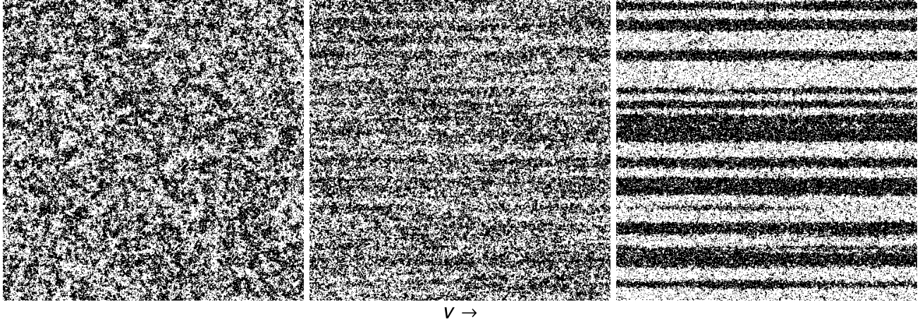
In order to illustrate symptomatic features of both systems, Fig. 3 shows a sequence of spin configurations of one layer of the d system (note that the same characteristics are observed in the 1+1d system). On the left hand side an equilibrated system at well above the critical temperature of the non-moving system, [20], is presented. Shortly after starting the motion stripe-like domains arise, spanning the whole system parallel to the motion. The stripes are rather stable, but are nonetheless transient, since they grow in time until the system ends up in a homogeneously magnetized state. The evolution in Fig. 3 is an example for a velocity driven phase transition already described in [5, 6], which is triggered by the onset of the motion and the associated increase of the critical temperature. The circumstances are comparable to a quench, which is characterized by a temperature decrease below . After a quench a coarsening of domains is observed, whereas the growth of the domains can be described by a power law (e.g. [21, 22]). Domain growth in systems exhibiting a strongly anisotropic phase transition, e.g., the DLG model, is also a well investigated subject [23, 10, 24]. The corresponding time evolution of spin configurations are similar to those shown in Fig. 3, leading to the assumption that the 2d and the 1+1d geometries are also characterized by strongly anisotropic correlations, which is shown in the following section.
III.1 Determination of in the limit
A strongly anisotropic phase transition is characterized by a correlation length which diverges with direction dependent critical exponents at the critical point 11 1 Throughout this work, the symbol means “asymptotically equal” in the respective limit, e. g., Note that the variable is used for the reduced temperature throughout the rest of this work.,
| (7) |
with direction and reduced critical temperature . Defining the anisotropy exponent [26, 27, 28]
| (8) |
we find
| (9) |
independent of . Isotropic scaling takes place for and strongly anisotropic scaling is implied by . Several models with strongly anisotropic behavior where studied in the past. Examples are Lifshitz points as present in the anisotropic next nearest neighbor Ising (ANNNI) model [29, 30], the non-equilibrium phase transition in the DLG [10], the two-dimensional dipolar in-plane Ising-model [28]. Furthermore, strongly anisotropic behavior usually occurs in dynamical systems, where the parallel direction can be identified with time and the perpendicular direction(s) with space [27, 31]. In the latter case the anisotropy exponent corresponds to the dynamical exponent .
The knowledge of the anisotropy exponent is essential and necessary for appropriate simulations of strongly anisotropic systems. To avoid complicated shape effects it is required to keep the generalized aspect ratio [26, 27, 28]
| (10) |
fixed, which requires the knowledge of . We will show in the following that the limit simplifies the analysis for infinite velocity and turns out to be essential at finite .
We first discuss the case and always assume criticality, . In order to determine the anisotropy exponent we calculate the perpendicular correlation function between spins at distance in cylinder geometry (leading to ), and thereby gain the correlation length through
| (11) |
where the prefactor is shown to be proportional to in Appendix A. Approaching the critical point within the given geometry, the correlation length is limited by , and using Eq. (9) this leads to the relation
| (12) |
with non-universal amplitude [32, 28]. Measuring the correlation length in dependency of the parallel extension allows us to determine the anisotropy exponent .
In the simulations, the limit is implemented by the condition . This is sufficient to keep the sytematic errors in smaller than the statistical error adequate to calculate . From we can determine the required system sizes via , where the factor 2 accounts for the periodic boundary conditions. As for and for for the 1+1d model (see Fig. 4(left)) we yield for and for meaning that for large systems a much smaller value of would be sufficient.
Fig. 4 displays the correlation functions for both models. For the 1+1d case these correlations are purely exponential also at short distances, since the coupling in direction is mediated through fluctuating fields [6], leading to dimensional reduction to an effectively one-dimensional system. The resulting correlation length is shown in the inset of Fig. 4(left). The growth of follows a power law with exponent and with prefactor
| (13) |
indicated as a black line.
In the case of the 2d model (right figure in Fig.4) we find two regions with different characteristics. The short-distance correlations are affected by the nearest-neighbor interactions within the planes which are not present in the 1+1d model. These correlations decay with a correlation length of the order . For large distances the correlations crossover to an exponential behavior. The exponential correlations are propagated by the fluctuations of stripe-like domains. The analysis yields
| (14) |
in this case.
From the anisotropy exponent we can derive the correlation length exponents and using the generalized hyper-scaling relation
| (15) |
with and mean field exponents , , and , whose validity has been demonstated in [6] by a mapping onto a mean field equilibrium model.
The calculatation of in the limit is done within a one-dimensional Ginzburg-Landau-Wilson (GLW) field theory [33]. For it was shown in Ref. [6] that the 1+1d model can be mapped onto an equilibrium system consisting of one-dimensional chains that only couple via fluctuating magnetic fields. Due to the stripe geometry with short length and the periodic boundary conditions in direction the magnetization is homogeneous in direction, and parallel correlations are irrelevant. Hence we can use the zero mode approximation in this direction. However, it is necessary to include a term representing the interaction between adjacent spin chains. This can be expressed by the square of the spatial derivative of the magnetization in the direction to the motion. Hence the minimal GLW model to describe this strongly anisotropic mean field system is given by
| (16) |
with phenomenological parameters and , where represents the magnetization of the spin chain at coordinate . Eq. (16) corresponds to the Hamiltonian used for the description of a cylinder-like spin system, which is infinite along one dimension, and finite and periodic in dimensions [33]. The partition function of Eq. (16) can be mapped onto a one-dimensional Schrödinger equation in a quartic anharmonic oscillator potential using a rescalation, which yields the critical exponents and . The detailed derivation is given in Appendix A.
III.2 Crossover scaling at finite velocities
We now turn to finite velocities. The following analysis is exemplarily done for the 1+1d model, but as stated above, both models belong to the same universality class and similar results are expected for the 2d model. As we expect a crossover from an isotropic Ising model with to a strongly anisotropic system with , we must be careful with the system geometry: We cannot use a fixed finite generalized aspect ratio , Eq. (10), in the simulations, as is not constant. The only possible choice is (or ), where the -dependency drops out.
We consider the correlation length at reduced critical temperature
| (17) |
where . is calculated via a finite-size scaling analysis of the perpendicular correlation length (not shown). As this procedure becomes inaccurate for small velocities , we calculate the critical temperature according to
| (18) |
with in these cases, where we assume in agreement with the literature [10, 18, 19]. The results are shown in the inset of Fig. 5a.
Fig. 5a shows the unscaled data, which gives evidence that the correlation length of systems moved at high velocities are well described by the exponent (dotted line), whereas for low velocities effectively the Ising exponent (dashed line) holds for the simulated system sizes . The curvature of the data of intermediate velocities suggest the crossover. As a data collapse on the analytical known [34] relation (dashed line in Fig. 5) has to be obtained in the limit , both axes must be rescaled by the same factor . This crossover length can be determined by applying the following method: We start with plotting the correlation length in the mean field limit . Then we subsequently add the data for smaller by rescaling and with , which shifts the points parallel to the dashed line, until a data collapse is obtained (see Fig. 5b). This procedure works quite accurate for velocities , only at very small the errors in grow due to the fact that we just shift the data along the dashed line. The resulting crossover length is pictured as black dots in the inset of Fig. 5a. The behavior of is analogous to the velocity dependency of other quantities like the critical temperature or the energy dissipation, which are characterized by a power law for and a saturation for .
We conclude that for all finite velocities the critical behavior changes from Ising type to mean field type at a velocity dependent crossover length approximately given by
| (19) |
(solid red curve in the inset of Fig. 5a), where the velocity is measured in units and the size in . The velocity independent prefactor was added to shift the crossover point, i.e., the intersection of the asymptotes, to . The saturation of at results from the lattice cut-off, as . The inset in Fig. 5b shows the effective exponent , obtained from the logarithmic derivative
| (20) |
whose value changes from (Ising, isotropic) to (MF, strongly anisotropic). Note that we verified the mean field exponents for with finite-size scaling methods and also found good agreement of the scaling function with the universal finite-size scaling function [35](not shown). In order to illustrate the change of the critical behavior, Fig. 6 shows typical critical spin configurations for different values of the crossover scaling variable .
We are now able to compare our results with the literature. If the crossover scaling variable Ising-like behavior occurs, whereas for mean field exponents and strongly anisotropic correlations are expected. In experiments [13], even slow shear rates of the order of (in natural units , where now is the time scale of the fluid dynamics), lead to a crossover length and, as the typical system size is large wrt. the atomic distances, give , indicating that experimental data are always obtained in the mean field limit.
In relation to the results of Winter et al. [19] we find that the correlation length exponent has been measured in the regime , leading to the anisotropy exponent in agreement with our results. In Ref. [18] the correlation length exponents have also been determined in the mean field limit. Looking at the lowest velocity we find , where a surprisingly small anisotropy exponent has been estimated. The highest velocity leads to and . These discrepancies might be attributed to the fact that an integral quantity, the order parameter, has been measured, as well as to strong surface effects induced by the open boundary conditions used in the direction.
IV Conclusion

In this work we investigated two recently proposed driven Ising models with friction due to magnetic interactions, namely the 1+1d and 2d model, using MC simulations as well as analytical methods. At first we focused on the strongly anisotropic critical behavior and calculated the anisotropy exponent in the limit of high driving velocity . Therefore the perpendicular correlation function of a cylinder-like geometry was calculated at criticality for different system sizes. Evaluating the connection between system size and correlation length, Eq. (12), we were able to find the critical exponents as well as and . The analytic deviation of these exponents within the framework of a Ginzburg-Landau-Wilson Hamiltonian led to the same values. Comparing the results to the driven lattice gas [9, 10] we note that it also shows a strongly anisotropic phase transition at a critical temperature which grows with the velocity. Remarkably this phase transition is characterized by the same critical exponents at large fields.
Finally we focused on the critical behavior for finite velocities and performed extensive MC simulations in order to calculate the crossover scaling function describing the crossover from the Ising universality class at to the non-equilibrium critical behavior at . The analysis has exemplarily been done for the 1+1d model, but as shown, both models belong to the same universality class and similar results are expected for the 2d model. In the analysis an additional complexity arised due to the strongly anisotropic characteristics of the correlations. Therefore we calculated the correlation length in a cylindrical system, circumventing intricate shape effects. We were able to identify a crossover length using a simple method based on the rescaling of data for each velocity such that a data collapse occurs. This procedure leads to an excellent data collapse of all simulation results for different velocities and system sizes .
It turns out that for all finite velocities the models undergo a crossover, at crossover length , from an quasi-equilibrium isotropic Ising-like phase transition to a non-equilibrium mean-field behavior with strongly anisotropic correlations.
Acknowledgements.
We thank Felix M. Schmidt and Matthias Burgsmüller for valuable discussions. This work was supported by CAPES–DAAD through the PROBRAL program as well as by the German Research Society (DFG) through SFB 616 “Energy Dissipation at Surfaces”.Appendix A Scaling exponents of the GLW model
The following calculation is similar to [33]. Discretizing the integral
| (21) |
with step size , , and gives
| (22) |
In order to evaluate the partition function
| (23) |
we use abbreviations in analogy to transfer matrices,
| (24) |
with to get
| (25) | |||||
for the assumed periodic boundary conditions.
Let and be the result of the integrations for the interval . Since is near-diagonal for , we can write as
| (26) |
where denotes the growth factor of the integrations corresponding to the leading eigenvalue of the transfer matrix . The integral over in the partition function becomes
| (27) | |||||
and yields the solution of the integrations for the interval . Hence we get a differential equation for ,
| (28) |
We now substitute
| (29a) | |||||
| (29b) | |||||
| (29c) | |||||
| (29d) | |||||
and expand to lowest order around to yield the Schrödinger equation in a quartic potential,
| (30) |
valid in the scaling limit , with kept fixed.
The correlation length is determined from the lowest eigenvalues of this equation, as
| (31) |
From the substitution, Eqs. (29), we directly read off the exponents , and .
References
- [1] C. Fusco, D. E. Wolf, and U. Nowak, Phys. Rev. B 77, 174426 (2008).
- [2] M. P. Magiera, L. Brendel, D. E. Wolf, and U. Nowak, EPL 87, 26002 (2009a).
- [3] M. P. Magiera, D. E. Wolf, L. Brendel, and U. Nowak, IEEE Trans. Mag. 45, 3938 (2009b).
- [4] M. P. Magiera, S. Angst, A. Hucht, and D. E. Wolf, Phys. Rev. B 84, 212301 (2011).
- [5] D. Kadau, A. Hucht, and D. E. Wolf, Phys. Rev. Lett. 101, 137205 (2008).
- [6] A. Hucht, Phys. Rev. E 80, 061138 (2009).
- [7] F. Igloi, M. Pleimling, and L. Turban, Phys. Rev. E 83, 041110 (2011).
- [8] H. J. Hilhorst, J. Stat. Mech. Theor. Exp. , P04009 (2011).
- [9] S. Katz, J. L. Lebowitz, and H. Spohn, Phys. Rev. B 28, 1655 (1983).
- [10] B. Schmittmann and R. K. P. Zia, in Phase Transitions and Critical Phenomena, Vol. 17, edited by C. Domb and J. L. Lebowitz (Academic Press, London, 1995).
- [11] R. K. P. Zia, J. Stat. Phys 138, 20 (2010).
- [12] C. K. Chan and L. Lin, EPL 11, 13 (1990).
- [13] A. Onuki, J. Phys. Cond. Mat. 9, 6119 (1997).
- [14] E. N. M. Cirillo, G. Gonnella, and G. P. Saracco, Phys. Rev. E 72, 026139 (2005).
- [15] M. E. Fisher, J. Stat. Phys. 75, 1 (1994).
- [16] K. Gutkowski, M. A. Anisimov, and J. V. Sengers, J. Chem. Phys. 114, 3133 (2001).
- [17] E. Luijten, H. W. J. Blöte, and K. Binder, Phys. Rev. E 56, 6540 (1997).
- [18] G. P. Saracco and G. Gonnella, Phys. Rev. E 80, 051126 (2009).
- [19] D. Winter, P. Virnau, J. Horbach, and K. Binder, EPL 91, 60002 (2010).
- [20] A. Lipowski and M. Suzuki, Physica A 198, 227 (1993).
- [21] A. J. Bray, Adv. Phys 43, 357 (1994).
- [22] R. Paul, S. Puri, and H. Rieger, EPL 68, 881 (2004).
- [23] C. Yeung, T. Rogers, A. Hernandez-Machado, and D. Jasnow, J. Stat. Phys. 66, 1071 (1992).
- [24] P. I. Hurtado, J. Marro, and E. V. Albano, EPL 59, 14 (2002).
- [25] Throughout this work, the symbol means “asymptotically equal” in the respective limit, e.g., Note that the variable is used for the reduced temperature throughout the rest of this work.
- [26] K. Binder, in Finite Size Scaling and Numerical Simulations of Statistical Systems, edited by V. Privman (World Scientific, 1990) Chap. 4.
- [27] M. Henkel, Conformal Invariance and Critical Phenomena (Springer-Verlag, 1999).
- [28] A. Hucht, J. Phys A: Math. Gen. 35, L481 (2002).
- [29] W. Selke, Physics Reports 170, 213 (1988).
- [30] M. Pleimling and M. Henkel, Phys. Rev. Lett. 87, 125702 (2001).
- [31] H. Hinrichsen, Advances in Physics 49, 815 (2000).
- [32] M. Henkel and U. Schollwock, J. Phys A: Math. Gen. 34, 3333 (2001).
- [33] E. Brézin and J. Zinn-Justin, Nuclear Physics B 257, 687 (1985).
- [34] J. L. Cardy, J. Phys A: Math. Gen. 17, L385 (1984).
- [35] D. Grüneberg and A. Hucht, Phys Rev E 69, 036104 (2004).