Feature Selection via Regularized Trees
Abstract
We propose a tree regularization framework, which enables many tree models to perform feature selection efficiently. The key idea of the regularization framework is to penalize selecting a new feature for splitting when its gain (e.g. information gain) is similar to the features used in previous splits. The regularization framework is applied on random forest and boosted trees here, and can be easily applied to other tree models. Experimental studies show that the regularized trees can select high-quality feature subsets with regard to both strong and weak classifiers. Because tree models can naturally deal with categorical and numerical variables, missing values, different scales between variables, interactions and nonlinearities etc., the tree regularization framework provides an effective and efficient feature selection solution for many practical problems.
Index Terms:
regularized boosted trees; RBoost; regularized random forest; RRF; tree regularization.I Introduction
In supervised learning, given a training data set consisting of instances, predictor variables and the target variable , feature selection is commonly used to select a compact feature subset without significant loss of the predictive information about . Feature selection methods play an important role in defying the curse of dimensionality, improving efficiency both in time and space, and facilitating interpretability [1].
We propose a tree regularization framework for feature selection in decision trees. The regularization framework avoids selecting a new feature for splitting the data in a tree node when that feature produces a similar gain (e.g. information gain) to features already selected, and thus produces a compact feature subset. The regularization framework only requires a single model to be built, and can be easily added to a wide range of tree-based models which use one feature for splitting data at a node. We implemented the regularization framework on random forest (RF) [2] and boosted trees [3]. Experiments demonstrate the effectiveness and efficiency of the two regularized tree ensembles. As tree models naturally handle categorical and numerical variables, missing values, different scales between variables, interactions and nonlinearities etc., the tree regularization framework provides an effective and efficient feature selection solution for many practical problems.
Section II describes related work and background. Section III presents the relationship between decision trees and the Max-Dependency scheme [4]. Section IV proposes the tree regularization framework, the regularized random forest (RRF) and the regularized boosted random trees (RBoost). Section V establishes the evaluation criteria for feature selection. Section VI demonstrates the effectiveness and efficiency of RRF and RBoost by extensive experiments. Section VII concludes this work.
II Related Work and Background
II-A Related work
Feature selection methods can be divided into filters, wrappers and embedded methods [5]. Filters select features based on criteria independent of any supervised learner [6, 7]. Therefore, the performance of filters may not be optimum for a chosen learner. Wrappers use a learner as a black box to evaluate the relative usefulness of a feature subset [8]. Wrappers search the best feature subset for a given supervised learner, however, wrappers tend to be computationally expensive [9].
Instead of treating a learner as a black box, embedded methods select features using the information obtained from training a learner. A well-known example is SVM-RFE (support vector machine based on recursive feature elimination) [10]. At each iteration, SVM-RFE eliminates the feature with the smallest weight obtained from a trained SVM. The RFE framework can be extended to classifiers able to provide variable importance scores, e.g. tree-based models [11]. Also, decision trees such as C4.5 [12] are often used as embedded methods as they intrinsically perform feature selection at each node. Single tree models were used for feature selection [13], however, the quality of the selected features may be limited because the accuracy of a single tree model may be limited. In contrast, tree ensembles, consisting of multiple trees are believed to be significantly more accurate than a single tree [2]. However, the features extracted from a tree ensemble are usually more redundant than a single tree. Recently, [14] proposed ACE (artificial contrasts with ensembles) to select a feature subset from tree ensembles. ACE selects a set of relevant features using a random forest [2], then eliminates redundant features using the surrogate concept [15]. Also multiple iterations are used to uncover features of secondary effects.
The wrappers and embedded methods introduced above require building multiple models, e.g. the RFE framework [10] requires building potentially models. Even at the expense of some acceptable loss in prediction performance, it is very desirable to develop feature selection methods that only require training a single model which may considerably reduce the training time [5]. The tree regularization framework proposed here enables many types of decision tree models to perform feature subset selection by building the models only one time. Since tree models are popularly used for data mining, the tree regularization framework provides an effective and efficient solution for many practical problems.


II-B Information-theoretic measures and issues
Information-theoretic measures have been widely used for feature selection [16, 17, 7, 6, 4]. Entropy is an important concept in the information-theoretic criteria. The entropy of a categorical variable can be expressed in terms of prior probabilities: . The entropy of after observing another categorical variable is: . The increase in the amount of information about after observing is called the mutual information or, alternatively, information gain [6]:
| (1) |
is symmetric, i.e. , and models the degree of association between and . Therefore, one can use to evaluate the relevancy of for predicting the class , and use to evaluate the redundancy in a pair of predictor variables [4]. In addition, a measure called symmetric uncertainty: is used in feature selection methods such as CFS (correlation-based feature selection) [6] and FCBF (fast correlation-based filter) [7].
Measures like and capture only two-way relationships between variables and can not capture the relationship between two variables given other variables, e.g. [16, 17]. [17] illustrated this limitation using an exclusive OR example: , in which neither nor individually is predictive, but and together can correctly determine . To this end, [16, 17] proposed measures which can capture three-way interactions. Still, a feature selection method capable of handling -way interactions when is desirable [16]. However, it is computationally expensive to do so [17].
II-C Tree-based models and issues
Univariate decision trees such as C4.5 [12] or CART [15] recursively split data into subsets. For many tree models, the feature used for splitting in a node is selected to optimize an information-theoretic measure such as information gain.
A tree model is able to capture multi-way interactions between the splitting variables and potentially is a solution for the issue of the information-theoretic measures mentioned in Section II-B. However, tree models have their own problems for selecting a non-redundant feature set. A decision tree selects a feature at each node by optimizing, commonly, an information-theoretic criterion and does not consider if the feature is redundant to the features selected in previous splits, which results in feature redundancy. The feature redundancy problem in tree models is illustrated in Figure 1. For the two-class data shown in the figure, after splitting on (“split 1”), either or can separate the two classes (“split 2”). Therefore is the minimal feature set that can separate the two-class data. However, a decision tree may use for “split 1” and for “split 2” and thus introduce feature redundancy.
The redundancy problem becomes even more severe in tree ensembles which consist of multiple trees. To eliminate the feature redundancy in a tree model, some regularization is used here to penalize selecting a new feature similar to the ones selected in previous splits.

III Relationship between decision trees and the Max-Dependency scheme
The conditional mutual information, that is, the mutual information between two features and given a set of other features , …, is defined as
| (2) |
where is the ratio of the number of instances satisfying to the total number of instances.
A first-order incremental feature selection scheme, referred to as the Max-Dependency (MD)[4] scheme, is defined as
| (3) |
where is the step number, is the feature set selected in the first steps (), is the index of the feature selected at each step, is the mutual information between and given the feature set .
Here we consider the relationship between the MD scheme and decision trees. Because Equation (2) is limited to categorical variables, the analysis in this section is limited to categorical variables. We also assume the decision trees discussed in this section select the splitting variable by maximizing the information gain and split a non-leaf node into child nodes, where is the number of values of the splitting variable. However the tree regularization framework introduced later is not limited to such assumptions.
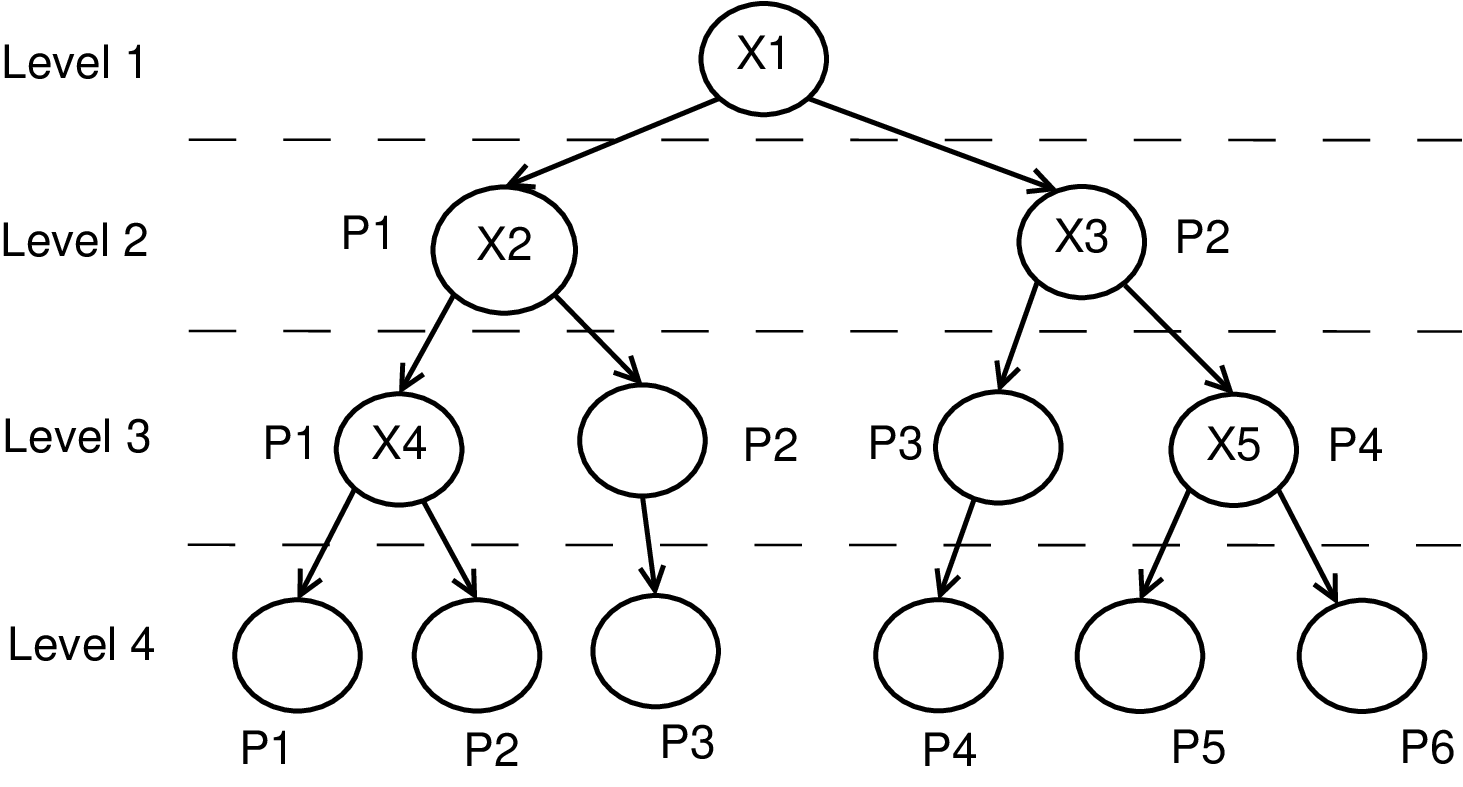
In a decision tree, a node can be located by its level (depth) and its position in that level. An example of a decision tree is shown in Figure 2(a). The tree has four levels, and one to six nodes (positions) at each level. Note that in the figure, a tree node that is not split is not a leaf node. Instead, we let all the instances in the node pass to its “imaginary” child node, to keep a form similar to the MD tree structure introduced later.
Also, let denote the set of feature-value pairs that define the path from the root node to node . For example, for node P6 at level 4 in Figure 2(a), . For a decision tree node , a variable is selected to maximize the information gain conditioned on . That is,
| (4) |
By viewing each step of the MD scheme as a level in a decision tree, the MD scheme can be expressed as a tree structure, referred to an MD tree. An example of an MD tree is shown in Figure 2(b). Note in an MD tree, only one feature is selected at each level. Furthermore, for the MD tree, is selected at so that
| (5) |
where is the ratio of the number of instances at node to the total number of training instances.
Note Equation (4) maximizes the conditional mutual information at each node, while Equation (5) maximizes a weighted sum of the conditional mutual information from all the nodes in the same level. Calculating Equation (5) is more computationally expensive than Equation (4). However, at each level , an MD tree selects only one feature that adds the maximum non-redundant information to the selected features, while decision trees can select multiple features and there is no constraint on the redundancy of these features.
IV Regularized trees
We are now in a position to introduce the tree regularization framework which can be applied to many tree models which recursively split data based on a single feature at each node. Let be the evaluation measure calculated for feature . Without loss of generality, assume the splitting feature at a tree node is selected by maximizing (e.g. information gain). Let be the feature set used in previous splits in a tree model. When the tree model is built, then becomes the final feature subset.
The idea of the tree regularization framework is to avoid selecting a new feature , i.e., avoid features not belonging to , unless is substantially larger than for . To achieve this goal, we consider a penalty to for . A new measure is calculated as
| (6) |
where . Here is called the coefficient. A smaller produces a larger penalty to a feature not belonging to . Using for selecting the splitting feature at each tree node is called a tree regularization framework. A tree model using the tree regularization framework is called a regularized tree model. A regularized tree model sequentially adds new features to if those features provide substantially new predictive information about . The from a built regularized tree model is expected to contain a set of informative, but non-redundant features. Here provides the selected features directly, which has the advantage over a feature ranking method (e.g. SVM-RFE) in which a follow-up selection rule needs to be applied.
A similar penalized form to was used for suppressing spurious interaction effects in the rules extracted from tree models [18]. The objective of [18] was different from the goal of a compact feature subset here. Also, the regularization in [18] only reduced the redundancy in each path from the root node to a leaf node, but the features extracted from tree models using such a regularization [18] can still be redundant.
Here we apply the regularization framework on the random tree model available at Weka [19]. The random tree randomly selects and tests variables out of variables at each node (here we use which is commonly used for random forest [2]), and recursively splits data using the information gain criterion.
The random tree using the regularization framework is called the regularized random tree algorithm which is shown in Algorithm 1. The algorithm focuses on illustrating the tree regularization framework and omits some details not directly relevant to the regularization framework. The regularized random tree differs from the original random tree in the following ways: 1) is used for selecting the splitting feature; 2) of all variables belonging to are calculated, and the of up to randomly selected variables not belonging to are calculated. Consequently, to enter a variable needs to improve upon the gain of all the currently selected variables, even after its gain is penalized with .
The tree regularization framework can be easily applied to a tree ensemble consisting of multiple single trees. The regularized tree ensemble algorithm is shown in Algorithm 2. now represents the feature set used in previous splits not only from the current tree, but also from the previous built trees. Details not relevant to the regularization framework are omitted in Algorithm 2. The computational complexity of a regularized tree ensemble with regularized trees is times the complexity of the single regularized tree algorithm. The simplicity of Algorithm 2 suggests the easiness of extending a single regularized tree to a regularized tree ensemble. Indeed, the regularization framework can be applied to many forms of tree ensembles such as bagged trees [20] and boosted trees [3]. In the experiments, we applied the regularization framework to bagged random trees, referred to as random forest (RF) [2], and boosted random trees. The regularized versions are called the regularized random forest (RRF) and regularized boosted random trees (RBoost).
V Evaluation criteria for feature selection
A feature selection evaluation criterion is needed to measure the performance of a feature selection method. Theoretically, the optimal feature subset should be a minimal feature set without loss of predictive information and can be formulated as a Markov blanket of () [21, 22]. The Markov blanket can be defined as [22]:
Definition 1
Markov blanket of Y: A set is a minimal set of features with the following property. For each feature subset with no intersection with , . That is, and are conditionally independent given . In [23], this terminology is called the Markov Boundary.
In practice, the ground-truth is usually unknown and the evaluation criterion of feature selection is commonly associated with the expected loss of a classifier model, referred to as the empirical criterion here (similar to the definition of “feature selection problem” [22]):
Definition 2
Empirical criterion: Given a set of training instances of instantiations of feature set drawn from distribution , a classifier induction algorithm , and a loss function , find the smallest subset of variables such that minimizes the expected loss in distribution .
The expected loss is commonly measured by classification generalization error. According to Definition 2, to evaluate two feature subsets, the subset with a smaller generalization error is preferred. With similar errors, then the smaller feature subset is preferred.
Both evaluation criteria prefer a feature subset with less loss of predictive information. However, the theoretical criterion (Definition 1) does not depend on a particular classifier, while the empirical criterion (Definition 2) measures the information loss using a particular classifier. Because a relatively strong classifier generally captures the predictive information from features better than a weak classifier, the accuracy of a strong classifier may be more consistent with the amount of predictive information contained in a feature subset.

To illustrate this point, we randomly split the Vehicle data set from the UCI database [24] into a training set and a testing set with the same number of instances. Starting from an empty feature set, each time a new feature was randomly selected and added to the set. Then C4.5 [12], NB, and a relatively strong classifier random forest (RF) [2] were trained using the feature subsets, respectively. The accuracy of each classifier on the testing set versus the number of features is shown in Figure 3. For C4.5 and NB, the accuracy stops increasing after adding a certain number of features. However, RF continues to improve as more features are added, which indicates the added features contain additional predictive information. Therefore, compared to RF, the accuracy performance of C4.5 and NB may be less consistent with the amount of predictive information contained in the features. This point is also validated by experiments shown later in this paper. Furthermore, in many cases higher classification accuracy and thus a relatively strong classifier may be preferred. Therefore, a feature selection method capable of producing a high-quality feature subset with regard to a strong classifier is desirable.
| Data | instances | features | classes | Data | instances | features | classes |
|---|---|---|---|---|---|---|---|
| german | 1000 | 20 | 2 | ada | 4147 | 48 | 2 |
| waveform | 5000 | 21 | 3 | sonar | 208 | 60 | 2 |
| horse | 368 | 22 | 2 | HillValley | 606 | 100 | 2 |
| parkinsons | 195 | 22 | 2 | musk | 476 | 166 | 2 |
| auto | 205 | 25 | 6 | arrhythmia | 452 | 279 | 13 |
| hypo | 3163 | 25 | 2 | madelon | 2000 | 500 | 2 |
| sick | 2800 | 29 | 2 | gina | 3153 | 970 | 2 |
| iono | 351 | 34 | 2 | hiva | 3845 | 1617 | 2 |
| anneal | 898 | 38 | 5 | arcene | 100 | 10000 | 2 |
| Data | All | RRF | RBoost | CFS | FCBF | Data | All | RRF | RBoost | CFS | FCBF |
|---|---|---|---|---|---|---|---|---|---|---|---|
| german | 20 | 17.9 | 18.7 | 4.9 | 3.6 | ada | 48 | 39.1 | 41.2 | 8.4 | 7.0 |
| waveform | 21 | 21.0 | 21.0 | 15.3 | 7.1 | sonar | 60 | 18.9 | 21.4 | 10.8 | 6.6 |
| horse | 22 | 18.4 | 19.3 | 3.9 | 3.9 | HillValley | 100 | 30.7 | 33.5 | 1.0 | 1.0 |
| parkinsons | 22 | 10.6 | 12.3 | 7.8 | 3.5 | musk | 166 | 34.5 | 34.8 | 29.2 | 11.0 |
| auto | 25 | 8.2 | 8.4 | 6.8 | 4.5 | arrhythmia | 279 | 26.8 | 28.9 | 17.7 | 8.2 |
| hypo | 25 | 12.4 | 14.5 | 5.3 | 5.5 | madelon | 500 | 72.5 | 76.9 | 10.7 | 4.7 |
| sick | 29 | 12.3 | 16.3 | 5.4 | 5.6 | gina | 970 | 83.0 | 95.4 | 51.6 | 16.1 |
| iono | 34 | 15.2 | 18.5 | 11.7 | 9.1 | hiva | 1617 | 146.1 | 192.6 | 38.6 | 13.6 |
| anneal | 38 | 11.5 | 11.7 | 5.8 | 6.9 | arcene | 10000 | 22.5 | 28.2 | 49.4 | 35.1 |
| Classifier: RF | Classifier: C4.5 | |||||||||||||||||
| Data | All | RRF | RBoost | CFS | FCBF | All | RRF | RBoost | CFS | FCBF | ||||||||
| german | 0.752 | 0.750 | 0.750 | 0.704 | 0.684 | 0.716 | 0.719 | 0.716 | 0.723 | 0.713 | ||||||||
| waveform | 0.849 | 0.849 | 0.849 | 0.846 | 0.788 | 0.757 | 0.757 | 0.757 | 0.765 | 0.749 | ||||||||
| horse | 0.858 | 0.857 | 0.853 | 0.824 | 0.825 | 0.843 | 0.843 | 0.842 | 0.835 | 0.836 | ||||||||
| parkinsons | 0.892 | 0.891 | 0.891 | 0.878 | 0.846 | 0.842 | 0.843 | 0.841 | 0.841 | 0.839 | ||||||||
| auto | 0.756 | 0.756 | 0.759 | 0.746 | 0.715 | 0.662 | 0.634 | 0.638 | 0.637 | 0.640 | ||||||||
| hypo | 0.989 | 0.990 | 0.990 | 0.985 | 0.990 | 0.992 | 0.992 | 0.992 | 0.988 | 0.991 | ||||||||
| sick | 0.979 | 0.981 | 0.980 | 0.966 | 0.966 | 0.982 | 0.982 | 0.982 | 0.973 | 0.973 | ||||||||
| iono | 0.931 | 0.926 | 0.928 | 0.925 | 0.919 | 0.887 | 0.881 | 0.881 | 0.889 | 0.880 | ||||||||
| anneal | 0.944 | 0.940 | 0.941 | 0.904 | 0.919 | 0.897 | 0.896 | 0.893 | 0.869 | 0.890 | ||||||||
| ada | 0.840 | 0.839 | 0.839 | 0.823 | 0.831 | 0.830 | 0.829 | 0.830 | 0.842 | 0.840 | ||||||||
| sonar | 0.803 | 0.783 | 0.774 | 0.739 | 0.734 | 0.701 | 0.693 | 0.691 | 0.689 | 0.697 | ||||||||
| HillValley | 0.546 | 0.511 | 0.514 | 0.489 | 0.498 | 0.503 | 0.503 | 0.503 | 0.503 | 0.503 | ||||||||
| musk | 0.865 | 0.849 | 0.853 | 0.840 | 0.821 | 0.766 | 0.746 | 0.768 | 0.771 | 0.752 | ||||||||
| arrhythmia | 0.682 | 0.704 | 0.699 | 0.721 | 0.685 | 0.642 | 0.648 | 0.649 | 0.662 | 0.657 | ||||||||
| madelon | 0.671 | 0.706 | 0.675 | 0.784 | 0.602 | 0.593 | 0.661 | 0.643 | 0.696 | 0.611 | ||||||||
| gina | 0.924 | 0.915 | 0.914 | 0.891 | 0.832 | 0.847 | 0.851 | 0.848 | 0.854 | 0.817 | ||||||||
| hiva | 0.967 | 0.967 | 0.967 | 0.966 | 0.965 | 0.961 | 0.961 | 0.964 | 0.965 | 0.965 | ||||||||
| arcene | 0.760 | 0.683 | 0.676 | 0.713 | 0.702 | 0.603 | 0.633 | 0.606 | 0.566 | 0.586 | ||||||||
| win/lose/tie | - | 4/6/8 | 3/6/9 | 2/14/2 | 0/16/2 | - | 1/1/16 | 2/0/16 | 5/3/10 | 3/3/12 | ||||||||
VI Experiments
Data sets from the UCI benchmark database [24], the NIPS 2003 feature selection benchmark database, and the IJCNN 2007 Agnostic Learning vs. Prior Knowledge Challenge database were used for evaluation. These data sets are summarized in Table I. We implemented the regularized random forest (RRF) and the regularized boosted random trees (RBoost) under the Weka framework [19]. Here is used and initial experiments show that, for most data sets, the classification accuracy results do not change dramatically with .
The regularized trees were empirically compared to CFS [6], FCBF [7], and SVM-RFE [10]. These methods were selected for comparison because they are well-recognized and widely-used. These methods were run in Weka with the default settings.


We applied the following classifiers: RF (200 trees) [2] and C4.5 [12] on all the features and the features selected by RRF, RBoost, CFS and FCBF for each data set, respectively. We ran 10 replicates of two-fold cross-validation for evaluation. Table II shows the number of original features, and the average number of features selected by the different feature selection methods for each data set. Table III show the accuracy of RF and C4.5 applied to all features and the feature subsets, respectively. The average accuracy of different algorithms, and a paired t-test between using the feature subsets and using all features over the 10 replicates are shown in the table. The feature subsets having significantly better/worse accuracy than all features at a 0.05 level are denoted as +/-, respectively. The numbers of significant wins/losses/ties using the feature subsets over using all features are also shown.
Some trends are evident. In general, CFS and FCBF tend to select fewer features than the regularized tree ensembles. However, RF using the features selected by CFS or FCBF has many more losses than wins on accuracy, compared to using all the features. Note both CFS and FCBF consider only two-way interactions between the features, and, therefore, they may miss some features which are useful only when other features are present. In contrast, RF using the features selected by the regularized tree ensembles is competitive to using all the features. This indicates that though the regularized tree ensembles select more features than CFS and FCBF, these additional features indeed add additional predictive information. For some data sets where the number of instances is small (e.g. arcene), RF using the features from RRF or RBoost do not have an advantage over RF using the features from CFS. This may be because a small number of instances leads to small trees, which are less capable of capturing multi-way feature interactions.
The relatively weak classifier C4.5 performs differently from RF. The accuracy of C4.5 using the features from every feature selection method is competitive to using all the features, even though the performance of RF suggests that CFS and FCBF may miss some useful predictive information. This indicates that that C4.5 may be less capable than RF on extracting predictive information from features.
In addition, the regularized tree ensembles: RRF and RBoost have similar performances regarding the number of features selected or the classification accuracy over these data sets.
Next we compare the regularized tree ensembles to SVM-RFE. For simplicity, here we only compare RRF to SVM-RFE. The algorithms are evaluated using the musk and arrhythmia data sets. Each data set is split into the training set and testing set with equal number of instances. The training set is used for feature selection and training a RF classifier, and the testing set is used for testing the accuracy of the RF. Figure 4 plots the RF accuracy versus the number of backward elimination iterations used in SVM-RFE. Note that RRF can automatically decide the number of features. Therefore, the accuracy of RF using the features from RRF is a single point on the figure. We also considered the randomness of RRF. We run RRF 10 times for each data set and Figure 4 shows the average RF error versus the average number of selected features. The standard errors are also shown.
For both data sets, RF’s accuracy using the features from RRF is competitive to using the optimum point of SVM-RFE. It should be noted that SVM-RFE still needs to select a cutoff value for the number of features by strategies such as cross-validation, which not necessarily selects the optimum point, and also further increase the computational time. Furthermore, RRF (took less than 10 seconds in average to run for each data set) is considerably more efficient than SVM-RFE (took more than 100 seconds to run for each data set).
VII Conclusion
We propose a tree regularization framework, which adds a feature selection capability to many tree models. We applied the regularization framework on random forest and boosted trees to generate regularized versions (RRF and RBoost, respectively). Experimental studies show that RRF and RBoost produce high-quality feature subsets for both strong and weak classifiers. As tree models are computationally fast and can naturally deal with categorical and numerical variables, missing values, different scales (units) between variables, interactions and nonlinearities etc., the tree regularization framework provides an effective and efficient feature selection solution for many practical problems.
Acknowledgements
This research was partially supported by ONR grant N00014-09-1-0656.
References
- [1] I. Guyon, J. Weston, S. Barnhill, and V. Vapnik, “An introduction to variable and feature selection,” Journal of Machine Learning Research, vol. 3, pp. 1157–1182, 2003.
- [2] L. Breiman, “Random forests,” Machine Learning, vol. 45, no. 1, pp. 5–32, 2001.
- [3] Y. Freund and R. Schapire, “Experiments with a new boosting algorithm,” in Proceedings of the Thirteenth International Conference on Machine Learning, 1996, pp. 148–156.
- [4] H. Peng, F. Long, and C. Ding, “Feature selection based on mutual information: criteria of max-dependency, max-relevance, and min-redundancy,” IEEE Transactions on Pattern Analysis and Machine Intelligence, vol. 27, no. 8, pp. 1226–1238, 2005.
- [5] I. Guyon, A. Saffari, G. Dror, and G. Cawley, “Model selection: beyond the bayesian/frequentist divide,” Journal of Machine Learning Research, vol. 11, pp. 61–87, 2010.
- [6] M. A. Hall, “Correlation-based feature selection for discrete and numeric class machine learning,” in Proceedings of the 17th International Conference on Machine Learning, 2000, pp. 359–366.
- [7] L. Yu and H. Liu, “Efficient feature selection via analysis of relevance and redundancy,” Journal of Machine Learning Research, vol. 5, pp. 1205–1224, 2004.
- [8] R. Kohavi and G. John, “Wrappers for feature subset selection,” Artificial intelligence, vol. 97, no. 1-2, pp. 273–324, 1997.
- [9] H. Liu and L. Yu, “Toward integrating feature selection algorithms for classification and clustering,” IEEE Transactions on Knowledge and Data Engineering, vol. 17, no. 4, pp. 491–502, 2005.
- [10] I. Guyon, J. Weston, S. Barnhill, and V. Vapnik, “Gene selection for cancer classification using support vector machines,” Machine Learning, vol. 46, no. 1-3, pp. 389–422, 2002.
- [11] R. Díaz-Uriarte and S. De Andres, “Gene selection and classification of microarray data using random forest,” BMC bioinformatics, vol. 7, no. 1, p. 3, 2006.
- [12] J. Quinlan, C4.5: programs for machine learning. Morgan Kaufmann, 1993.
- [13] L. Frey, D. Fisher, I. Tsamardinos, C. Aliferis, and A. Statnikov, “Identifying markov blankets with decision tree induction,” in Proceedings of the third IEEE International Conference on Data Mining, Nov 2003, pp. 59–66.
- [14] E. Tuv, A. Borisov, G. Runger, and K. Torkkola, “Feature selection with ensembles, artificial variables, and redundancy elimination,” Journal of Machine Learning Research, vol. 10, pp. 1341–1366, 2009.
- [15] L. Breiman, J. Friedman, R. Olshen, C. Stone, D. Steinberg, and P. Colla, “CART: Classification and Regression Trees,” Wadsworth: Belmont, CA, 1983.
- [16] A. Jakulin and I. Bratko, “Analyzing attribute dependencies,” in Proceedings of the 7th European Conference on Principles and Practice of Knowledge Discovery in Databases, 2003, pp. 229–240.
- [17] F. Fleuret, “Fast binary feature selection with conditional mutual information,” Journal of Machine Learning Research, vol. 5, pp. 1531–1555, 2004.
- [18] J. H. Friedman and Popescu, “Predictive learning via rule ensembles,” Annal of Appied Statistics, vol. 2, no. 3, pp. 916–954, 2008.
- [19] M. Hall, E. Frank, G. Holmes, B. Pfahringer, P. Reutemann, and I. H. Witten, “The weka data mining software: an update,” SIGKDD Explorations, vol. 11, no. 1, pp. 10–18, 2009.
- [20] L. Breiman, “Bagging Predictors,” Machine Learning, vol. 24, pp. 123–140, 1996.
- [21] D. Koller and M. Sahami, “Toward optimal feature selection,” in Proceedings of the 13th International Conference on Machine Learning, 1996, pp. 284–292.
- [22] C. Aliferis, A. Statnikov, I. Tsamardinos, S. Mani, and X. Koutsoukos, “Local causal and markov blanket induction for causal discovery and feature selection for classification part i: Algorithms and empirical evaluation,” Journal of Machine Learning Research, vol. 11, pp. 171–234, 2010.
- [23] J. Pearl, Probabilistic Reasoning in Intelligent Systems. Morgan Kaufmann, 1988.
- [24] C. Blake and C. Merz, “UCI repository of machine learning databases,” 1998.