Methods for optical calibration of the BigBite hadron spectrometer
Abstract
The techniques for optical calibration of Jefferson Lab’s large-acceptance magnetic hadron spectrometer, BigBite, have been examined. The most consistent and stable results were obtained by using a method based on singular value decomposition. In spite of the complexity of the optics, the particles’ positions and momenta at the target have been precisely reconstructed from the coordinates measured in the detectors by means of a single back-tracing matrix. The technique is applicable to any similar magnetic spectrometer and any particle type. For protons, we have established a vertex resolution of , angular resolutions of and (in-plane and out-of-plane, respectively), and a relative momentum resolution of .
Keywords:
optical calibration , magnetic spectrometers , BigBite , track reconstructionPACS
29.30.Aj , 29.85.Fj , 25.30.-c1 Introduction
One of the recent acquisitions in experimental Hall A of the Thomas Jefferson National Accelerator Facility (TJNAF) is the BigBite spectrometer. It was previously used at the NIKHEF facility for the detection of electrons [1, 2]. At Jefferson Lab, BigBite has been re-implemented as a versatile spectrometer that can be instrumented with various detector packages optimized for the particular requirements of the experiments. BigBite complements the High-Resolution Spectrometers, which are part of the standard equipment of Hall A [3]. Adding BigBite allows one to devise more flexible experimental setups involving double- and even triple-coincidence measurements.
In 2005, the BigBite spectrometer was first used in Hall A as the hadron arm in the E01-015 experiment, which investigated nucleon-nucleon short-range correlations [4, 5]. In 2006, it was instrumented as the electron arm for the measurement of the neutron electric form factor (experiment E02-013 [6]). In 2008 and 2009, it has been used in two large groups of experiments spanning a broad range of physics topics. We studied near-threshold neutral pion production on protons (experiment E04-007 [7]) and measured single-spin asymmetries in semi-inclusive pion electro-production on polarized (experiments E06-010 and E06-011 [8, 9]). In the same period, we also measured parallel and perpendicular asymmetries on polarized in order to extract the polarized structure function in the deep-inelastic regime (experiment E06-014 [10]), and measured double-polarization asymmetries in the quasi-elastic processes , , and (experiments E05-102 and E08-005 [11, 12]). In 2011, the investigation of short-range correlations has been continued in the E07-006 experiment [13] exploring the repulsive part of the nucleon-nucleon interaction.
BigBite is a non-focusing spectrometer consisting of a single dipole with large momentum and angular acceptances (the details are presented in Section 2). The magnetic optics of such spectrometers tend to become complicated towards the edges of their acceptances, especially for the momentum and the dispersive angle. It was not clear from the outset that particle momentum and interaction vertex reconstruction could be accomplished by using a single procedure for all momenta.
The calibration presented in this paper allows for a full description of BigBite optics by means of a single reconstruction matrix. The method was developed and successfully used with the data obtained in the E05-102 experiment with the detector package configured for hadrons (Section 3), but it is applicable to any magnetic spectrometer with a similar optical configuration and any particle type. Various calibration procedures are discussed in Section 4.
2 The BigBite spectrometer
The BigBite spectrometer [1] consists of a single room-temperature dipole magnet, shown in Fig. 1. Energizing the magnet with a current of results in a mean field density of , corresponding to a central momentum of and a bending angle of . The magnet is coupled to a hadron detector package consisting of two multi-wire drift chambers (MWDC) [14, 15] for particle tracking and two planes of scintillation detectors (denoted by dE and E) [16] for triggering, particle identification, and energy determination.

Each MWDC consists of six planes of wires. The wires in the first two planes are oriented at an angle of with respect to the dispersive direction, while the wires in the third and fourth plane are aligned horizontally. The wires of the last two planes are oriented at . Each wire plane in the first and the second MWDC contains and wires, respectively. The spacing between the wires in all planes is . The intrinsic spatial resolution of the MWDCs is about and for the dispersive and non-dispersive coordinates, respectively, and about and for the dispersive and non-dispersive angles, respectively.
The dE- and E-planes (also called the trigger planes) each consist of plastic scintillator bars. The bars are long and wide. For the dE-plane, thinner bars () were used to detect low-energy particles, while for the E-plane, a thickness of was chosen to allow for the detection of more energetic particles. The light pulses in each bar were detected by photomultiplier tubes mounted at each end of the bar. To double the spatial and momentum resolution, the bars in the E-plane are offset from those in the dE-plane by one half of the bar width ().
3 Experimental details and data
The E05-102 experiment was performed in Hall A [3] at Jefferson Lab. In the experiment, a polarized target was used in conjunction with the polarized continuous-wave electron beam. Scattered electrons were detected by the left High Resolution Spectrometer (HRS) in coincidence with protons and deuterons that were detected by BigBite. A variety of kinematic settings were employed (Table 1), with the momentum-transfer vector pointing towards BigBite. This ensured that the protons and deuterons from elastic and quasi-elastic scattering were always within its acceptance.
| Setting | Scattering angle | ||
|---|---|---|---|
| label | [] | HRS [∘] | BB [∘] |
| -pass | |||
| -pass | |||
| -pass | |||
The core component of the polarized target was a pressurized cylindrical glass cell with a length of and a diameter of (see Fig. 2). The thickness of the glass cylinder was , while the thickness of the end windows was . The gas in the cell was polarized to approximately by hybrid spin-exchange optical pumping [17, 18] driven by an infra-red laser system. The direction of the nuclear polarization was maintained by three pairs of Helmholtz coils surrounding the cell.
In addition to the helium target, a -long multi-foil carbon target was used for calibration, as described below. It consists of seven -thick carbon foils mounted to a plastic frame (Fig. 2) which are preceded by a single slanted BeO foil for beam positioning. Below the multi-foil target, a dummy (reference) cell was installed that could be either evacuated or filled with hydrogen, deuterium, unpolarized helium-3 or nitrogen.


For the optics calibration of BigBite, a special set of measurements was performed with a -thick lead sieve-slit collimator positioned at the entrance to the BigBite magnet (see Fig. 1). The sieve-slit collimator has circular holes that are almost uniformly positioned over the whole acceptance of the spectrometer, Fig. 3 (left). The collimator also contains four elongated holes used to remove ambiguities in horizontal and vertical orientations and to allow for easier identification of the hole projections at the detector package.
Prior to any optics analysis, a series of cuts were applied to the collected calibration data to eliminate backgrounds. A HRS-BigBite coincidence trigger system was used to acquire electron-proton and electron-deuteron coincidences, at typical rates between and . True coincidences were selected by applying a cut on the raw coincidence time. The backgrounds were further reduced by PID and HRS acceptance cuts. Finally, only those events that produce consistent hits in all BigBite detectors, and could consequently be joined to form single particle tracks, were selected.
4 Methods of optical calibration
The purpose of optical calibration is to establish the mapping between the detector variables that are measured directly, and the target variables corresponding to the actual physical quantities describing the particle at the reaction vertex. In the MWDCs, two position coordinates ( and ) and two angles ( and ) are measured. From this information, we wish to reconstruct the location of the interaction vertex (), the in-plane and out-of-plane scattering angles ( and ), and the particle momentum relative to the central momentum (). This can be done in many ways. We have considered an analytical model as well as a more sophisticated approach based on transport-matrix formalism, with several means to estimate the reliability of the results and the stability of the algorithms.
Quasi-elastic protons from scattering on the multi-foil carbon target were used to calibrate ; the same target was also used to calibrate and when the sieve-slit collimator was in place. In turn, elastic protons and deuterons (from hydrogen and deuterium targets) were used to calibrate , , and . The matrix elements could also be determined by quasi-elastic events from under the assumption that the energy losses are well understood.

4.1 The analytical model
The magnetic field of the BigBite magnet is oriented in the direction (see Fig. 4). Field mapping has shown [1] that the field density is almost constant inside the magnet, with fringe fields that decrease exponentially outside of the magnet. In the analytical model, the true field was approximated by a constant field within the effective field boundaries, while edge effects were neglected. Under these assumptions all target coordinates were calculated by applying a circular-arc approximation [21] of the track inside the field: the particle transport was divided into free motion (drift) in the plane and circular motion in the plane (see Fig. 4), described by the Lorentz equation
To determine the momentum, the radius of the trajectory needs to be calculated first. This can be done by using the track information obtained from the detector package, combined with the geometrical properties of BigBite. A few reference points are needed, as shown in Fig. 4; the point represents the position of the particle at the target, and corresponds to the point where the particle hits the detector package. The point at which the particle exits the magnet is the intersection between the extrapolated particle track through the detector package and the effective exit face of the magnet. Similarly, the point lies at the intersection of the effective entrance face of the magnet and the particle track from the target. The point is the center of the circular trajectory. In order for all these points to correspond to a single particle track through the spectrometer, the conditions
must be satisfied. In the target coordinate system, this becomes
| (1) | |||||
| (2) |
The coordinates and of , and the coordinates and of can be directly calculated from the information obtained by the detector package. The position of the target is known. Since only thin targets are employed, is set to zero. The coordinate of corresponds to the known distance between the target center and the effective field boundary at the entrance to the magnet. By expressing from Eq. (1) and inserting it into Eq. (2), an equation for is obtained which has three complex solutions in general. The physically meaningful result for should be real and lie within the effective field boundaries. Two additional physical constraints are applied. The particle track should always represent the shortest possible arc of the circle (the arc between and in Fig. 4). Moreover, the track should bend according to the polarity of the particle and orientation of the magnetic field. From , the radius and the momentum can be calculated. The particle flight path in the plane can also be calculated by using the cosine formula for the angle ,
By using this information, all target coordinates can be expressed as
where is the central momentum and is the total flight-path of the particle.
With the analytical approximation, resolutions of a few percent can be achieved, but they deteriorate when moving towards the edges of the acceptance where the fringe fields begin to affect the optics. This is particularly true for . Figure 5 (left) shows the reconstructed mass of the neutron from the process , obtained by using the analytical model. The relative resolution is .


The analytical method requires just a few geometry parameters, but these need to be known quite accurately. Had no survey been performed, the sizes of spectrometer components and the distances between them could be obtained, in principle, by calibrating with elastic events. However, the solution is not unique. Different combinations of parameters have been shown to yield almost identical results for the target variables, while only one combination is correct.
4.2 The matrix formalism
In spite of its shortcomings, the analytical model is a good starting point. Due to its simplicity, it can be implemented and tested quickly, and lends itself well to online estimation of the experimental data. For the off-line analysis, a more sophisticated approach based on the transport matrix formalism is needed. In this approach, a prescription is obtained that transforms the detector variables directly to the target variables. Various parameterizations of this transformation are possible. We have adopted a polynomial expansion of the form [22, 23]
| (3) |
Knowing the optics of a spectrometer is equivalent to determining the expansion coefficients (the so-called optical “matrix”) and establishing the limitations of such a parameterization.
Ideally, one would like to obtain a single optical matrix with full reconstruction functionality for all particle species and momenta, with as few high-order terms as possible. In a large-acceptance spectrometer like BigBite, this represents a considerable challenge. In particular, one must clearly understand the contributions of the high-order elements. Uncontrolled inclusion of these terms typically causes oscillations of the reconstructed variables at the edges of the acceptance. In the following sections, we discuss the procedure of constructing the optical matrix in which special attention is devoted to checking the convergence of the method and estimating the robustness of the matrix elements.
4.2.1 Decoupled description
The determination of the optical matrix starts with a low-order analysis in order to estimate the dominant matrix elements. As in the analytical model, the BigBite magnet is assumed to be an ideal dipole. This assumption decouples the in-plane and out-of-plane variables, resulting in the simplification that and depend only on and , while and depend only on and .
Since each target coordinate depends only on two detector coordinates, the matrix elements were estimated by examining two-dimensional histograms of target coordinates (as given by the HRS) versus BigBite detector variables, using various detector-variable cuts. Since BigBite in this approximation does not bend horizontally, only first-order polynomials were utilized to fit the data for and , while expansions up to third-order were applied for and :
The calculated matrix elements are shown in the second column of Table 2. The matrix element was set to since there is no in-plane bending. This approximation could not be used for further physics analysis because higher-order corrections are needed. However, the low-order terms are very robust and do not change much when more sophisticated models with higher-order terms are considered. The results obtained by using this method serve as a benchmark for more advanced methods, in particular as a check whether the matrix elements computed by automated numerical algorithms converge to reasonable values.
4.2.2 Higher order matrix formalism
For the determination of the optics matrix a numerical method was developed in which matrix elements up to fourth order were retained. Their values were calculated by using a -minimization scheme, wherein the target variables calculated by Eq. (3) were compared to the directly measured values,
| (4) |
The use of matrix elements for each target variable means that a global minimum in -dimensional space must be found. Numerically this is a very complex problem; two techniques were considered for its solution.
Our first choice was the downhill simplex method developed by Nelder and Mead [24, 25]. The method tries to minimize a scalar non-linear function of parameters by using only function evaluations (no derivatives). It is widely used for non-linear unconstrained optimization, but it is inefficient and its convergence properties are poorly understood, especially in multi-dimensional minimizations. The method may stop in one of the local minima instead of the global minimum [27, 28], so an additional examination of the robustness of the method was required.
The set of functions is linear in the parameters . Therefore, Eq. (4) can be written as
| (5) |
where the -dimensional vector contains the matrix elements , and the -dimensional vector contains the measured values of the target variable being considered. The elements of the matrix are various products of detector variables () for each measured event. The system in Eq. (5) is overdetermined (), thus the vector that minimizes the can be computed by singular value decomposition (SVD). It is given by , where is a column-orthogonal matrix, is a diagonal matrix with non-negative singular values on its diagonal, and is a orthogonal matrix [26, 25]. The solution has the form
The SVD was adopted as an alternative to simplex minimization since it produces the best solution in the least-square sense, obviating the need for robustness tests. Another great advantage of SVD is that it can not fail; the method always returns a solution, but its meaningfulness depends on the quality of the input data. The most important leading-order matrix elements computed by using both techniques are compared in Table 2.
5 Calibration results
5.1 Vertex position
The matrix for the vertex position variable was obtained by analyzing the protons from quasi-elastic scattering of electrons on the multi-foil carbon target. The positions of the foils were measured by a geodetic survey to sub-millimeter accuracy, allowing for a very precise calibration of . The vertex information from the HRS was used to locate the foil in which the particle detected by BigBite originated. This allowed us to directly correlate the detector variables for each coincidence event to the interaction vertex. When Eq. (3) is written for , a linear equation for each event can be formed:
| (6) | |||||
where , and is the number of coincidence events used in the analysis. The overdetermined set of Eqs. (6) represents a direct comparison of the reconstructed vertex position to the measured value . Initially a consistent polynomial expansion to fourth degree () was considered, which depends on matrix elements . Using this ansatz in Eq. (4) defines a -minimization function, which serves as an input to the simplex method. To be certain that the minimization did not converge to one of the local minima, the robustness of this method was examined by checking the convergence of the minimization algorithm for a large number of randomly chosen initial sets of parameters (see Fig. 6).
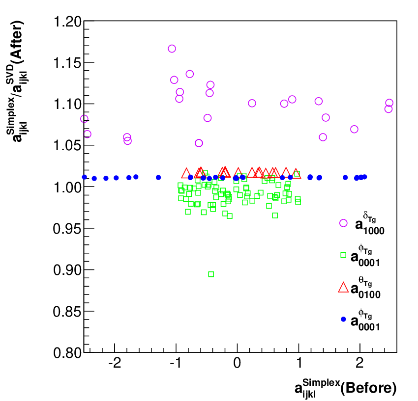
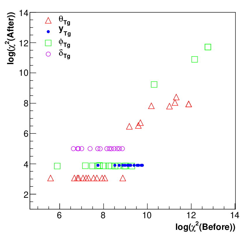
The results were considered to be stable if the defined by Eq. (4) converged to the same value for the majority of initial conditions. Small variations in were allowed: they are caused by small matrix elements which are irrelevant for , but have been set to non-zero values in order to additionally minimize in a particular minimization process. These matrix elements could be easily identified and excluded during the robustness checks because they are unstable and converge to a different value in each minimization. Ultimately only matrix elements that had the smallest fluctuations were kept for the matrix.
The SVD method was used next. To compute the matrix elements for , the linear set of Eqs. (6) first needs to be rewritten in the form used in Eq. (5):
where contains unknown matrix elements to be determined by the SVD, contains measured values of , and is filled with the products of detector variables accompanying the matrix elements in the polynomial expansion of Eq. (6) for each event.
The SVD analysis also began with matrix elements, but was not applied to one combined data set as in the simplex method in order to extract the most relevant ones. Rather, it was used on each set of data separately. From the comparison of the matrix elements obtained with different calibration data sets, only the elements fluctuating by less than were selected. Although this choice appears to be arbitrary, the results do not change much by modifying this criterion, for example, by including elements with as much as fluctuation. The final set of matrix elements contained only of the best entries. With these elements, the entire analysis was repeated in order to calculate their final values. The most relevant elements are listed in Table 2. The result of the calibration of is shown in Fig. 7.

5.2 Angular coordinates
For the calibration of the angular variables and , a set of quasi-elastic data on carbon and deuterium targets taken with the sieve-slit collimator was analyzed. The particles that pass through different holes can be well separated and localized at the detector plane.
By knowing the detector coordinates and the accurate position of the corresponding hole in the sieve, the target variables can be calculated. From the reaction point at the target (see Fig. 8), and can be calculated:
By using the values of the target variables, a set of linear equations has been written for all measured events, and matrix elements determined by using both numerical approaches. In the simplex method, matrix elements for and elements for were retained. Robustness checks for both angular variables were repeated to ensure that the global minimum had been reached.

The SVD analysis also started with matrix elements, which were ultimately reduced to for and for , again taking into account only those elements that fluctuated by less than . Figure 3 (right) shows the reconstructed sieve pattern. The majority of the holes are reconstructed, except those obscured by parts of the experimental apparatus due to specific geometric constraints during the experiment. In order to demonstrate the effect of gradually excluding redundant matrix elements, Fig. 9 shows the reconstructed top row of the sieve-slit collimator holes when the elements with up to , , and fluctuations are retained. There is virtually no difference in the reconstructed pattern when all elements exceeding the fluctuations are dropped, while errors start to appear when those fluctuating by less than are dropped.

The quality of the sieve-pattern reconstruction was examined by comparing the centers of the reconstructed holes with their true positions. Figure 10 shows that, with the exception of a few holes near the acceptance edges, these deviations are smaller than in the vertical, and smaller than in the horizontal direction. This is much less than the hole diameter, which is .

Once the sieve pattern was reconstructed, an absolute calibration had to be performed to correct for any BigBite misalignment and mispointing. For that purpose hydrogen and deuterium elastic data were used. By comparing the direction of the momentum transfer vector from the HRS to the calculated values of and , the zero-order matrix elements could be properly determined and the offsets corrected. In addition, the precise distance between the target and the sieve-slit collimator was obtained, which we were not able to measure precisely due to physical obstacles between the target and BigBite. From this analysis, the sieve slit was determined to be positioned away from the target.
5.3 Momentum
The matrix elements for the variable were obtained by using data from elastic scattering of electrons on hydrogen and deuterium for which the particle momentum in BigBite should be exactly the same as the momentum transfer given by the HRS. We assumed that depends only on and , while the dependencies involving and were neglected. Furthermore, the use of in-plane coordinates in the analysis for could result in an erroneous matrix due to the strong dependence inherent to elastic scattering (events strongly concentrated at one edge of the acceptance). Considering only and matrix elements, can be expressed as
| (26) |
In order to obtain the optics matrix applicable to all types of particles, energy losses for particle transport through the target enclosure and materials within the BigBite spectrometer were studied carefully. The energy losses were estimated by the Bethe-Bloch formula [29], but since the losses were significant, the formula had to be integrated over the complete particle track for each particle type and each initial momentum. The two largest contributions to the total momentum loss came from the target cell walls and from the air between the target and the detectors. (The latter losses could be alleviated by using a helium bag between the target and the detectors, but its benefits were considered to be smaller than the technical problems involved.) The resulting corrections that were taken into account in Eq. (26) are shown in Fig. 11 (left).


The elastic data available for calibration (momentum range approximately to ) covered only about half of the BigBite momentum acceptance. To calibrate the low-momentum region from to , we used protons from quasi-elastic scattering on by exploiting the information from the scintillator dE- and E-planes; the deposited particle energy in each plane was directly mapped to the particle momentum, based on known properties of the scintillator material. The punch-through point, corresponding to the particular momentum at which the particle has just enough energy to penetrate through the scintillators, served as a reference.
Beside the proton punch-through point, two other points with exactly known energy deposits in the dE- and E-planes were identified, as illustrated in Fig. 12. With the additional information from these points, a complete momentum calibration was possible. To compute the matrix elements, both numerical approaches described above were used. Since the available data were rather sparse, the search for the most stable matrix elements was not performed and a complete expansion to fifth order was considered in both techniques. Since only a two-variable dependency was assumed, a complete description was achieved by using only matrix elements.
The comparison of the most relevant matrix elements obtained from both numerical approaches is again shown in Table 2. Figure 12 (right) shows that the matrix is well under control. The reconstructed momentum agrees with the simulation of energy losses inside the scintillation planes for the complete momentum acceptance of BigBite, for both protons and deuterons. Figure 5 shows the missing-mass peak for the process. The resolution of the reconstructed neutron mass is approximately .


5.4 Resolution
The quality of the BigBite optics was also studied. The resolution of the vertex position was estimated from the difference between the reconstructed and the true position at the target by taking the width (sigma) of the obtained distribution. This part of the analysis was done by using -pass ( beam) quasi-elastic carbon data. The extracted values for the resolution of in different momentum bins can be parameterized as
where the particle momentum is in and the result is in meters. It is best at the upper limit of the accepted momentum range (about ) where it amounts to . The deterioration of the resolution at lower momenta is due to multiple scattering [29] in the air between the scattering chamber and the MWDCs.


The resolutions of and were estimated by comparing them to the corresponding angles as determined from the momentum transfer in elastic scattering on hydrogen and deuterium. The direction of is given by the electron kinematics and determined by the HRS spectrometer. The corresponding HRS resolutions have been studied in [30]. Based on these values, the resolution of the reconstructed was estimated to be and for the vertical and horizontal angles, respectively. These contributions were subtracted in quadrature from the calculated peak widths, yielding the final resolutions attributable to BigBite. The result for is shown in Fig. 13 (left). The strong momentum dependence of the resolution is again caused by multiple scattering in the target and the spectrometer. Different resolutions for deuterons and protons occur because the peak broadening in multiple scattering strongly depends on the particle mass (at a given momentum). As before, the biggest contributions come from the air. In a typical kinematics of the E05-102 experiment, the resolutions of and are and for protons, and approximately and for deuterons. (Due to multiple scattering, these resolutions are clearly much larger than the intrinsic MWDC resolutions mentioned in Section 2.)
The resolution of was also determined from elastic data by comparing the magnitude of to the momentum reconstructed by BigBite. The analysis was done separately for the hydrogen and deuterium data sets. Figure 13 (right) shows the relative momentum resolution as a function of momentum. The relative momentum resolution is approximately for protons, and for deuterons. Figure 5 (right) shows the absolute resolution of .
6 Summary
We have described the optics calibration of the BigBite spectrometer that was used to detect hadrons in the E05-102 experiment at Jefferson Lab. While the methods have been developed and applied to one spectrometer under very specific physical conditions, the same procedures can be applied to any spectrometer with a similar magnetic configuration and acceptance.
Two different approaches were considered: an analytical model that treats BigBite as an ideal dipole and a matrix formalism. The former approach results only in modest resolutions; still, resolutions of a few percent can be achieved by a suitable choice of parameters. The latter approach allows for a more precise calibration. Two numerical methods were used to determine the matrix elements, but the one based on singular value decomposition delivered better and more reliable results.
The vertex resolution for protons was found to be at along the whole target length. The resolution deteriorates significantly at lower momenta due to multiple scattering in the target, air, and detector material. The corresponding angular resolution is for the in-plane angle and for the out-of-plane angle . The angular resolution worsens at lower momenta due to multiple scattering, with the effect more pronounced for deuterons. The relative momentum resolution for protons (best case) has been estimated to be .
For deuterons (best case), we obtained the resolutions of (momentum), (), and ().
7 Acknowledgments
The Authors wish to thank Bogdan Wojtsekhowski for fruitful discussions and valuable advice on the manuscript.
This work was supported in part by the U.S. Department of Energy and the U. S. National Science Foundation. It is supported by DOE contract DE-AC05-06OR23177, under which Jefferson Science Associates, LLC, operates the Thomas Jefferson National Accelerator Facility. The UK collaborators acknowledge the funding by the UK Engineering and Physical Sciences Council and the UK Science and Technology Facilities Council.
References
- [1] D. J. J. Lange et al., Nucl. Instr. Meth. A 406 (1998) 182.
- [2] D. J. J. Lange et al., Nucl. Instr. Meth. A 412 (1998) 254.
- [3] J. Alcorn et al., Nucl. Instr. Meth. A 522 (2004) 294.
- [4] R. Subedi et al., Science 522 (2008) 1476.
- [5] R. Shneor et al., Phys. Rev. Lett. 99 (2007) 072501.
- [6] S. Riordan et al., Phys. Rev. Lett. 105 (2010) 262302.
- [7] R. Lindgren, B. E. Norum, J. R. M. Annand, V. Nelyubin (spokespersons), Precision measurements of electroproduction of near threshold: a test of chiral QCD dynamics, TJNAF Experiment E04-007.
- [8] X. Qian et al. (Hall A Collaboration), Phys. Rev. Lett. 107 (2011) 072003.
- [9] J. Huang et al. (Hall A Collaboration), Phys. Rev. Lett. 108 (2012) 052001.
- [10] S. Choi, X. Jiang, Z.-E. Meziani, B. Sawatzky (spokespersons), Precision measurements of the neutron : towards the electric and magnetic color polarizabilities, TJNAF Experiment E06-014.
- [11] S. Širca, S. Gilad, D. W. Higinbotham, W. Korsch, B. E. Norum (spokespersons), Measurement of and asymmetries in the quasi-elastic , TJNAF Experiment E05-102.
- [12] T. Averett, D. W. Higinbotham, V. A. Sulkosky (spokespersons), Measurements of the Target Single-Spin Asymmetry in the Quasi-Elastic Reaction, TJNAF Experiment E08-005.
- [13] E. Piasetzky, S. Gilad, B. Moffit, J. W. Watson, D. W. Higinbotham (spokespersons), Studying short-range correlations in nuclei at the repulsive core limit via the triple coincidence reaction, TJNAF Experiment E07-006.
- [14] Nilanga Liyanage, private communication.
- [15] R. W. Chan, MSc thesis, Construction and Characterization of Milti-wire Drift Chambers, University of Virginia, unpublished (2002).
- [16] R. Shneor, MSc thesis, High luminosity operation of large solid angle scintillator arrays in Jefferson Lab Hall A, Tel Aviv University, unpublished (2003). See also TJNAF reprint JLAB-PHY-03-219.
- [17] T. G. Walker, W. Happer, Rev. Mod. Phys. 69 (1997) 629.
- [18] E. Babcock, I. Nelson, S. Kadlecek, B. Driehuys, L. W. Anderson, F. W. Hersman, T. G. Walker, Phys. Rev. Lett. 91 (2003) 123002.
- [19] S. Penner, Rev. Sci. Instrum. 32 (1961) 150.
- [20] K. L. Brown, A first- and second-order matrix theory for the design of beam transport systems and charged particle spectrometers, SLAC Report 75, June 1982.
- [21] R. Shneor, PhD thesis, Investigation of proton-proton short-range correlations via the reaction, Tel Aviv University, unpublished (2008). See also TJNAF reprint JLAB-PHY-07-794.
- [22] W. Bertozzi et al., Nucl. Instrum. Meth. 162 (1979) 211.
- [23] N. Liyanage, Optics Calibration of the Hall A High Resolution Spectrometers using the C Optimizer, JLab Technical Note JLAB-TN-02-012 (2002).
- [24] J. A. Nelder, R. Mead, Comput. J. 7 (1965) 308.
- [25] W. H. Press et al., Numerical Recipes. The Art of Scientific Computing, Third Edition, Cambridge University Press, Cambridge, 2009.
- [26] G. Golub, W. Kahan, SIAM J. Numer. Anal. B 2 (1965) 205.
- [27] J. C. Lagarias, J. A. Reeds, M. H. Wright, P. E. Wright, SIAM J. Optim. 9 (1998) 112.
- [28] K. I. M. McKinnon, SIAM J. Optim. 9 (1998) 148.
- [29] W. R. Leo, Techniques for Nuclear and Particle Physics Experiments, Springer-Verlag, Heidelberg, 1987.
- [30] G. Jin, PhD thesis, Extraction of at from Measurements of , University of Virginia, unpublished (2011).